Consistency of Histories of Neutrino Oscillation in the Presence of Normal Matter and Continuous Non-Selective Measurement

Abstract

Two-flavor neutrino oscillation is analyzed using the consistent histories approach. We identify the properties of neutrinos and the oscillation conditions, such as the presence of matter or the impact of measurement, that ensure the consistency of three-time neutrino histories. The connection between the consistency of these histories and the well-known CP violation explored in this study serves as a specific example.

1. Introduction

Neutrinos, often hypothesized as key to understanding the Universe and its origins, are studied across various disciplines. At the heart of this research are the fascinating dynamical properties of neutrino oscillations [1,2,3], which, while naturally investigated within the realm of particle physics [4], have also garnered interest from the perspectives of decoherence [1,5,6,7,8,9,10] and quantum information processing [2,11,12,13,14,15,16,17]. Sophisticated experiments [18] have illuminated some of these properties, yet many fundamental questions about the time evolution of neutrinos [4,19] and their oscillations remain unresolved.

As neutrinos hardly interact with anything, they have legitimately become a template for examples and studies concerning systems resistant to measurements, and open up further avenues of research. In the absence of a measurement scheme of the mass of a neutrino, one can adopt the typical terminology associated with quantum measurement [20,21], and study neutrino oscillations in a model that mimics Continuous Non-Selective measurement by environment [17].

Alternatively, one can move beyond the orthodox interpretations of measurement and employ the Consistent (or Decoherent) Histories Formalism to extract information about systems where direct measurements are unavailable due to fundamental or technical limitations [22,23,24,25,26]. A quantum history of a physical system consists of a sequence of quantum events at successive times, where a quantum event at a given time represents any quantum property of the system in question [22]. For instance, a neutrino being in a specific mass state constitutes such an event. If a family of these histories is shown to be consistent, probabilities can be assigned to the occurrence of these events. Conversely, one can investigate the properties or parameters necessary to render a family of histories consistent.

In this paper, following a brief review of neutrino oscillations, continuous non-selective measurement, and the consistent history approach, we analyze the impact on the consistency of a family of histories for a neutrino oscillating in the presence of matter. Specifically, we consider the role of decoherence induced by a mechanism that mimics a continuous non-selective measurement [20] of an “observable” analogous to a hypothetical measurement of neutrino mass.

We consider a simplified two-flavor model of neutrino oscillations, focusing on electron–muon oscillations [1,4,19,27,28]. Despite its simplicity, this model provides valuable insights into the dynamics of neutrino oscillations. Additionally, we examine three time histories of the two-flavor neutrino evolution. These histories represent the shortest non-trivial sequences that cannot be analyzed using the standard Born rule. Each three-time history is so named because it consists of three “events”. In our analysis, the first and third events correspond to the neutrino being in a flavor state, while the second event places the neutrino in a mass state [29].

The presence of matter is crucial for achieving the consistency of such three-time families of histories in neutrino oscillations [29], particularly when there is a scattering-like interaction between neutrinos and ordinary matter. In this paper, we treat the system as an open quantum system, where a specific type of decoherence arises from a hypothetical non-selective measurement-like quantum-classical environment, which affects the oscillations [17]. While potential CP violation from a hypothetical non-vanishing Majorana phase does not influence the consistency of the histories considered [29], our focus is on investigating how the back-effect from continuous non-selective measurements impacts the consistency of these histories. Additionally, we explore whether this back-effect introduces a dependence on the consistency of the Majorana phase.

2. Qubit Approximation of Neutrinos

The qubit approximation utilizes a two-level system, where a neutrino can exist in two flavor states $v_e,v_{\mu }$, which do not directly correspond to the two mass states $v_1,v_2$, allowing for simpler mixing parameters and often enabling analytical solutions. The flavor states are expressed as $\mid v_e⟩=cos\theta \mid 1⟩+e^{i\varphi }sin\theta \mid 2⟩$ and $\mid v_{\mu }⟩=-sin\theta \mid 1⟩+e^{i\varphi }cos\theta \mid 2⟩$, where $\theta ={\theta }_{12}$ is the mixing angle. The phase $\varphi$ represents the CP-violating Majorana phase, which vanishes under the $U\left(1\right)$ global transformation in the Dirac phase but remains non-zero in the Majorana case [4].

The vacuum Hamiltonian for a two-level relativistic neutrino [4] is given by

$$\begin{array}{ccc}\hfill H_0& =& \left(\begin{array}{cc}E-{\displaystyle \frac{\Delta m_{21}^2}{4E}}& 0\\ 0& E+{\displaystyle \frac{\Delta m_{21}^2}{4E}}\end{array}\right)\hfill \end{array}$$

(1)

where $\Delta m_{21}^2=m_2^2-m_1^2$ is the mass-squared difference in the normal hierarchy case, and E is the energy of the massless neutrino. The effective Hamiltonian for a neutrino propagating in normal matter, known as the Wolfenstein effective Hamiltonian [1,4], is given by the following:

$$\begin{array}{ccc}\hfill H_F& =& H_0+{\displaystyle \frac{V_0}{2}}\left(\begin{array}{cc}1+cos2\theta & e^{-i\varphi }sin2\theta \\ e^{i\varphi }sin2\theta & 1-cos2\theta \end{array}\right)\hfill \end{array}$$

(2)

where $N_e$ is the electron density, $G_F$ is the Fermi constant, and $V_0=\sqrt{2}{G}_F{N}_e$ is the effective interaction potential due to the oscillation of the neutrino in the presence of normal matter, arising from coherent forward scattering on electrons via charged current interactions. The neutral current interaction does not contribute effectively to the Hamiltonian as per the Standard Model [4].

3. Continuous Non-Selective Measurement

Quantum measurements are fundamentally different from the classical concept of measurement. Real experiments attempting to measure physical quantities can rarely be fully described by the von Neumann scheme [20,21,30], in which the system being measured and the apparatus performing the measurement interact to produce what we refer to as a measurement.

For quantum systems, measurement is not direct and can be thought of as a two-step process. The system being measured interacts with another system that acts as a measurement probe. This probe, as a system, has properties that can be read by a classical apparatus. Thus, an observable A of the quantum system couples to the probe’s position Q, resulting in an interaction between the system and the probe. Next, the probe’s momentum P, canonically conjugated to Q, is projectively measured. The first part of this process can be viewed as the act of making the measurement, while the second part represents the reading of the measurement made [20,21,30].

A continuous measurement involves the continual extraction of information from a system, whereas a non-selective measurement is one where the result is ignored or not read [20]. Therefore, we treat the interaction with the environment as a neutrino propagates in the presence of normal matter as a continuous measurement-like interaction, where the result is not read [17]. The first part of the measurement is described by the system-probe total Hamiltonian:

$$\begin{array}{c}\hfill H_{sys+probe}=H_{sys}+H_{probe}+g\left(t\right)H_{int}\end{array}$$

(3)

where $g\left(t\right)$ is the strength of the coupling. The observable A of a quantum system couples with the probe’s position Q to give the interaction term $H_{int}=A\otimes Q.$

Assuming a non-selective measurement over a time interval divided into intervals of length q, the dynamics of the system, after being reduced with respect to the probe, are no longer unitary; however, they form a completely positive quantum map. For a set of measurement operators $E_x$, where ${\sum }_x{E^{†}}_x{E}_x=\mathbb{I}$, the non-selective measurement of a system in state $\rho$ is the transformation $\rho \to E_x\rho {E^{†}}_x,$ which is an example of a completely positive map [31].

The evolution of the state due to such a measurement on each time interval of length q is given by the following:

$$\begin{array}{c}\hfill \rho (t+q)=\int dp{E}_p\rho \left(t\right)E^{†}p\end{array}$$

(4)

with $E_p=e^{iqHsys}⟨p\mid e^{-iq{H}_{int}}\mid {\varphi }_q⟩.$ Here, $\mid p⟩\in H_{probe}$ is an eigenstate of P, the probe momentum, and $\mid {\varphi }_q⟩\in H_{probe}$ is the state of the probe before the measurement. Expanding Equation (4) to the second order in q for a finite measurement duration leads to a quantum master equation:

$$\begin{array}{c}\hfill {\displaystyle \frac{d}{dt}}\rho \left(t\right)=-i[H_{sys},\rho \left(t\right)]-{\displaystyle \frac{\sigma }{2}}[A,[A,\rho \left(t\right)]]\end{array}$$

(5)

where the first term represents the extraction of information due to the measurement process, and the second term represents the back-action on the state of the system due to the measurement [31,32].

The parameter $\sigma$ describes the back-action of the measurement. For an integrated coupling strength proportional to the length of the time interval $q\sim {\int }_0^{t}g\left(s\right)ds$, $\sigma$ is given by the following:

$$\begin{array}{c}\hfill {\sigma }^2=\underset{q\to 0}{lim}q⟨{\varphi }_q\mid Q^2\mid {\varphi }_q⟩\end{array}$$

(6)

where the limit describes the transition from a step-like to a truly continuous measurement.

We consider a continuous non-selective measurement of a neutrino to be described by the master Equation (5), where

$$\begin{array}{c}\hfill H_{sys}=H_F\end{array}$$

(7)

and the “observable” that is hypothetically measured corresponds to a mass state measurement, diagonal in the mass state basis,

$$\begin{array}{c}\hfill M=\sum _{x=1,2}{a}_x{\Pi }_x,;\mathrm{where};{\Pi }_x=\mid x⟩⟨x\mid ,;x=1,2\end{array}$$

(8)

where $a_1=-a_2$ [17].

Selective measurements of neutrinos are rare and challenging, but this model presents a close to non-selective case, which increases the probability of transition from the electron flavor to the muon flavor, and even more so for CP-violating systems [17].

4. Consistent Histories Formalism for Qubit Approximation of Neutrino Oscillation

The Consistent Histories approach treats measurement beyond the traditional Copenhagen interpretation of Quantum Mechanics. It defines a quantum event as any quantum property of the system at a particular time, and a quantum history as a sequence of such quantum events at successive times [22], making each history a compound quantum event that represents a specific time evolution of the system. The time evolution of the system is treated as a stochastic process, meaning that the past or future states of the system are not determined by the present state.

Each quantum event is mathematically represented as a projection operator P corresponding to the quantum property that defines the event. Thus, a quantum history, analogous to a stochastic process, of length n is a sequence of projectors $P_i$, with one projector for each time $t_i$, where $i=0,\dots ,(n-1)$. Since the process is akin to a stochastic process, the events come from a well-defined event algebra, which is obtained by considering quantum events that are mutually exclusive to each other, with the projectors representing these events summing up to the identity.

$$\begin{array}{cc}\hfill P^j{P}^k& ={\delta }_{jk}{P}^k,\sum _j{P}^j=I\hfill \end{array}$$

(9)

In other words, one does not consider just a single history, but a complete family of histories [22,33]. Thus, these families of histories are composed of projective decompositions of the identity, $PDI=P^k$, which is referred to as a framework, and must originate from a single framework in order to include only compatible properties, as per the single framework rule [22,33,34,35].

At each time instant $t_i$, all the quantum properties of the system correspond to elements of a $PDI\left(t_i\right)$, with each projector mapping quantum states onto subspaces of the instantaneous Hilbert Space $\mathcal{H}\left(t_i\right)$. The space for a history is mathematically the tensor product of the instantaneous Hilbert Spaces:

$$\begin{array}{cc}\hfill \breve{\mathcal{H}}& =\underset{i=0}{\overset{n}{⨀}}\mathcal{H}\left(t_i\right)\hfill \end{array}$$

(10)

where ⊙ represents the temporal composite (multi-time), in contrast to ⊗, which is used for spatial composites (multi-partite) [22].

Each history $M^k$ can then be expressed as

$$\begin{array}{cc}\hfill M^k& =\underset{i=0}{\overset{n}{⨀}}{P}^{(i,k)}\hfill \end{array}$$

(11)

where $P^{(i,k)}\in PDI\left(t_i\right)$. The consistency condition involves assigning probabilities, or weights, to non-commuting quantum properties only if there is no interference between pairs of histories that should be decoherent. Weights for histories are derived by extending the Born rule to multi-time histories [22,23,33,34,35], and are computed as

$$\begin{array}{cc}\hfill W\left(M^k\right)& =⟨K\left(M^k\right),K\left(M^k\right)⟩=\mathrm{T}\mathrm{r}\left[K^{†}\left(M^k\right)K\left(M^k\right)\right]\hfill \end{array}$$

(12)

where for a time evolution operator $T(t_i,t_j),$$K\left(M^k\right)$ is called the history’s chain operator [22].

$$\begin{array}{cc}\hfill K\left(M^k\right)& =P^{(n,k)}\prod _{i=0}^{n-1}T(t_{i+1},t_i)P^{(i,k)}=P_{n}T(t_n,t_{n_1})P_{n-1}\cdots P_{1}T(t_1,t_0)P_0\hfill \end{array}$$

(13)

The decoherence of histories comes from the consistency condition [22,23,33,34,35], which is formulated as follows:

$$\begin{array}{c}\hfill ⟨K\left(M^k\right),K\left(M^s\right)⟩=0,forallk\ne s\end{array}$$

(14)

There is a qualitative distinction between histories with zero weight (vanishing probability) and inconsistent families of histories [22]. Histories M such that $K\left(M\right)=0$ represent events that do not occur and are referred to as dynamically impossible histories. Inconsistent families of histories have no meaning within the consistent histories framework, and no weight or probability can be assigned to such families through time evolution governed by the laws of quantum dynamics [22,35]. It is also possible to write families of histories that are inherently inconsistent, regardless of the time evolution governing the system. However, of greater interest are families of histories that are largely inconsistent unless the dynamics that evolve the system over time adopt certain parameters, where solving the consistency condition is equivalent to identifying those parameters.

One such example is the one explored in [29], a family of three-time histories which is also the one we study further in this paper.

$$\begin{array}{cc}\hfill M^0& :\left[v_{\mu }\right]\odot \left[I\right]\odot \left[I\right]\hfill \\ \hfill M^1& :\left[v_e\right]\odot \left[1\right]\odot \left[v_{\mu }\right]\hfill \\ \hfill M^2& :\left[v_e\right]\odot \left[1\right]\odot \left[v_e\right]\hfill \\ \hfill M^3& :\left[v_e\right]\odot \left[2\right]\odot \left[v_{\mu }\right]\hfill \\ \hfill M^4& :\left[v_e\right]\odot \left[2\right]\odot \left[v_e\right]\hfill \end{array}$$

(15)

where $\left[x\right]=|x⟩⟨x|,x={\nu }_{e,\mu },1,2$. All histories begin with the neutrino in the electron flavor state, except for $M^0$, which is required to obtain the PDI. At the second time instance, the histories place the neutrino in a mass state, followed by a return to a flavor state at the third time instance. The history $M^0$ can be expanded into four similar histories, where the initial state is a muon flavor neutrino, evolving to a mass state at the second time instance, and returning to a flavor state at the third, much like the histories for the electron neutrino, with the same results [29].

Utilizing Equation (13), the chain operators for the family of histories are obtained as follows:

$$\begin{array}{cc}\hfill K\left(M^0\right)& =T_2{T}_1\mid v_{\mu }⟩⟨v_{\mu }\mid \hfill \\ \hfill K\left(M^1\right)& =⟨v_{\mu }\mid T_2\mid 1⟩⟨1\mid T_1\mid v_e⟩.\mid v_{\mu }⟩⟨v_e\mid \hfill \\ \hfill K\left(M^2\right)& =⟨v_e\mid T_2\mid 1⟩⟨1\mid T_1\mid v_e⟩.\mid v_e⟩⟨v_e\mid \hfill \\ \hfill K\left(M^3\right)& =⟨v_{\mu }\mid T_2\mid 2⟩⟨2\mid T_1\mid v_e⟩.\mid v_{\mu }⟩⟨v_e\mid \hfill \\ \hfill K\left(M^4\right)& =⟨v_e\mid T_2\mid 2⟩⟨2\mid T_1\mid v_e⟩.\mid v_e⟩⟨v_e\mid \hfill \end{array}$$

(16)

where $T_1=exp\left[i(t_0-t_1)H\right]$ and $T_2=exp\left[i(t_1-t_2)H\right]$ represent the time evolution operators for the first and second intervals of the three-time histories. By applying the consistent histories Equation (14) to each pair of histories in the family, all histories are mutually exclusive to each other, except for $M^1$ versus $M^3$, and $M^2$ versus $M^4$ [29], which are given as follows:

$$\begin{array}{cc}\hfill ⟨K\left(M^1\right)\mid K\left(M^3\right)⟩& =⟨1\mid T_2^{†}\mid v_{\mu }⟩⟨v_e\mid T_1^{†}\mid 1⟩⟨v_{\mu }\mid T_2\mid 2⟩⟨2\mid T_1\mid v_e⟩\hfill \\ \hfill ⟨K\left(M^2\right)\mid K\left(M^4\right)⟩& =⟨1\mid T_2^{†}\mid v_e⟩⟨v_e\mid T_1^{†}\mid 1⟩⟨v_e\mid T_2\mid 2⟩⟨2\mid T_1\mid v_e⟩\hfill \end{array}$$

(17)

The case in which there is no back-effect from the environment and the time evolution operators T are derived from $H=H_F$ as given in Equation (2) was solved in [29] by determining the parameters that make

$$\begin{array}{cc}\hfill ⟨K\left(M^1\right)\mid K\left(M^3\right)⟩& \equiv 0\hfill \\ \hfill ⟨K\left(M^2\right)\mid K\left(M^4\right)⟩& \equiv 0\hfill \end{array}$$

(18)

and render the family of histories consistent. For these dynamics, the family of histories is inconsistent in a vacuum, but in the presence of normal matter, where $V_0={\displaystyle \frac{\Delta m_{21}^2}{2E}}$ and the parameter $D={\displaystyle \frac{n\pi }{t}}$, the family becomes consistent. Here, D is defined as the difference between the eigenvalues of $H_F$, specifically $D={\lambda }_1-{\lambda }_2$ [29].

In this paper, we consider a two-flavor neutrino oscillating in the presence of normal matter, where the environment simulates a continuous non-selective measurement of the observable M from Equation (8). This interaction introduces the back-action $\sigma$ in the quantum master Equation (5), with $H_{sys}=H_F$, allowing us to derive the time evolution operator T for this process. We then solve Equation (18) to identify the dynamical parameters that make the family of histories (15) consistent under these dynamics. We demonstrate that the additional effect of the environment simulating a continuous non-selective measurement of the “mass observable” expands the range of parameter values that lead to consistency.

5. Method

In the mass basis, the qubit neutrino can be expressed as

$$\begin{array}{ccc}\hfill H_{sys}& =& \left(\begin{array}{cc}A& e^{-i\varphi }C\\ e^{i\varphi }C& B\end{array}\right)\hfill \end{array}$$

(19)

where

$$\begin{array}{cc}\hfill A& =E-{\displaystyle \frac{\Delta m_{21}^2}{4E}}+{\displaystyle \frac{V_0}{2}}(1+cos2\theta )\hfill \\ \hfill B& =E+{\displaystyle \frac{\Delta m_{21}^2}{4E}}+{\displaystyle \frac{V_0}{2}}(1-cos2\theta )\hfill \\ \hfill C& ={\displaystyle \frac{V_0}{2}}sin2\theta \hfill \end{array}$$

(20)

$D,$ which is ${\lambda }_1-{\lambda }_2,$${\lambda }_{1,2}$ being eigenvalues of $H_{sys},$ can then be expressed as

$$D=\sqrt{{(A-B)}^2+4C^2}.$$

The mass observable being measured can be expressed as follows:

$$\begin{array}{cc}\hfill M& =\mid 1⟩⟨1\mid -\mid 2⟩⟨2\mid =\left(\begin{array}{cc}1& 0\\ 0& -1\end{array}\right)\hfill \end{array}$$

(21)

To solve the master equation, we rewrite it in the form $\dot{\rho }=\widehat{\mathcal{L}}\rho$, where $\widehat{\mathcal{L}}$ is the Liouvillian superoperator. We then parameterize the system in Bloch space, resulting in the following expression for $\mathcal{L}$:

$$\begin{array}{ccc}\hfill \mathcal{L}& =& \left(\begin{array}{ccc}-2{\sigma }^2& B-A& 2Csin\varphi \\ A-B& -2{\sigma }^2& -2Ccos\varphi \\ -2Csin\varphi & 2Ccos\varphi & 0\end{array}\right)\hfill \end{array}$$

(22)

The solution to Equation (5) then comes from solving the equation below:

$$\begin{array}{c}\hfill ⟨\dot{\sigma }⟩=\mathcal{L}⟨\sigma ⟩\end{array}$$

(23)

However, as we do not need to compute the states of the system, but just the time evolution dynamics to use for checking consistency, we do not need a full solution to the master equation, but just compute $e^{\mathcal{L}t}$ to obtain the time development operator $T=e^{\mathcal{L}t}.$ Having $T,$ we substitute it to Equation (17) and solve for Equation (18).

Computing $e^{\mathcal{L}t}$ requires determining the eigenvalues of $\mathcal{L}$. While the matrix $H_F$ could be solved analytically, the introduction of the back-effect from the continuous non-selective measurement necessitates solving for $\mathcal{L}$ computationally. All computations for this paper were performed using SageMath (https://www.sagemath.org/). The characteristic equation for the eigenvalues of $\mathcal{L}$ is given by the following:

$$\begin{array}{c}\hfill {\lambda }^3+4{\sigma }^2{\lambda }^2+(D^2+4{\sigma }^4)\lambda +8C^2{\sigma }^2=0\end{array}$$

(24)

The eigenvalues are thus the solutions to Equation (24), computed through the SageMath eigenvalue function, which turns out to be

$$\begin{array}{cc}\hfill {\lambda }_1& ={\displaystyle \frac{1}{3}}[y-X-4{\sigma }^2]\hfill \\ \hfill {\lambda }_2& ={\displaystyle \frac{1}{6}}[(X-y-8{\sigma }^2)-i\sqrt{3}(X+y)]\hfill \\ \hfill {\lambda }_3& ={\displaystyle \frac{1}{6}}[(X-y-8{\sigma }^2)+i\sqrt{3}(X+y)]\hfill \end{array}$$

(25)

where we define

$$\begin{array}{cc}\hfill y^3& =8{\sigma }^6+18{\sigma }^2[{(A-B)}^2-2C^2]+\sqrt{432{\sigma }^8{(A-B)}^2+27D^6+216{\sigma }^4[{(A-B)}^4-10{(A-B)}^2{C}^2-2C^4]}\hfill \\ \hfill X& ={\displaystyle \frac{3D^2-4{\sigma }^4}{y}}\hfill \end{array}$$

(26)

As per the Cayleigh–Hamilton Theorem, each matrix satisfies its own characteristic equation, therefore,

$$\begin{array}{c}\hfill \Delta \left(\mathcal{L}\right)={\mathcal{L}}^3+{\sigma }^2{\mathcal{L}}^2+(D^2+4{\sigma }^4)\mathcal{L}+8C^2{\sigma }^2=\left[0\right]\end{array}$$

(27)

Any analytic function $f\left(A\right)$ of a matrix A can be written as $f\left(A\right)={\sum }_{k=0}^{\infty }{\alpha }_k{A}^k,$ which can be written as a polynomial as $f\left(s\right)={\sum }_{k=0}^{\infty }{\alpha }_k{s}^k.$ Per Remainder Factor Theorem, $f\left(s\right)=\Delta \left(s\right)Q\left(s\right)+R\left(s\right),$ where $\Delta \left(s\right),$$Q\left(s\right),$ and $R\left(s\right)$ are the divisor, quotient, and remainder, respectively. However, for $s=\lambda ,$ we obtain

$$\begin{array}{c}\hfill f\left(\lambda \right)=\Delta \left(\lambda \right)Q\left(\lambda \right)+R\left(\lambda \right)=R\left(\lambda \right)=\sum _{k=0}^{n-1}{\alpha }_k{\lambda }^k\end{array}$$

(28)

Similarly, $f\left(A\right)=\Delta \left(A\right)Q\left(A\right)+R\left(A\right),$ for a matrix $A.$ By the Cayleigh–Hamilton Theorem, $\Delta \left(A\right)=0.$ Therefore,

$$\begin{array}{c}\hfill f\left(A\right)=\sum _{k=0}^{n-1}{\alpha }_k{A}^k\end{array}$$

(29)

such that ${\alpha }_k$ satisfy $f\left({\lambda }_i\right)={\sum }_{k=0}^{n-1}{\alpha }_k{\lambda }_i^k.$ Therefore, $\mathcal{L}$ being a $3\times 3$ matrix, and $exponential$ being an analytic function, by Equation (28),

$$\begin{array}{c}\hfill e^{\mathcal{L}t}={\alpha }_0\mathbb{I}+{\alpha }_1\mathcal{L}+{\alpha }_2{\mathcal{L}}^2\end{array}$$

(30)

where ${\alpha }_0,$${\alpha }_1,$ and ${\alpha }_2$ satisfy the system of equations

$$\begin{array}{c}\hfill e^{{\lambda }_{i}t}=\sum _{k=0}^2{\alpha }_k{\lambda }_i^k\end{array}$$

(31)

Additionally, $e^{\mathcal{L}t}$ will be used to solve Equation (18), with the full forms of the consistency condition provided in Equation (17). There are two intervals between the three events in each history: $t_1$ corresponds to the time interval between the initial pure flavor state and the pure mass state, and $t_2$ represents the time interval between the pure mass state and the pure flavor state. To obtain a solution, we consider only one time t. The choice of $t_1$ or $t_2$ to achieve consistency influences the probabilities of the histories but does not affect the solution itself. Thus, the solution to Equation (18), which ensures the consistency of this family of histories (15), can be expressed as follows:

$$\begin{array}{c}\hfill T\left[v_e\right]=\left[1\right]or{T}^{†}\left[1\right]=\left[v_{\mu }\right]\end{array}$$

(32)

Each of the two consistency equations in (32) provides a different set of values for the parameters ${\alpha }_0$, ${\alpha }_1$, and ${\alpha }_2$. However, these parameters must also satisfy the system of equations derived from $e^{{\lambda }_{i}t}={\sum }_{k=0}^2{\alpha }_k{\lambda }_i^k$. We define

$$\begin{array}{c}\hfill z={\displaystyle \frac{\sqrt{3}(X+y)[3{\alpha }_1+(X-y-8{\sigma }^2){\alpha }_2]}{18{\alpha }_0+3(X-y-8{\sigma }^2){\alpha }_1-(X^2+4Xy+y^2+8{\sigma }^2(X-y)-32{\sigma }^4){\alpha }_2}}\end{array}$$

(33)

Thus, solving the set of equations parameters ${\alpha }_0,$${\alpha }_1,$ and ${\alpha }_2$ can be simplified into one multi-variate equation below:

$$\begin{array}{c}\hfill f(V_0,{\sigma }^2)={\displaystyle \frac{t}{3}}\left[y-X-4{\sigma }^2\right]-ln\left[{\displaystyle \frac{1}{9}}(9{\alpha }_0+3(y-X-4{\sigma }^2){\alpha }_1+{(y-X-4{\sigma }^2)}^2{\alpha }_2)\right]=0\end{array}$$

(34)

such that ${\displaystyle \frac{\sqrt{3}}{6}}(X+y)t=ta{n}^{-1}\left(z\right)\ne 0.$

For $T\left[v_e\right]=\left[1\right],$

$$\begin{array}{cc}\hfill {\alpha }_0& ={\displaystyle \frac{8{\sigma }^4(Ccos2\theta -(A-B)sin2\theta )sin2\theta }{8{\sigma }^4(Ccos2\theta -(A-B)sin2\theta )\left(sin2\theta cos2\theta \right)-((A-B)cos2\theta +2Csin2\theta ){(2Ccos2\theta -(A-B\left)sin2\theta \right)}^2}}\hfill \\ \hfill {\alpha }_1& ={\displaystyle \frac{4{\sigma }^2(Ccos2\theta -(A-B)sin2\theta )sin2\theta }{8{\sigma }^4(Ccos2\theta -(A-B)sin2\theta )\left(sin2\theta cos2\theta \right)-((A-B)cos2\theta +2Csin2\theta ){(2Ccos2\theta -(A-B\left)sin2\theta \right)}^2}}\hfill \\ \hfill {\alpha }_2& ={\displaystyle \frac{(2Ccos2\theta -(A-B\left)sin2\theta \right)sin2\theta }{8{\sigma }^4(Ccos2\theta -(A-B)sin2\theta )\left(sin2\theta cos2\theta \right)-((A-B)cos2\theta +2Csin2\theta ){(2Ccos2\theta -(A-B\left)sin2\theta \right)}^2}}\hfill \end{array}$$

(35)

For $T^{†}\left[1\right]=\left[v_{\mu }\right],$

$$\begin{array}{cc}\hfill {\alpha }_0& =-{\displaystyle \frac{(A-B)cos2\theta +2Csin2\theta }{(A-B)}}\hfill \\ \hfill {\alpha }_1& =-{\displaystyle \frac{{\sigma }^{2}sin2\theta }{(A-B)C}}\hfill \\ \hfill {\alpha }_2& =-{\displaystyle \frac{sin2\theta }{2(A-B)C}}\hfill \end{array}$$

(36)

We further parameterize and scale the time t in units of E as $V_0=\acute{V}{\displaystyle \frac{\Delta m_{21}^2}{2E}}$, ${\sigma }^2={\acute{\sigma }}^2{\displaystyle \frac{\Delta m_{21}^2}{2E}}$, and $t=\acute{t}{\displaystyle \frac{2E}{\Delta m_{21}^2}}$, then solve for $f(\acute{V},{\acute{\sigma }}^2)=0$. This renders $\acute{V}$ and ${\acute{\sigma }}^2$ to be dimensionless, and ${\displaystyle \frac{\sqrt{3}}{6}}(X+y)\acute{t}$ is in radians. Furthermore, this also factors out ${\displaystyle \frac{\Delta m_{21}^2}{2E}}$ from Equation (34), making the computations more precise. We also use known experimental estimates for solar neutrinos: $\theta ={{33.68}^{\circ }}_{-0.70}^{+0.73}$ [36] for the computation. For each case, we substitute $\theta ,$ and the corresponding parameters ${\alpha }_0,{\alpha }_1,$ and ${\alpha }_2,$ and plot the function f using the SageMath plot function to search for solutions for $f=0.$

6. Results

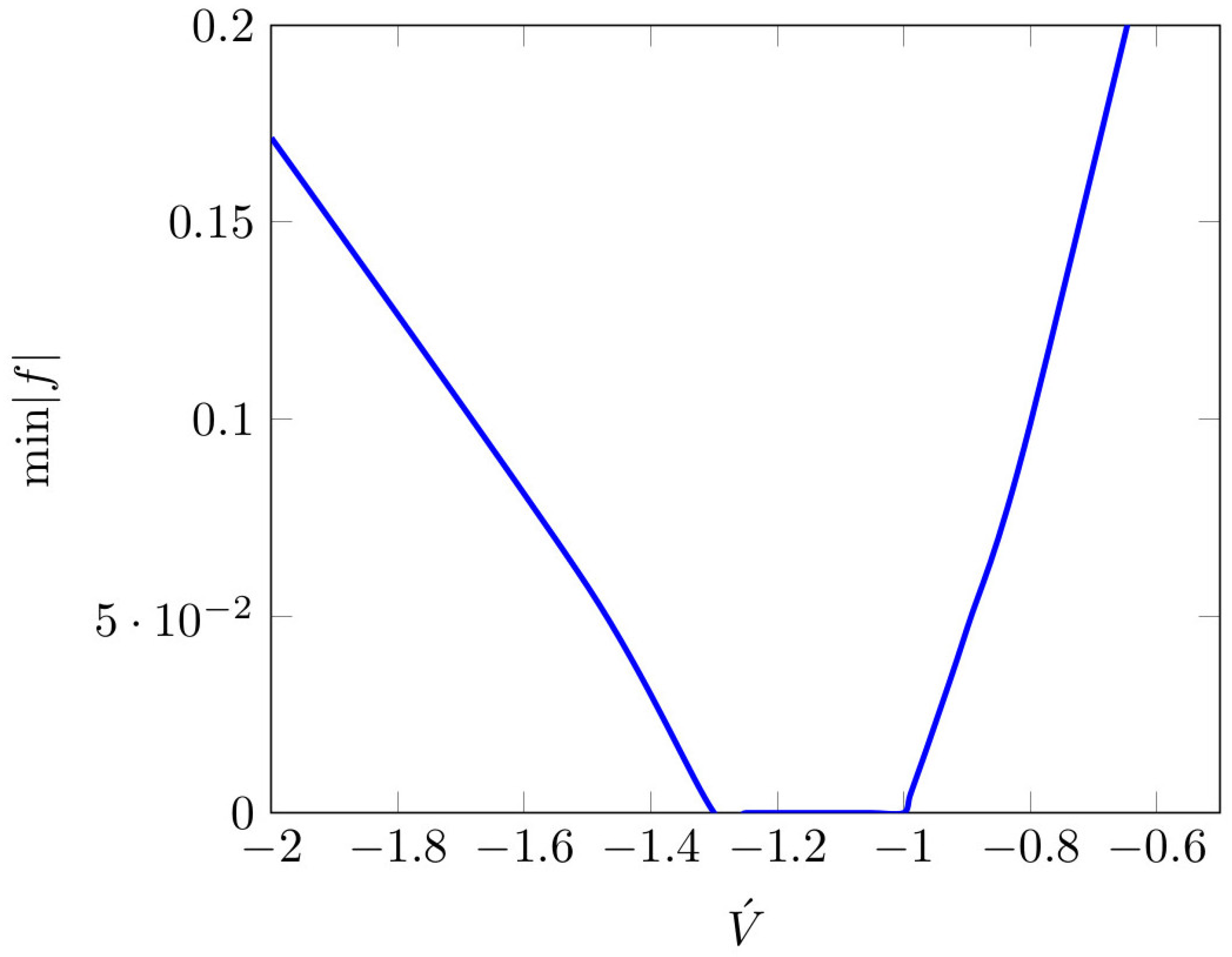
Initially, we obtained the range of values of $\acute{V}$ such that $f(\acute{V},{\acute{\sigma }}^2)=0,$ for ${\acute{\sigma }}^2\ge 0.$ Once the range of values of $\acute{V}$ has been computed, we look for a corresponding set of values of ${\acute{\sigma }}^2$ that led to $f=0$. Figure 1 shows the minimum of the absolute value of f for values of $\acute{V}$ for case (i), where $T\left[v_e\right]=\left[1\right]$. Figure 2 shows the minimum of the absolute value of f for values of $\acute{V}$ for case (ii), where $T^{†}\left[1\right]=\left[v_{\mu }\right]$. Both figures have been zoomed into the range where $min\left|f\right|$ nears 0 only.

Figure 1. Set of values of $\acute{V}$ and $min\left|f\right|$ for $T\left[v_e\right]=\left[1\right].$ The figure plots the minimum of the absolute value of $f,$ vertical axis, for ${\acute{\sigma }}^2\ge 0,$ against each value of $\acute{V},$ horizontal axis. The figure has been zoomed in to show the range where $min\left|f\right|$ nears 0 only.

Figure 2. Set of values of $\acute{V}$ and $min\left|f\right|$ for $T^{†}\left[1\right]=\left[v_{\mu }\right].$ The figure plots the minimum of the absolute value of $f,$ vertical axis, for ${\acute{\sigma }}^2\ge 0,$ against each value of $\acute{V},$ horizontal axis. The figure has been zoomed in to show the range where $min\left|f\right|$ nears 0 only.

For $T\left[v_e\right]=\left[1\right],$ Figure 1 shows that Equation (34) is satisfied for negative values of $\acute{V},$≈$-1.3\le \acute{V}\le -1,$ that is ≈$-1.3{\displaystyle \frac{\Delta m_{21}^2}{2E}}\le V_0\le -1{\displaystyle \frac{\Delta m_{21}^2}{2E}}$. This we reject as non-physical. For $T^{†}\left[1\right]=\left[v_{\mu }\right],$ the solution lies with the range $1\le \acute{V}\le \approx 1.24,$ that is ${\displaystyle \frac{\Delta m_{21}^2}{2E}}\le V_0\le \approx 1.24{\displaystyle \frac{\Delta m_{21}^2}{2E}}$.

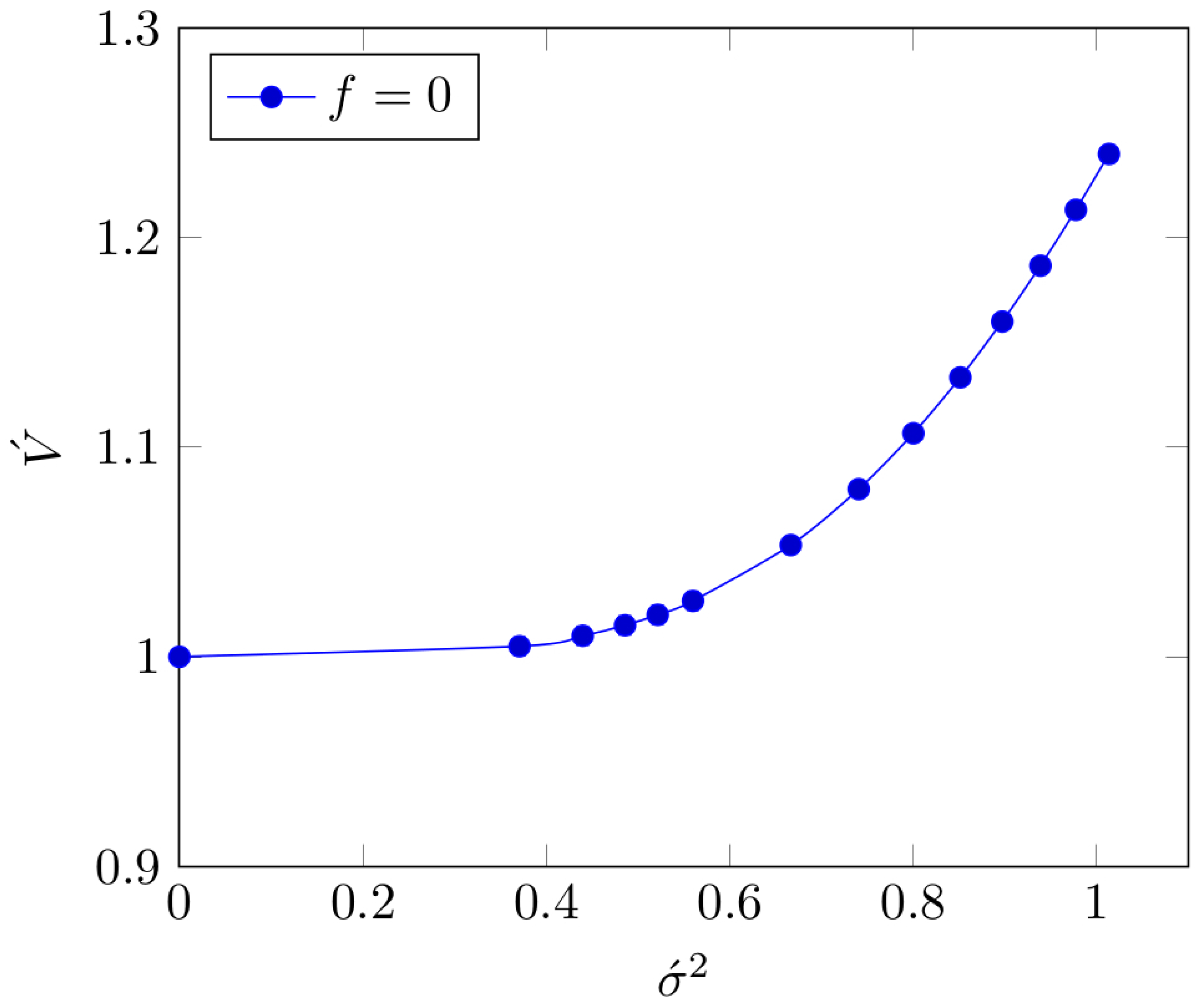
We proceed further to search for consistency in the second case only, that is $T^{†}\left[1\right]=\left[v_{\mu }\right].$ Figure 3 displays the set of values for $\acute{V}$ and ${\acute{\sigma }}^2$ where $f(V_0,{\sigma }^2)=0$ for $T^{†}\left[1\right]=\left[v_{\mu }\right]$. The figure is followed by Table 1 which lists the values used for plotting Figure 3, along with the corresponding values for ${\displaystyle \frac{\sqrt{3}}{6}}(X+y)\acute{t}$. The dots in Figure 3 are the exact data points that render $f=0.$ The curve through the points represents the continuity of the solution along the curve in the range on the figure.

Figure 3. Plot of set of values of $\acute{V}$ (vertical axis) and ${\acute{\sigma }}^2$ (horizontal axis) that satisfy Equation (34) for $T^{†}\left[1\right]=\left[v_{\mu }\right].$ The circles represent the data points in Table 1. The curve represents continuity of solution to Equation (34) for the range of values in Table 1.

Table 1. Data points for $T^{†}\left[1\right]=\left[v_{\mu }\right].$ where Equation (34) is satisfied, that is $f(V_0,{\sigma }^2)=0$.

$\acute{\mathit{V}}$	${\acute{\mathit{\sigma }}}^2$	$\frac{\sqrt{3}}{6}(\mathit{X}+\mathit{y})\acute{\mathit{t}}/\mathit{radians}$
1	0	$\pi$
${\displaystyle \frac{201}{200}}$	${0.3709}_{-0.0055}^{+0.0055}$	${1.1388\pi }_{-0.0002\pi }^{+0.0002\pi }$
${\displaystyle \frac{101}{100}}$	${0.4398}_{-0.0059}^{+0.0058}$	${1.1684\pi }_{-0.0004\pi }^{+0.0003\pi }$
${\displaystyle \frac{203}{200}}$	${0.4859}_{-0.0059}^{+0.0058}$	${1.1892\pi }_{-0.0005\pi }^{+0.0004\pi }$
${\displaystyle \frac{51}{50}}$	${0.5216}_{-0.0058}^{+0.0057}$	${1.2059\pi }_{-0.0006\pi }^{+0.0005\pi }$
${\displaystyle \frac{77}{75}}$	${0.5601}_{-0.0057}^{+0.0054}$	${1.2245\pi }_{-0.0008\pi }^{+0.0007\pi }$
${\displaystyle \frac{79}{75}}$	${0.6667}_{-0.0045}^{+0.0041}$	${1.2794\pi }_{-0.0016\pi }^{+0.0015\pi }$
${\displaystyle \frac{27}{25}}$	${0.7408}_{-0.0031}^{+0.0027}$	${1.3204\pi }_{-0.0025\pi }^{+0.0024\pi }$
${\displaystyle \frac{83}{75}}$	${0.8004}_{-0.0018}^{+0.0013}$	${1.3549\pi }_{-0.0034\pi }^{+0.0034\pi }$
${\displaystyle \frac{17}{15}}$	${0.8516}_{-0.0004}^{+0.0000}$	${1.3857\pi }_{-0.0046\pi }^{+0.0000\pi }$
${\displaystyle \frac{29}{25}}$	${0.8973}_{-0.0015}^{+0.0010}$	${1.4142\pi }_{-0.0076\pi }^{+0.0083\pi }$
${\displaystyle \frac{89}{75}}$	${0.9390}_{-0.0029}^{+0.0024}$	${1.4414\pi }_{-0.0110\pi }^{+0.0124\pi }$
${\displaystyle \frac{91}{75}}$	${0.9776}_{-0.0044}^{+0.0039}$	${1.4680\pi }_{-0.0148\pi }^{+0.0167\pi }$
${\displaystyle \frac{31}{25}}$	${1.0136}_{-0.0024}^{+0.0054}$	${1.4946\pi }_{-0.0165\pi }^{+0.0000\pi }$

$\theta ={{33.68}^{\circ }}_{-0.70}^{+0.73}$ [36], and time is scaled in units of $E.$ Values for columns 2 and 3 computed through SageMath find root function. All values are approximated to 4 decimal places.

7. Discussion

The family of histories for this paper (15) is consistent if and only if the dynamics of the time evolution satisfy Equation (32). It is important to note that the dynamics can result in either $T\left[v_e\right]=\left[1\right]$ or $T^{†}\left[1\right]=\left[v_{\mu }\right]$, but both cannot be satisfied simultaneously, as they represent mutually exclusive events in this formalism.

In the first case, similar to the results in [29], the family of histories would be mathematically consistent for negative values of $\acute{V}$, and consequently $V_0$, as shown in Figure 1. However, we reject this solution as non-physical.

In the second case, the family of histories is consistent for the set of values shown in Figure 3 and Table 1. The first set of values for consistency corresponds to the scenario where there is no continuous non-selective measurement of the ‘Mass’ Observable, i.e., ${\sigma }^2=0$. In this case, the parameters reduce to those presented in [29], where consistency is achieved for the specific value of $V_0={\displaystyle \frac{\Delta m_{21}^2}{2E}}$, such that $Dt=n\pi$, with n being odd. The introduction of the back-effect from the environment, mimicking continuous non-selective measurement of the ‘Mass’ Observable, leads to a broader set of values that achieve consistency, compared to the case without this measurement. Moreover, this back-effect does not introduce any dependence on the CP-violating Majorana Phase, meaning the consistency holds for both Majorana and Dirac neutrinos.

Let us now expand further on the results from Figure 3 and Table 1. For $\theta ={{33.68}^{\circ }}_{-0.70}^{+0.73}$ [36], consistency is achieved when $V_0$ lies within the range ${\displaystyle \frac{\Delta m_{21}^2}{2E}}\le V_0\le \approx 1.24{\displaystyle \frac{\Delta m_{21}^2}{2E}}$. The back-effect corresponds to a unique range for ${\sigma }^2$, specifically $0\le {\sigma }^2\le \approx 1.0136{\displaystyle \frac{\Delta m_{21}^2}{2E}}$. The time intervals between events take corresponding values within the range $\pi {\displaystyle \frac{2E}{\Delta m_{21}^2}}\le {\displaystyle \frac{\sqrt{3}}{6}}(X+y)t\le \approx 1.4946\pi {\displaystyle \frac{2E}{\Delta m_{21}^2}}$. Since ${\displaystyle \frac{\sqrt{3}}{6}}(X+y)t$ is $2\pi$-periodic, multiples of $2\pi$ can be added to the range to obtain longer intervals between events if needed.

Let us now consider a specific set of values that lead to consistency, and refer to them as $(V_{cr},{\sigma }^{2}cr,tcr)$. If the dynamics of the time evolution are such that $V_0=V_{cr}$, ${\sigma }^2={\sigma }^{2}cr$, $t_1=tcr$, and $t_2\ne t_1$, then the family of histories is consistent, and ${T_1}^{†}\left[1\right]=\left[v_{\mu }\right]$. In this case, the weights of histories $M^1$ and $M^2$ become 0, and they become dynamically impossible. Similarly, if the dynamics are such that $V_0=V_{cr}$, ${\sigma }^2={\sigma }^{2}cr$, $t_2=tcr$, and $t_1\ne t_2$, then the family of histories is consistent, and $T_2\left[1\right]=\left[v_{\mu }\right]$. This leads to the weights of histories $M^2$ and $M^3$ becoming 0, making them dynamically impossible. Finally, if $V_0=V_{cr}$, ${\sigma }^2={\sigma }^{2}cr$, and $t_1=t_2=tcr$, the family of histories is consistent, with ${T_1}^{†}\left[1\right]=\left[v_{\mu }\right]$ and $T_2\left[1\right]=\left[v_{\mu }\right]$. In this case, histories $M^1$, $M^2$, and $M^3$ become dynamically impossible.

8. Conclusions

Neutrino oscillation remains a phenomenon studied in various disciplines and shows up in various interdisciplinary studies. One of those even goes beyond orthodox interpretations of Quantum Mechanics, namely Consistent Histories Formalism, where the time evolution is entirely probabilistic, and not just at measurement. Families of histories composed of quantum events where a qubit approximation of neutrino starting in an electron flavor ends up in one of the mass states after some evolution in time, and then further evolves in time and gets back to one of the flavor states in a consistent family of histories, however, only for a particular value of the interaction potential and time interval(s) between events [29].

Neutrino oscillation was also studied in the presence of an environment that mimics continuous non-selective measurement which leads to the suppression of the neutrino oscillations to an imperfect Zeno-like mechanism [17]. However, while this family of histories remains inconsistent for the majority of the range of values of the dynamics, this back-effect from continuous non-selective measurement that suppresses the oscillations leads to the expansion of parameters of the dynamics of the evolution, and consistency is achieved for a range of values instead of one particular value only without this measurement.