Prediction of Individual Halo Concentrations Across Cosmic Time Using Neural Networks

Abstract

The concentration of dark matter haloes is closely linked to their mass accretion history. We utilize the halo mass accretion histories from large cosmological N-body simulations as inputs for our neural networks, which we train to predict the concentration of individual haloes at a given redshift. The trained model performs effectively in other cosmological simulations, achieving the root mean square error between the actual and predicted concentrations that significantly lower than that of the model by Zhao et al. and Giocoli et al. at any redshift. This model serves as a valuable tool for rapidly predicting halo concentrations at specified redshifts in large cosmological simulations.

1. Introduction

The $\Lambda$CDM model describes the geometry of the universe, and explains how the cosmic web, composed of clusters, filaments, and voids, originated from the Big Bang. This provides the theoretical foundation for cosmological simulations. With the rapid development of supercomputing power and parallel algorithms, large cosmological N-body simulations have been made possible, leading to significant advancements in our understanding of the large-scale structures and inner structure of dark matter haloes (see [1,2], for a brief review).

Haloes form through the collapse of density fluctuations in the dark matter field. At high redshifts, haloes are more compact and exhibit higher concentrations due to the elevated background density of the universe during these epochs. As the universe expands, the growth of haloes slows because of the declining density, leading to less efficient accretion and a decrease in halo concentrations with redshift (see [3] for a brief review). Recent studies have highlighted the critical role of halo concentration in galaxy formation and evolution. Jiang et al. [4] employed cosmological hydrodynamic simulations to investigate the relationship between halo properties and galaxy size, their findings indicate that galaxy size is weakly correlated with the angular momentum of the halo [5,6], it is strongly correlated with halo concentration. Observationally, Runge et al. [7] studied the fossil group NGC 1600 and revealed that its host halo possesses an exceptionally high concentration. Furthermore, analyses of the gravitational lens system J0946 + 1006 have revealed overconcentrated subhaloes that significantly deviate from predictions of the $\Lambda$CDM model [8,9].

Halo concentration is closely related to mass, redshift, and cosmological parameters [10,11]. The relationship between halo mass and halo concentration (hereafter the $c-M$ relation) has been extensively discussed and analyzed by various authors over the past twenty years. A consistent conclusion has been emerged: low-mass haloes exhibit higher concentrations, while high-mass haloes display lower concentrations (see e.g., [12,13,14,15,16,17,18,19], etc.).

The evolution of halo concentration is closely linked to the halo mass accretion history, as discussed in previous studies. Bullock et al. [20] systematically analyzed halo concentration by relating it to the epoch of initial halo collapse, which determines the initial inner halo density. Wechsler et al. [21] identified a general framework for describing mass accretion history, establishing a strong correlation between halo concentration and the characteristic formation epoch ($1/(1+z)$). Zhao et al. [22] found that the mass assembly history of haloes can be roughly divided into an early rapid accretion phase, which establishes the potential well, and a later slow accretion phase, which adds mass without significantly altering the potential well. Zhao et al. [23] and Giocoli et al. [24] developed a universal model for the concentration evolution history of dark matter haloes. Their results indicate that concentration evolves with redshift in a more complex manner than suggested by Wechsler et al. [21].

In recent years, the application of machine learning in astronomy has seen significant growth (see [25,26] for a recent review). Machine learning allows us to model complex physical processes, especially nonlinear problems, through simpler frameworks that are valuable in computational cosmology. Aragon-Calvo [27] used convolutional neural networks to segment cosmic filaments and walls in the large-scale structure of the universe. Sun et al. [28] employed the mean-shift algorithm to identify haloes and subhaloes in numerical simulations. Wadekar et al. [29] investigated the connection between haloes and galaxies using IllustrisTNG simulations. Mao et al. [30] applied deep learning methods to reconstruct baryonic acoustic oscillation signals, improving initial conditions for cosmological simulations. Maltz et al. [31] employed an extremely randomized trees machine learning approach to model the relationship between galaxies and their subhaloes across a wide range of environments in the First, Light and Reionisation Epoch Simulations.

In this work, we use neural network to predict individual halo concentrations at different redshifts in N-body cosmological simulations, and compare the results with other models. This paper is organized as follows: In Section 2, we detail our numerical simulations, halo sample, and introduce our neural network model. In Section 3, we present the halo concentrations predicted by the neural network model, and compare them with other models. Finally, we summarize our conclusions and discussions in Section 4.

2. Simulations and Neural Network Model

2.1. Simulations

Simulations were run using the Tree-PM code Gadget-2 [32], with the following cosmological parameters: ${\mathrm{\Omega }}_{\mathrm{m}}=0.3, {\mathrm{\Omega }}_{\Lambda }=0.7, {\mathrm{\Omega }}_{\mathrm{b}}=0.04, {\sigma }_8=0.9, \mathrm{h}=0.7$, and $n_{\mathrm{s}}=0.96$. Initial conditions were set at $z=127$ and generated with the N-genic code based on the linear matter power spectrum from Eisenstein and Hu [33]. Prior to this, we applied the capacity-constrained Voronoi tessellation(CCVT) method [34,35] to create a uniform and isotropic particle distribution.

We performed two cosmological simulations: SimA, used to train our neural network model, and SimB, used to test the robustness of the model. SimA consists of ${1024}^3$ dark matter particles in a periodic box with length of $200h^{-1}\mathrm{Mpc}$ on each side, yielding a mass resolution of $6.20\times {10}^8{h}^{-1}{\mathrm{M}}_{\odot }$. SimB has the same box size and cosmological parameters as SimA, but contains ${512}^3$ dark matter particles, evolving from a different realization, with a mass resolution of $4.96\times {10}^9{h}^{-1}{\mathrm{M}}_{\odot }$. The force softening length in all simulations are set to $1/50$ mean interparticle separation, aligning with the roughly optimal gravitational softening length for haloes studied in this work, as indicated by Zhang et al. [36]. To accurately track the accretion history of haloes, we recorded 135 snapshots between $z=35$ and $z=0$, with an approximate universe age interval of 0.1 Gyr between adjacent snapshots.

Haloes in all simulation are identified using the friends-of-friends algorithm with a linking length of 0.2 times the mean interparticle separation [37]. We identify subhaloes and construct the main branch of halo merger trees using the HBT+ code [38].

2.2. Halo Definition, Concentration, and Datasets

Haloes are defined as a spherical region with an average density equal to ${\mathrm{\Delta }}_{\mathrm{vir}}$ times the mean cosmic density [39],

$${\mathrm{\Delta }}_{\mathrm{vir}}=18{\pi }^2+82x-39x^2,$$

(1)

with $x={\mathrm{\Omega }}_{\mathrm{m}}\left(z\right)-1$, a value related to the redshift z, and

$${\mathrm{\Omega }}_{\mathrm{m}}\left(z\right)={\displaystyle \frac{{\mathrm{\Omega }}_{\mathrm{m}}{(1+z)}^3}{{\mathrm{\Omega }}_{\mathrm{m}}{(1+z)}^3+(1-{\mathrm{\Omega }}_{\mathrm{m}}-{\mathrm{\Omega }}_{\Lambda }){(1+z)}^2+{\mathrm{\Omega }}_{\Lambda }}}.$$

(2)

The value of ${\mathrm{\Delta }}_{\mathrm{vir}}$ varies with redshift, from approximately 180 at high redshift to around 340 at $z=0$. We also define $M_{\mathrm{vir}}$, $r_{\mathrm{vir}}$, and $N_{\mathrm{vir}}$ to indicate the mass, radius, and number of particles in the halo, respectively. The reason why we use this definition of halo is to facilitate a comparison with the work of Zhao et al. [23] and Giocoli et al. [24] (for more details, refer to the third paragraph of Section 3).

Halo density profile is commonly described by the Navarro–Frank–White (NFW) profile [40,41], which depends on the radial distance r as follows:

$$\rho \left(r\right)={\displaystyle \frac{4{\rho }_{\mathrm{s}}}{\left(\frac{r}{r_{\mathrm{s}}}\right){\left(1+\frac{r}{r_{\mathrm{s}}}\right)}^2}},$$

(3)

where $r_{\mathrm{s}}$ is the scale radius that divides the halo into inner and outer regions. The logarithmic density slope is $-1$ in the innermost region and $-3$ in the outer region of the halo. The parameter ${\rho }_{\mathrm{s}}$ represents the density at $r=r_{\mathrm{s}}$. The halo concentration parameter c can be determined by fitting the NFW density profile, and is defined as

$$c={\displaystyle \frac{r_{\mathrm{vir}}}{r_{\mathrm{s}}}}.$$

(4)

In SimA, to ensure sufficient resolution of haloes across different redshifts, we trace the $z=0$ haloes with $N_{\mathrm{vir}}>7000$ along the main branch until the $N_{\mathrm{vir}}$ of the main progenitor drops below 32. Approximately 7000 haloes are identified, allowing us to trace 100% of the mass accretion history (MAH) up to $z=4.6$. In our study, we use Equation (3) to fit the NFW profile using the least squares method for each MAH between $z=2$ and $z=0$ to determine $r_{\mathrm{s}}$. To ensure fitting accuracy, haloes must contain more than 500 particles, and we utilize 20 equally spaced logarithmic bins between $0.05r_{\mathrm{vir}}$ and $r_{\mathrm{vir}}$. SimB follows the same procedure, but since the number of haloes with $N_{\mathrm{vir}}>7000$ at $z=0$ is too small, so we track haloes with $N_{\mathrm{vir}}>2000$, resulting in 1480 haloes that meet this criterion. We also calculate halo concentrations from $z=2$ to $z=0$ using Equation (4). Note that all haloes of MAH are shuffled to avoid sorting by halo mass or other properties.

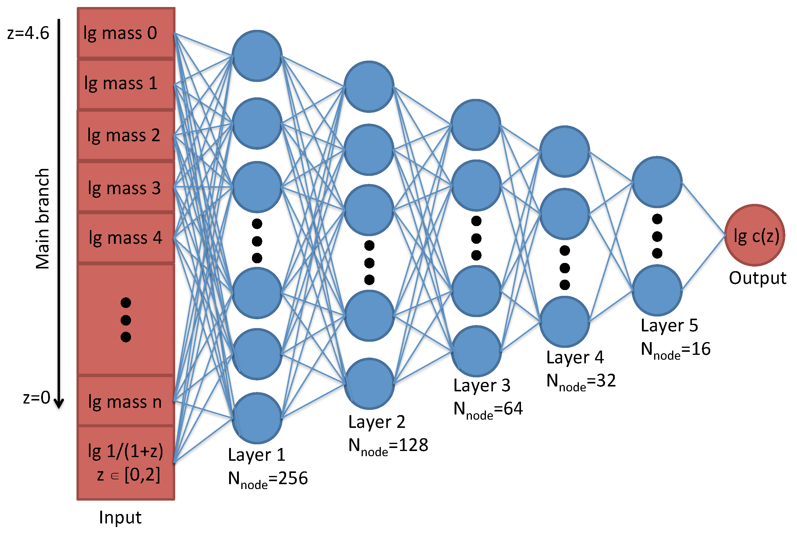
2.3. Neural Network Model

We employ an optimal framework for the rapid implementation of a neural network using the Python package PyTorch [42] to predict halo concentrations in this work. The structure of the neural network is illustrated in Figure 1, which includes the input layer, hidden layer, output layer, and the number of neurons in each layer.

There are 124 neurons in the input layer, which include the halo mass ($\log M_{\mathrm{vir}}$) corresponding to 123 snapshots along the MAH and one predicted redshift z (with $z\in [0,2]$, corresponding to 103 snapshots. Here, we convert z to $\log (1/(1+z\left)\right)$ to avoid $\log 0$ when $z=0$). In total, the SimA dataset comprises 721,000 datasets, derived from 7000 MAHs multiplied by 103 redshift values. The first 618,000 datasets are used as the TrainDataset to build the model, while the remaining 103,000 serve as the ValidationDataset for multiple iterations to adjust the model’s parameters. The 1480 MAHs from SimB consist of a total of 152,440 TestDataset, which are used only once to verify the model’s generalization performance.

We normalize the input parameters using the formula $y=(x-\mu )/\sigma$, where x is the value of each input neuron, and $\mu$ and $\sigma$ represent the mean and standard deviation of the corresponding neurons, respectively. The normalized input parameters y pass through five hidden layers, with the number of nodes in each layer being 256, 128, 64, 32, and 16, respectively. We apply the ReLU activation function ($f\left(y\right)=max(0,y)$), which enhances the nonlinearity of the neural network [43]. The mean squared error loss function [44] is used to measure the error between the actual and predicted values,

$$L=\sum _{\mathrm{i}=0}^{\mathrm{BatchSize}}{(\log c_{\mathrm{i},\mathrm{sim}}-\log c_{\mathrm{i},\mathrm{pred}})}^2,$$

(5)

where $c_{\mathrm{i},\mathrm{sim}}$ is the actual concentration of i-th TrainDataset and $c_{\mathrm{i},\mathrm{pred}}$ is the concentration predicted by the neural network model, The BatchSize is set to 256 to improve the training speed and enhance randomness in the training process. The weight of each node is updated using back propagation, and the Adam optimizer [45] is employed for faster convergence to find the optimal solution after each step within each batch. The output layer exports the final predicted halo concentration at z. The neural network model is trained 100 times with a learning rate of 0.001. After each step, we use the ValidationDataset to calculate the root mean square error (RMSE, $\sqrt{L}$) until the value converges, and we save this network as our model for the next section.

3. Results

To assess potential issues with our neural network model, we examined the well-known halo $c-M$ relation to determine whether the model can reproduce universal results: as halo mass increases, halo concentration decreases (see, e.g., [12,13,15,16], etc.). In Figure 2, we plot the $c-M$ relation at $z=0$, comparing the fitted NFW profile of haloes in the simulation (black curve) with predictions from our model (red curve). The neural network model closely reproduces the simulation results, supporting the aforementioned universal conclusion. In the residual panel, the median error of our model relative to the median error from the simulation is mostly less than 2.5%. Only at the massive end does the error increase to about 5%, likely due to the smaller number of halo samples in this mass range.

While the statistical performance of halo concentrations obtained from the our model appears promising, we also sought to evaluate its accuracy on an individual halo. In Figure 3, we plot the halo concentrations measured from simulations (ValidationDataset in SimA and TestDataset in SimB) against those predicted by the our model at $z=0$. The left panel displays a scatter plot for the ValidationDataset (blue), featuring RMSE of 0.0868. The points are closely distributed along the diagonal $c_{\mathrm{sim}}$ = $c_{\mathrm{pred}}$, indicating high predictive accuracy for this dataset. In the middle panel, the model similarly demonstrates strong performance for the TestDataset, achieving an RMSE of 0.0845. The true concentration values and the model’s predictions show comparable accuracy for both datasets, with the blue and red points aligning closely along the $c_{\mathrm{sim}}$ = $c_{\mathrm{pred}}$ line. The right panel further illustrates robust agreement between the two contours. These findings emphasize the neural network model’s strong generalization capabilities, enabling it to accurately predict halo concentrations not only within the same simulation but also across different simulations. We also tested our model with varying initial condition realizations, and obtained similarly predictions.

For comparison with other works, we derive concentrations from halo mass accretion history using the models of Zhao et al. [23] and Giocoli et al. [24]. In the Zhao et al. model, halo concentrations may be related to the universe is age when the main progenitor first reaches 4% of its current mass,

$$c=4{\left\{1+{\left({\displaystyle \frac{t}{3.75t_{0.04}}}\right)}^{8.4}\right\}}^{1/8},$$

(6)

where $t_{0.04}$ is the universe is age at that time. The model proposed by Giocoli et al. includes one additional parameter compared to the Zhao et al. model,

$$\log c=\log 0.45\left\{4.23+{\left({\displaystyle \frac{t}{t_{0.04}}}\right)}^{1.15}+{\left({\displaystyle \frac{t}{t_{0.5}}}\right)}^{2.3}\right\},$$

(7)

where $t_{0.5}$ is the age of the universe when the main progenitor has accreted half of its current mass. The comparison results are shown in Figure 4. We first present the results of $z=0$ in the first row. The left panel presents results from Zhao et al. [23], with RMSE of 0.1282. The scatter points are distributed around the diagonal but exhibit significant spread. The middle panel shows results from Giocoli et al. [24], yielding RMSE of 0.1281, which displays a similar distribution to Zhao et al. [23]. In contrast, the right panel depicts results from this work, with RMSE of 0.0845. Here, the scatter points are more tightly clustered around the diagonal, indicating that the neural network model outperforms the previous methods in predicting halo concentrations at $z=0$, while the predictive performance of the other models is comparable, both show slight deviations from the $c_{\mathrm{sim}}$ = $c_{\mathrm{pred}}$ line. In stark contrast, the points predicted by our model closely align with the $c_{\mathrm{sim}}$ = $c_{\mathrm{pred}}$ line across both low and high concentrations, demonstrating the strong predictive power and robustness of our model. The second, third and fourth rows present the results of $z=0.5$, 1 and 2. We found that the predictive ability of the neural network model at these redshifts far exceeds that of the other two models. Specifically, at $z=2$ the Zhao et al. [23] model initializes the concentration of most haloes to 4, leading to unreliable predictions. Meanwhile, the Giocoli et al. [24] model tends to overestimate the concentration of haloes. In contrast, the scatter in our model remains reasonably distributed around the diagonal, indicating more reliable predictions. What makes our model more effective than the other two? This likely stems from the inclusion of more variables, which provides a richer input for the halo mass accretion history. In contrast, the Zhao et al. [23] model includes only one variable, $t_{0.04}$, while the Giocoli et al. [24] model uses two variables, $t_{0.04}$ and $t_{0.5}$. A more detailed mass accretion history leads to more accurate prediction of halo concentration.

We further extend the prediction capability of our model to high-redshift samples, and present the evolution of the RMSE with redshift in Figure 5. Both Zhao et al. [23] and Giocoli et al. [24] show similar RMSE values across different redshifts, with overall higher levels, indicating that these methods are less accurate in their predictions. Throughout the redshift range, the RMSE for our method remains consistently lower than that of the other two methods, decreasing as redshift decreases. The change in RMSE from $z=0$ to $z=2$ is more obvious than that of the other two models. One possible reason is that as redshift increases, the model learns progressively less information about the mass accretion from halo merger trees, leading to a reduction in predictive capability. In contrast, the other two models rely on fixed parameters, which results in their RMSE remaining relatively stable throughout the redshift range and consistently higher than that of our model. Overall, our model demonstrates consistently lower RMSE across redshifts, indicating superior predictive accuracy compared to the other models.

We evaluate the model’s ability to predict concentrations for snapshots not included in the simulation. Following the method outlined in Section 2.3, we train our model using half of the TrainDataset, sampled at equal intervals between $z=2$ and $z=0$. The trained model is then used to predict concentrations for half of the TestDataset snapshots within the same redshift range (blue line) and to track the RMSE evolution for the remaining TestDataset snapshots (red line) in Figure 6. The close alignment of the two lines demonstrates that the model operates continuously rather than discretely. Given any halo mass accretion history and a target redshift, the model reliably predicts halo concentration at that redshift. Although halving the size of the TrainDataset slightly reduces model performance, it still outperforms the predictive capabilities of the models proposed by Zhao et al. [23] and Giocoli et al. [24].

4. Conclusions and Outlook

Using the mass accretion histories of haloes from cosmological N-body simulations, we employ a deep learning neural network algorithm to predict the concentrations of individual dark haloes across various redshifts, achieving remarkable accuracy. Our key findings are summarized as follows:

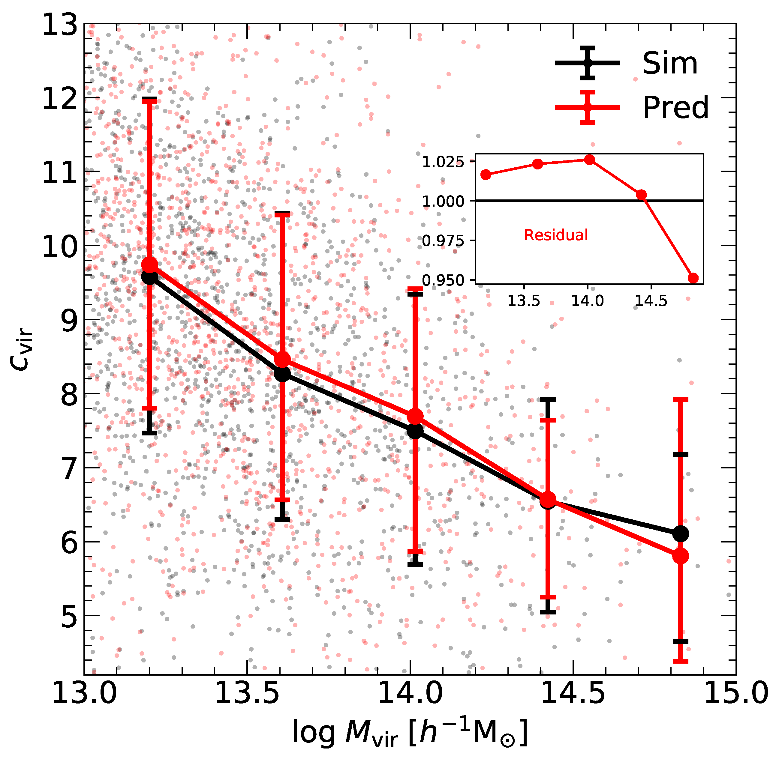
• The neural network model accurately reproduces the established relationship between halo mass and halo concentration at $z=0$.
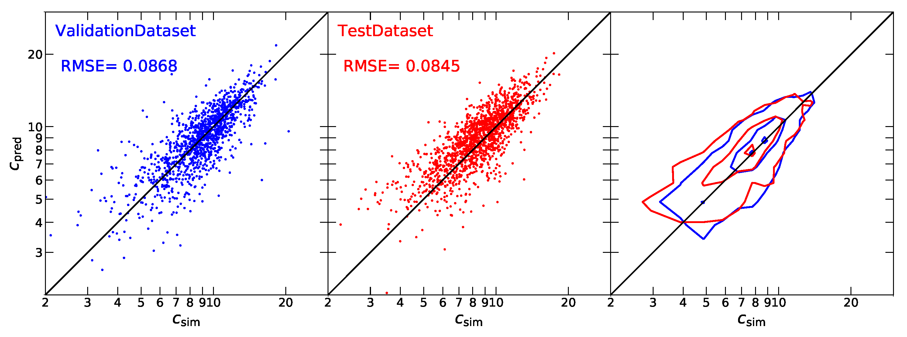
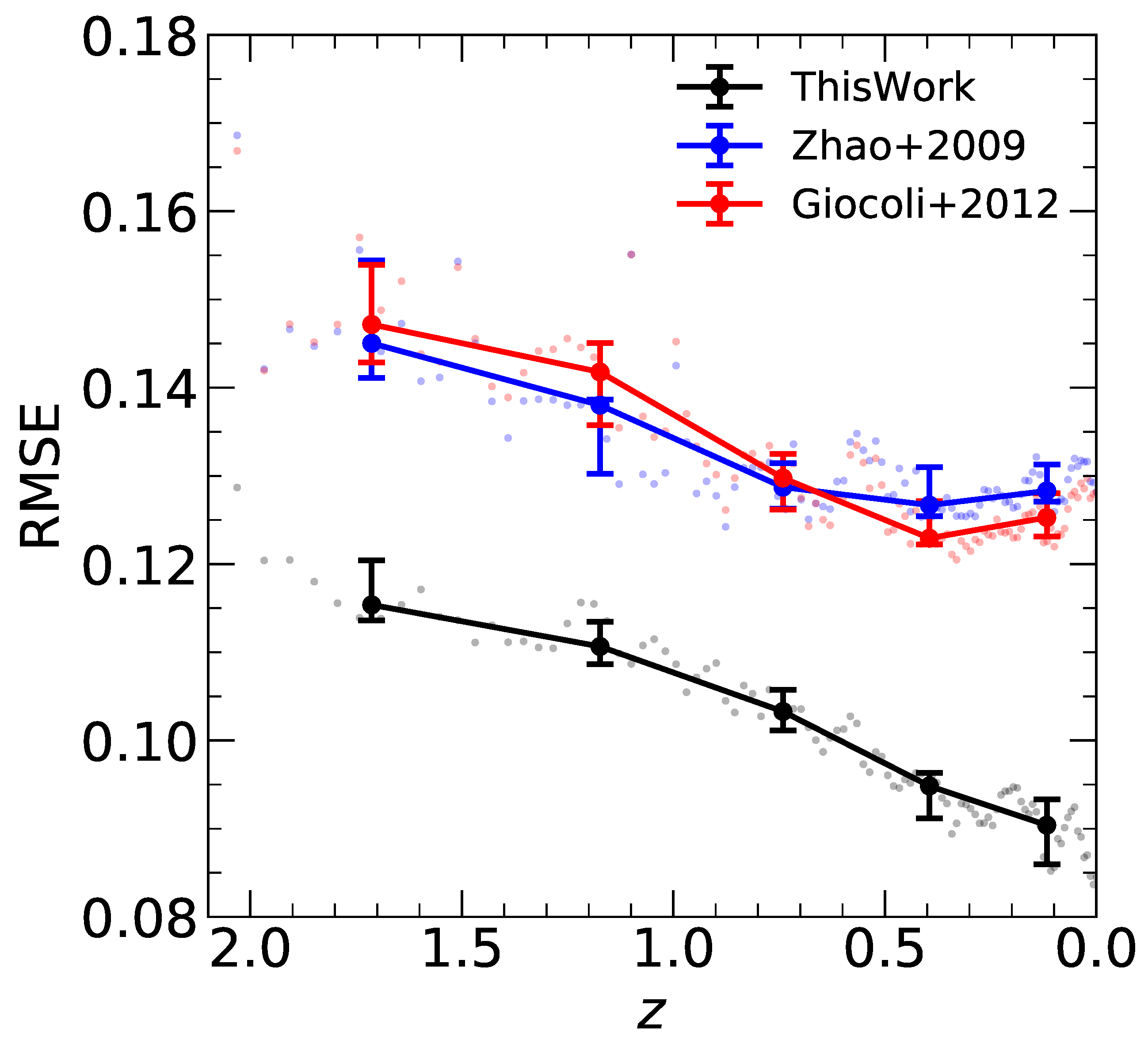
• When tested on a new simulation with a different initial condition realization, the trained model performs exceptionally well. At $z=0$, the RMSE between the actual and predicted concentrations is approximately 0.08, which is significantly lower than the RMSE of about 0.13 obtained from the models of Zhao et al. [23] and Giocoli et al. [24].
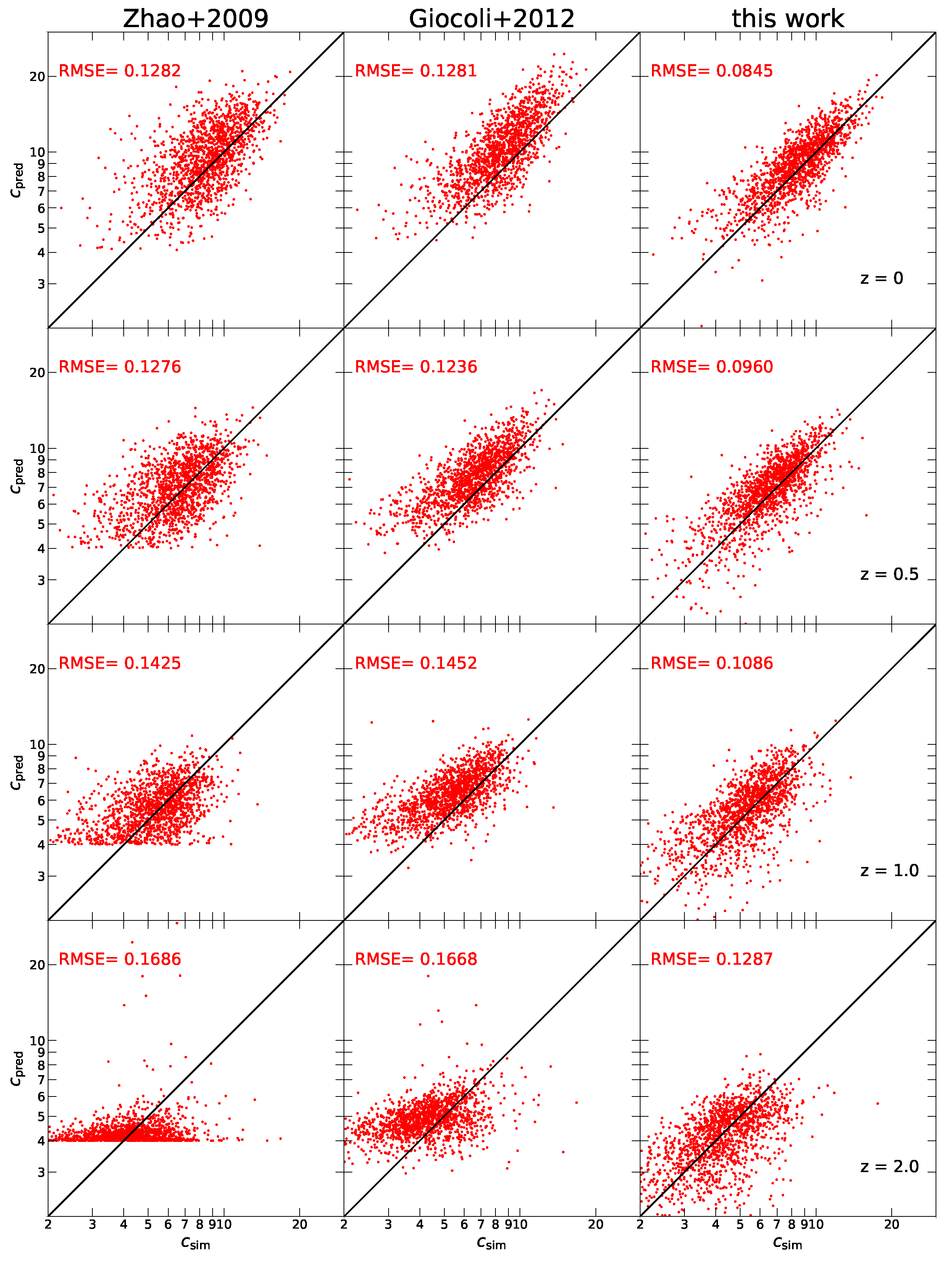
• The model demonstrates robust predictive capability at other redshifts. Within the range $z=2$ to $z=0$, although the RMSE increases with redshift and prediction accuracy declines, the neural network consistently achieves substantially lower RMSE values compared to the models by Zhao et al. [23] and Giocoli et al. [24].
• The neural network model exhibits continuity in its predictions, enabling accurate estimation of halo concentrations for snapshots not explicitly included in the simulation.

Overall, our neural network model, trained on the mass accretion histories of haloes, demonstrates strong predictive power and robust performance. Given a merger tree and a target redshift, the model can reliably predict the concentration of individual dark matter haloes at that redshift.

In this paper, our model fixes the cosmological parameters, leading to significant improvements in the corresponding concentration predictions. However, halo concentrations are also influenced by other factors. In a future work, we plan to explore models with varying cosmological parameters (such as ${\mathrm{\Omega }}_{\mathrm{m}}$, ${\mathrm{\Omega }}_{\Lambda }$ and ${\sigma }_8$) and investigate different halo definitions to further demonstrate the superiority, scalability, and robustness of our model.

Our current training set has some limitations, as the halo mass range it covers is relatively narrow. Wang et al. [46] used cosmic zoom simulations to show that the mass-concentration relation, from the smallest Earth-mass haloes to the largest cluster-sized haloes, can be described by a single model [47,48]. In the future, we plan to run a large number of high-resolution cosmological simulations of different box sizes to expand our training set to include a broader mass range to better compare with these studies and explore the potential of neural networks to predict additional halo properties from their mass accretion histories.

References

1. Frenk, C.S.; White, S.D.M. Dark matter and cosmic structure. Ann. Der Phys. 2012, 524, 507–534. [Google Scholar] [CrossRef]
2. Angulo, R.E.; Hahn, O. Large-scale dark matter simulations. Living Rev. Comput. Astrophys. 2022, 8, 1. [Google Scholar] [CrossRef]
3. Okoli, C. Dark matter halo concentrations: A short review. arXiv 2017, arXiv:1711.05277. [Google Scholar]
4. Jiang, F.; Dekel, A.; Kneller, O.; Lapiner, S.; Ceverino, D.; Primack, J.R.; Faber, S.M.; Macciò, A.V.; Dutton, A.A.; Genel, S.; et al. Is the dark-matter halo spin a predictor of galaxy spin and size? Mon. Not. R. Astron. Soc. 2019, 488, 4801–4815. [Google Scholar] [CrossRef]
5. Mo, H.J.; Mao, S.; White, S.D.M. The formation of galactic discs. Mon. Not. R. Astron. Soc. 1998, 295, 319–336. [Google Scholar] [CrossRef]
6. Yang, H.; Gao, L.; Frenk, C.S.; Grand, R.J.J.; Guo, Q.; Liao, S.; Shao, S. The galaxy size to halo spin relation of disc galaxies in cosmological hydrodynamical simulations. Mon. Not. R. Astron. Soc. 2023, 518, 5253–5259. [Google Scholar] [CrossRef]
7. Runge, J.; Walker, S.A.; Mirakhor, M.S. The unusually high dark matter concentration of the galaxy group NGC 1600. Mon. Not. R. Astron. Soc. 2022, 509, 2647–2653. [Google Scholar] [CrossRef]
8. Minor, Q.; Gad-Nasr, S.; Kaplinghat, M.; Vegetti, S. An unexpected high concentration for the dark substructure in the gravitational lens SDSSJ0946+1006. Mon. Not. R. Astron. Soc. 2021, 507, 1662–1683. [Google Scholar] [CrossRef]
9. Enzi, W.J.R.; Krawczyk, C.M.; Ballard, D.J.; Collett, T.E. The overconcentrated dark halo in the strong lens SDSS J0946+1006 is a subhalo: Evidence for self interacting dark matter? arXiv 2024, arXiv:2411.08565. [Google Scholar]
10. Macciò, A.V.; Dutton, A.A.; van den Bosch, F.C. Concentration, spin and shape of dark matter haloes as a function of the cosmological model: WMAP1, WMAP3 and WMAP5 results. Mon. Not. R. Astron. Soc. 2008, 391, 1940–1954. [Google Scholar] [CrossRef]
11. Ludlow, A.D.; Navarro, J.F.; Angulo, R.E.; Boylan-Kolchin, M.; Springel, V.; Frenk, C.; White, S.D.M. The mass-concentration-redshift relation of cold dark matter haloes. Mon. Not. R. Astron. Soc. 2014, 441, 378–388. [Google Scholar] [CrossRef]
12. Neto, A.F.; Gao, L.; Bett, P.; Cole, S.; Navarro, J.F.; Frenk, C.S.; White, S.D.M.; Springel, V.; Jenkins, A. The statistics of Λ CDM halo concentrations. Mon. Not. R. Astron. Soc. 2007, 381, 1450–1462. [Google Scholar] [CrossRef]
13. Gao, L.; Navarro, J.F.; Cole, S.; Frenk, C.S.; White, S.D.M.; Springel, V.; Jenkins, A.; Neto, A.F. The redshift dependence of the structure of massive Λ cold dark matter haloes. Mon. Not. R. Astron. Soc. 2008, 387, 536–544. [Google Scholar] [CrossRef]
14. Klypin, A.A.; Trujillo-Gomez, S.; Primack, J. Dark Matter Halos in the Standard Cosmological Model: Results from the Bolshoi Simulation. Astrophys. J. 2011, 740, 102. [Google Scholar] [CrossRef]
15. Bhattacharya, S.; Habib, S.; Heitmann, K.; Vikhlinin, A. Dark Matter Halo Profiles of Massive Clusters: Theory versus Observations. Astrophys. J. 2013, 766, 32. [Google Scholar] [CrossRef]
16. Dutton, A.A.; Macciò, A.V. Cold dark matter haloes in the Planck era: Evolution of structural parameters for Einasto and NFW profiles. Mon. Not. R. Astron. Soc. 2014, 441, 3359–3374. [Google Scholar] [CrossRef]
17. Child, H.L.; Habib, S.; Heitmann, K.; Frontiere, N.; Finkel, H.; Pope, A.; Morozov, V. Halo Profiles and the Concentration-Mass Relation for a ΛCDM Universe. Astrophys. J. 2018, 859, 55. [Google Scholar] [CrossRef]
18. Diemer, B.; Joyce, M. An Accurate Physical Model for Halo Concentrations. Astrophys. J. 2019, 871, 168. [Google Scholar] [CrossRef]
19. Ishiyama, T.; Prada, F.; Klypin, A.A.; Sinha, M.; Metcalf, R.B.; Jullo, E.; Altieri, B.; Cora, S.A.; Croton, D.; de la Torre, S.; et al. The Uchuu simulations: Data Release 1 and dark matter halo concentrations. Mon. Not. R. Astron. Soc. 2021, 506, 4210–4231. [Google Scholar] [CrossRef]
20. Bullock, J.S.; Kolatt, T.S.; Sigad, Y.; Somerville, R.S.; Kravtsov, A.V.; Klypin, A.A.; Primack, J.R.; Dekel, A. Profiles of dark haloes: Evolution, scatter and environment. Mon. Not. R. Astron. Soc. 2001, 321, 559–575. [Google Scholar] [CrossRef]
21. Wechsler, R.H.; Bullock, J.S.; Primack, J.R.; Kravtsov, A.V.; Dekel, A. Concentrations of Dark Halos from Their Assembly Histories. Astrophys. J. 2002, 568, 52–70. [Google Scholar] [CrossRef]
22. Zhao, D.H.; Jing, Y.P.; Mo, H.J.; Börner, G. Mass and Redshift Dependence of Dark Halo Structure. Astrophys. J. 2003, 597, L9–L12. [Google Scholar] [CrossRef]
23. Zhao, D.H.; Jing, Y.P.; Mo, H.J.; Börner, G. Accurate Universal Models for the Mass Accretion Histories and Concentrations of Dark Matter Halos. Astrophys. J. 2009, 707, 354–369. [Google Scholar] [CrossRef]
24. Giocoli, C.; Tormen, G.; Sheth, R.K. Formation times, mass growth histories and concentrations of dark matter haloes. Mon. Not. R. Astron. Soc. 2012, 422, 185–198. [Google Scholar] [CrossRef]
25. Fluke, C.J.; Jacobs, C. Surveying the reach and maturity of machine learning and artificial intelligence in astronomy. WIREs Data Min. Knowl. Discov. 2020, 10, e1349. [Google Scholar] [CrossRef]
26. Sen, S.; Agarwal, S.; Chakraborty, P.; Singh, K.P. Astronomical big data processing using machine learning: A comprehensive review. Exp. Astron. 2022, 53, 1–43. [Google Scholar] [CrossRef]
27. Aragon-Calvo, M.A. Classifying the large-scale structure of the universe with deep neural networks. Mon. Not. R. Astron. Soc. 2019, 484, 5771–5784. [Google Scholar] [CrossRef]
28. Sun, S.; Liao, S.; Guo, Q.; Wang, Q.; Gao, L. HIKER: A halo-finding method based on kernel-shift algorithm. arXiv 2019, arXiv:1909.13301. [Google Scholar] [CrossRef]
29. Wadekar, D.; Villaescusa-Navarro, F.; Ho, S.; Perreault-Levasseur, L. HInet: Generating Neutral Hydrogen from Dark Matter with Neural Networks. Astrophys. J. 2021, 916, 42. [Google Scholar] [CrossRef]
30. Mao, T.X.; Wang, J.; Li, B.; Cai, Y.C.; Falck, B.; Neyrinck, M.; Szalay, A. Baryon acoustic oscillations reconstruction using convolutional neural networks. Mon. Not. R. Astron. Soc. 2021, 501, 1499–1510. [Google Scholar] [CrossRef]
31. Maltz, M.G.A.; Thomas, P.A.; Lovell, C.C.; Roper, W.J.; Vijayan, A.P.; Irodotou, D.; Liao, S.; Seeyave, L.T.C.; Wilkins, S.M. First Light and Reionisation Epoch Simulations (FLARES) XVII: Learning the galaxy-halo connection at high redshifts. arXiv 2024, arXiv:2410.24082. [Google Scholar] [CrossRef]
32. Springel, V. The cosmological simulation code GADGET-2. Mon. Not. R. Astron. Soc. 2005, 364, 1105–1134. [Google Scholar] [CrossRef]
33. Eisenstein, D.J.; Hu, W. Baryonic Features in the Matter Transfer Function. Astrophys. J. 1998, 496, 605–614. [Google Scholar] [CrossRef]
34. Liao, S. An alternative method to generate pre-initial conditions for cosmological N-body simulations. Mon. Not. R. Astron. Soc. 2018, 481, 3750–3760. [Google Scholar] [CrossRef]
35. Zhang, T.; Liao, S.; Li, M.; Zhang, J. Numerical convergence of pre-initial conditions on dark matter halo properties. Mon. Not. R. Astron. Soc. 2021, 507, 6161–6176. [Google Scholar] [CrossRef]
36. Zhang, T.; Liao, S.; Li, M.; Gao, L. The optimal gravitational softening length for cosmological N-body simulations. Mon. Not. R. Astron. Soc. 2019, 487, 1227–1232. [Google Scholar] [CrossRef]
37. Davis, M.; Efstathiou, G.; Frenk, C.S.; White, S.D.M. The evolution of large-scale structure in a universe dominated by cold dark matter. Astrophys. J. 1985, 292, 371–394. [Google Scholar] [CrossRef]
38. Han, J.; Cole, S.; Frenk, C.S.; Benitez-Llambay, A.; Helly, J. HBT+: An improved code for finding subhaloes and building merger trees in cosmological simulations. Mon. Not. R. Astron. Soc. 2018, 474, 604–617. [Google Scholar] [CrossRef]
39. Bryan, G.L.; Norman, M.L. Statistical Properties of X-Ray Clusters: Analytic and Numerical Comparisons. Astrophys. J. 1998, 495, 80–99. [Google Scholar] [CrossRef]
40. Navarro, J.F.; Frenk, C.S.; White, S.D.M. The Structure of Cold Dark Matter Halos. Astrophys. J. 1996, 462, 563. [Google Scholar] [CrossRef]
41. Navarro, J.F.; Frenk, C.S.; White, S.D.M. A Universal Density Profile from Hierarchical Clustering. Astrophys. J. 1997, 490, 493–508. [Google Scholar] [CrossRef]
42. Paszke, A.; Gross, S.; Massa, F.; Lerer, A.; Bradbury, J.; Chanan, G.; Killeen, T.; Lin, Z.; Gimelshein, N.; Antiga, L.; et al. Pytorch: An imperative style, high-performance deep learning library. Adv. Neural Inf. Process. Syst. 2019, 32. [Google Scholar]
43. Nair, V.; Hinton, G.E. Rectified linear units improve restricted boltzmann machines. In Proceedings of the 27th International Conference on Machine Learning (ICML-10), Haifa, Israel, 21–24 June 2010; pp. 807–814. [Google Scholar]
44. Rumelhart, D.E.; Hinton, G.E.; Williams, R.J. Learning representations by back-propagating errors. Nature 1986, 323, 533–536. [Google Scholar] [CrossRef]
45. Kingma, D.P. Adam: A method for stochastic optimization. arXiv 2014, arXiv:1412.6980. [Google Scholar]
46. Wang, J.; Bose, S.; Frenk, C.S.; Gao, L.; Jenkins, A.; Springel, V.; White, S.D.M. Universal structure of dark matter haloes over a mass range of 20 orders of magnitude. Nature 2020, 585, 39–42. [Google Scholar] [CrossRef]
47. Zheng, H.; Bose, S.; Frenk, C.S.; Gao, L.; Jenkins, A.; Liao, S.; Liu, Y.; Wang, J. The abundance of dark matter haloes down to Earth mass. Mon. Not. R. Astron. Soc. 2024, 528, 7300–7309. [Google Scholar] [CrossRef]
48. Liu, Y.; Gao, L.; Bose, S.; Frenk, C.S.; Jenkins, A.; Springel, V.; Wang, J.; White, S.D.M.; Zheng, H. The mass accretion history of dark matter haloes down to Earth mass. Mon. Not. R. Astron. Soc. 2024, 527, 11740–11750. [Google Scholar] [CrossRef]
Figure 1. The schematic of our neural network is presented here. Red squares represent the input layer neurons, which take the MAH and the desired z as input parameters. The blue circles indicate the neurons in the hidden layers; there are five layers in total, with the number of neurons in each layer denoted by N node . The red circle represents the single neuron in the output layer, which outputs the halo concentration at z.
Universe 11 00037 g001
Figure 2. The halo concentration–mass relation at z = 0 is derived from fitting the NFW profile (black) and utilizing a neural network model (red). The scatter points in the background indicate individual haloes, whereas the larger points connected by lines represent the median values. Error bars denote the 16th and 84th percentiles. The small panel in the upper right displays the residuals between the predicted results of our model and the simulation results.
Universe 11 00037 g002
Figure 3. A comparison of the measured concentrations with those predicted by our model in SimA and SimB at z = 0 . Blue points represent the ValidationDataset from SimA, while red points denote the TestDataset from SimB. The contours enclose 10%, 50%, and 90% of the haloes, providing a visual representation of concentration distribution. The solid black lines indicate the c sim = c pred in each panel, highlighting the accuracy of the model’s predictions. These highlight the neural network model’s ability to generalize effectively, allowing it to predict halo concentrations accurately across different simulations.
Universe 11 00037 g003
Figure 4. Similar to Figure 3, except that concentrations predicted by models by Zhao et al. [23] (denoted as "Zhao+2009", left column), Giocoli et al. [24] (denoted as "Giocoli+2012", middle column), and neural network in TestDataset at different redshifts. This demonstrates the model’s robust predictive ability across different redshifts.
Universe 11 00037 g004
Figure 5. The median relationship between the RMSE of the actual and predicted concentrations as a function of redshift. Black, blue, and red lines show results of neural network, Zhao, and Giocoli models, respectively. Error bars indicate the 16th and 84th percentiles. The consistently lower RMSE of our model across redshifts suggests its superior predictive accuracy over the other models.
Universe 11 00037 g005
Figure 6. Similarly to Figure 5, the black line is identical to the one in the previous figure. The blue line represents the predictions on the TestDataset using the model trained on half of the snapshots between z = 2 and z = 0 . Additionally, the red line shows the predictions made by the model from the blue line on the halo concentrations corresponding to the remaining half of the TestDataset snapshots. This illustrates our model’s ability to accurately predict halo concentrations for snapshots not present in the simulation.
Universe 11 00037 g006
Disclaimer/Publisher’s Note: The statements, opinions and data contained in all publications are solely those of the individual author(s) and contributor(s) and not of MDPI and/or the editor(s). MDPI and/or the editor(s) disclaim responsibility for any injury to people or property resulting from any ideas, methods, instructions or products referred to in the content.