Abstract
A classical three-body problem with two planets moving around a central star of variable mass on quasi-periodic orbits is considered. The bodies are assumed to attract each other according to Newton’s law of universal gravitation. The star loses its mass anisotropically, and this leads to the appearance of reactive forces. The problem is analyzed in the framework of Newtonian’s formalism, and equations of motion are derived in terms of the osculating elements of aperiodic motion on quasi-conic sections. As equations of motion are not integrable, the perturbation theory is applied with the perturbing forces expanded into power series in terms of eccentricities and inclinations, which are assumed to be small. Averaging these equations over the mean longitudes of the planets in the absence of mean-motion resonances, we obtain the differential equations describing the long-term evolution of orbital elements. Numerical solutions to the evolution equations are obtained and analyzed for three different three-body systems. The obtained results demonstrate clearly that variability of masses may influence essentially the secular evolution of the orbital elements. All the relevant symbolic and numerical calculations are performed with the computer algebra system Wolfram Mathematica.
1. Introduction
The classical three-body problem is a famous model of celestial mechanics that describes the motion of three particles , , and of constant masses , , and , respectively, attracting each other according to Newton’s law of universal gravitation (e.g., see [1,2]). It may be applied to describe two planets orbiting a star, for example, or a planet with a satellite moving around a star like the Sun–Earth–Moon system (see [3]). As the three-body problem is not integrable, the system motion is usually investigated with the perturbation theory methods that have been developed quite well and can give approximate solutions to high degrees of accuracy (see, for example, [3,4,5,6]). If the body , for example, has a dominant mass, the other two bodies, and , move, in the first approximation, around on elliptic orbits as if they were attracted solely by the body . Each such orbit is described by the corresponding exact solution to the two-body problem and is determined by six constants that are uniquely determined from the initial positions and velocities of the bodies and are known as the orbital elements (see [2]).
The mutual gravitational attraction of the bodies and , which is usually at least an order of magnitude smaller than that of the body , disturbs their motion and forces the orbital elements to change (see [3,4]). As a result, elliptic orbits of the bodies and are not fixed but slowly rotate or precess in space and change their orientation and shape. The most famous example is an advance of Mercury’s perihelion that is not fixed but moves round in the direction of Mercury’s motion (see [7]). However, numerous investigations have shown that the observed advance in the perihelion of Mercury is greater than could be obtained even by adding together the gravitational effects of the known planets in the solar system.
There were different approaches to account for the discrepancy between the observed value of the advance of Mercury’s perihelion and the theoretical value predicted from Newtonian theory. For example, additional forces were added to the basic inverse square gravitational force of Newton or additional matter in the solar system that had not yet been discovered and whose influence had not been taken into account (for details, see [7]). Finally, a more general model of gravity was given by Einstein’s general theory of relativity that completely accounted for this discrepancy. Moreover, this agreement between the theoretical predictions and observations was an essential confirmation of the general theory of relativity. However, this does not exclude the possibility of looking for more realistic models taking into account such factors as the variability of the system’s physical parameters, for example, which may provide a refinement of results obtained in the framework of the classical many-body problem.
It should be emphasized that all parameters in the classical three-body problem are usually considered to be constant. However, observational astronomy shows that real-life celestial bodies are non-stationary; some of their characteristics, such as mass, for example, may change with time (e.g., see [8,9,10]). As the force of gravitational attraction of two bodies is proportional to their masses, variability of masses may influence substantially the dynamical evolution of the bodies, which makes a study of such systems highly relevant (see [11,12,13,14,15,16]). The mass of a star, for example, decreases considerably during its lifetime due to corpuscular and light emission, and this mass loss may play an important role in the evolution of the three-body system (see [17,18,19,20,21,22,23,24,25]). Taking into account the variability of the system parameters enables us to make the model more realistic and to describe the motion of celestial bodies more accurately.
Note that non-stationarity complicates substantially the corresponding mathematical models of the body’s motion. In the simplest case it is assumed that masses of the bodies vary isotropically and the momentum of escaping (or incident) mass of each body is equal to the momentum that this mass would have if it were attached to the moving body at its center of mass. Then the equations of motion of the bodies look similar to the case of constant masses (see [26,27,28,29]). However, even the two-body problem becomes non-integrable in the case of variable masses; only for some specific mass variation laws can its exact analytical solution be found (see [30,31,32,33,34,35,36,37,38,39]).
The general case of the two-body problem with variable masses may be investigated with application of the perturbation theory (see [13,40]). In [41], we derived the differential equations determining the perturbed motion of the bodies in terms of the osculating elements of aperiodic motion on a quasi-conic section and showed that variability of mass leads to the change in the orbital elements with time even in the framework of the two-body problem. Therefore, one can expect to obtain better agreement of the results of calculations of the secular perturbations of the orbital elements and their observed values if the variability of the masses is taken into account together with the mutual interaction of the bodies. The study of such models is usually associated with cumbersome symbolic calculations, for which it is expedient to use computer algebra systems, for example, Wolfram Mathematica [42].
Our goal is to investigate the effect of the isotropic and anisotropic mass variation on the dynamical evolution of the two-planet system consisting of a star orbited by two planets. We consider the case when the trajectory of the body of smaller mass is located inside of the trajectory of the greater body and their trajectories do not intersect. It is assumed that the star ejects its mass anisotropically, and due to this, it is acted on by the reactive force. The bodies, and , may also change their masses anisotropically, and the corresponding reactive forces are defined in their orbital frames of reference. In contrast to [16,40], here we derive the differential equations determining the perturbed motion of the bodies in the framework of Newton’s formalism in terms of the osculating elements of aperiodic motion on quasi-conic sections; the details of the derivation of these equations may be found in [43,44]. Here, we also assume that the star ejects its mass mostly in the direction of the more massive body , and due to this, one needs to repeat all the calculations described in [43,44] to derive equations of the perturbed motion. For the special case of small eccentricities and inclinations of the orbits, the perturbing forces are expanded into power series in small parameters up to the first-order terms. Then the equations of the perturbed motion are averaged over the mean longitudes to obtain the differential equations describing the evolution of orbital elements over long periods of time. Then we solve the evolutionary equations numerically for three different three-body systems. Comparison of the obtained results with the case of constant masses demonstrates clearly that variability of masses may essentially modify the secular evolution of the orbital elements. All the relevant symbolic and numerical calculations we carry out with the computer algebra system Wolfram Mathematica [42].
2. Model Description
Consider a system of three bodies , , and of variable masses , , and , respectively, attracting each other according to Newton’s law of universal gravitation. We assume that the body has a dominant mass and two bodies , move around along quasi-elliptic orbits that do not intersect. We assume also that masses of all bodies may change anisotropically, and due to this, the bodies are acted on by the reactive forces (see [45]). Denoting the position vectors of the bodies , relative to by and applying Newton’s second law, the equations of motion are written as (see [13,43,44])
where G is the gravitational constant, , and the distance between and is . The last term in Equation (1) describes the reactive forces acting on the bodies and and is given by
where is the relative velocity of the particles leaving the body or falling on it. It is assumed that the relative velocity is a given function of time for each body; if the body mass changes isotropically, then and the corresponding reactive force does not arise.
For , the equations of motion in Equation (1) look similar to the case of constant masses and are not integrable (see [2,3]). Moreover, neglecting the right-hand side in Equation (1), we obtain the two-body problem that is not integrable as well because of the dependence of the masses on time (see [41]). Therefore, a general solution to the two-body problem with variable masses that could be used as an unperturbed solution in the three-body problem under consideration is absent. However, one can modify the two-body problem in such a way that its general solution exists and is independent of the masses’ variation law. Indeed, let us rewrite Equation (1) as
where
The functions in Equations (3) and (4) are given by
where and are the masses of the bodies at the initial instant of time. These functions are determined by the laws of masses variation and may be arbitrary twice differentiable functions. Note that the function is determined by a sum of two masses and it may remain constant if , in spite of the dependence of each mass on time. Such a situation takes place in the case of mass transfer in a double system, for example, when and two bodies move along the Keplerian orbits (see [38]).
It is quite obvious that Equation (3) coincides with original Equation (1) because the same term is added to the left- and the right-hand sides of Equation (1). However, Equation (3) becomes integrable if their right-hand sides are replaced by zero or . Actually, at , the two parts of Equation (3) become independent of each other, and each of them has an exact solution that describes aperiodic motion of the body on a quasi-conic section (see [13]); the correspondent solution is
where the true anomaly is determined by the differential equation
and
The constants and in (5), (6) are analogs of the well-known Kepler orbital elements (see [2,3,13]) and are determined from the initial conditions of motion. The true anomaly characterizes the position of the body on the orbit; introducing an analog of the eccentric anomaly by the relation
we obtain the known Kepler equation
where the mean anomaly is given by
and . The functions have the form
By in Equation (9) we denote an analog of the time when the body passes through the pericenter (e.g., see [2,3]).
One can readily see that in the case of the solution in Equation (5), it reduces to the corresponding solution to the two-body problem with constant masses, and the mean anomaly becomes a linear function of time as (see Equations (9) and (10)). If the laws of masses variation are given, the function defines the mean anomaly , and Equations (7) and (8) enable us to find the eccentric anomaly and true anomaly as functions of time. Therefore, solution in Equation (5) describes the motion of the body on a quasi-conic section in terms of the time and 6 constants of integration , and , which are the analogs of the Keplerian orbital elements (see [2,13]). In contrast to the case of constant masses, this motion of the body is aperiodic because of the scale factor in Equation (5) and the nonlinear dependence of the mean anomaly on time (see Equation (9)). It should be emphasized also that the orbital elements in Equation (5) differ from the Keplerian orbital elements defining the ellipse. However, geometrically they are almost identical, at least over the finite time intervals over which observations are made, since the masses of celestial bodies change very slowly in reality. A comparison of these elements and their meaning has been discussed in our paper [16].
Note that Equation (5) does not yield a physical trajectory of the body that could be obtained in the case of absence of perturbations when the right-hand side of Equation (1) is set to zero. Equation (5) gives only an approximation for such a physical trajectory because the left-hand side of Equation (3) determining this solution for contains an additional term. From the other side, in the case of variable masses, the perturbing force in Equation (3) is not equal to zero even if we neglect the first term in Equation (4). This term describes the mutual attraction of the bodies and and is the only reason for the dependence of orbital elements on time in the case of constant masses. Note that an anisotropy of mass variation leads to the appearance of the reactive forces in Equation (2), which also contribute to the perturbing force in Equation (4). Although the masses of celestial bodies usually change very slowly (see [19,23,24]), and so the second and third terms in the expression for perturbing force in Equation (4) are quite small in some cases, their influence on the system motion may be significant (see [41]). Therefore, changing the masses of the bodies may modify the secular evolution of their orbital elements and should be taken into account in order to describe their motion more precisely.
Equations of the Perturbed Motion
As in the case of constant masses, the orbital elements , and become functions of time if the perturbing forces are taken into account. The differential equations determining these functions may be derived similarly to the case of constant masses (e.g., see [1,2]). We assume that the perturbed solution , , to Equation (3) at time t is given by Equation (5) in terms of the instantaneous orbital elements at t. Additionally, the corresponding components of the velocities , , are equal to the partial derivatives of Equation (5) with respect to time. Naturally, by virtue of this definition, the resulting solution to Equation (3) is determined by curves of Equation (5), tangent to the physical trajectories. Thus, although the orbital elements determined by Equation (5) differ from Keplerian orbital elements, they may be considered as the osculating elements. This is why we say that we look for a perturbed solution to Equation (3) in terms of the osculating elements of aperiodic motion along quasi-conical sections determined by Equation (5). The corresponding calculations are quite cumbersome and are described in detail in our papers [43,44].
Repeating the calculations, we finally obtain the system of differential equations determining the dependence of the orbital elements on time in the form of Lagrange’s planetary equations.
The forces , , and in the right-hand sides of Equations (11)–(16) are the radial, transversal and normal components of the forces , respectively, determined by Equation (4). To write out these forces explicitly, we need to define the unit vectors , , and along the radial, transversal, and normal directions, respectively, for each body . Using the solution (5), we easily obtain
To compute the reactive forces given by Equation (2), we need to introduce some assumption relating to the direction of the relative velocities of particles leaving the body or falling on it. Here, we assume that the body has much greater mass than body , and due to this, the star loses its mass, ejecting particles mostly in the direction of body . Therefore, vector has only one non-zero component directed along vector , while its transversal and normal components are zero. Denoting the components of the relative velocities of particles leaving the body or falling on it along the radial, transversal, and normal directions in the orbital system of coordinates related to the body by , , and , respectively, and using Equations (2) and (4), we obtain for the first body
Similarly, denoting the components of the relative velocities of particles leaving the body or falling on it along the radial, transversal, and normal directions in the orbital system of coordinates related to the body by , , and , we obtain the radial, transversal, and normal components of the force in the form
Recall that the relative velocities , and in Equations (20) and (21) of the particles leaving the bodies or falling on them are assumed to be given in the orbital coordinate systems related to the bodies and . If the laws of masses variation are given, Equations (11)–(16) completely determine the perturbed motion of the bodies .
3. Evolutionary Equations
Differential Equations (11)–(16) describe the perturbed motion of the bodies in terms of the osculating orbital elements, but they are not integrable, and their exact solution cannot be written in closed form. Of course, one could find their numerical solution, which describes the orbital elements of the bodies as functions of time. However, due to the orbital motion of the bodies and around the parent star, ; the right-hand sides of Equations (11)–(16) include many terms describing short-period oscillations. Therefore, to obtain the solution with high precision, one needs to choose a very small step size or to use an adaptive step size method, and this increase the time of calculation substantially. As we are interested in the long-term behavior of the system, it will be necessary to perform additional calculations in order to extract a secular part of the solution. At the same time, the long-term evolution of the orbital elements is the most interesting for applications in celestial mechanics.
It should be noted that in many problems of celestial mechanics, eccentricities and inclinations of body orbits are small (see [1,2,3]). Here, we consider this practically important case of small eccentricities and inclinations and expand the right-hand sides of Equations (11)–(16) in power series in these parameters. Note that applying the computer algebra system Wolfram Mathematica (see [42]), one can calculate such expansions with any required accuracy, but the corresponding expressions become very cumbersome in higher-order terms. Here, we restrict ourselves to computations up to the first order and obtain the differential equations for the orbital elements (all the details can be found in [43,44]). Assuming that trajectories of the bodies and do not intersect and averaging these equations over their mean longitudes in the absence of mean-motion resonances, we obtain the differential equations describing the secular evolution of the orbital elements in the form
where
and are the Laplace coefficients (see [3,43,44]). As orbital elements of the bodies are assumed to satisfy the conditions , the arguments of the Laplace coefficients in Equations (22)–(32) are smaller than 1.
Note that we do not consider the averaged Equation (16) here because, due to averaging the equation with respect to the mean longitudes, information about the location of the bodies on the orbits is lost. So we can analyze only slow changes in the orbital elements , , , , and in time determined by Equations (22)–(31). Although we take into account only linear terms in the power expansions of the right-hand sides of Equations (11)–(16) in terms of eccentricities and inclinations , the evolutionary Equations (22)–(32) are very complicated, and we cannot find their solution in symbolic form. However, we can choose some realistic laws of the masses’ variations and find numerical solutions to the evolutionary equations. In this way we can investigate the influence of the masses’ variation on the secular evolution of the two-planet system.
4. Results
In order to investigate an influence of masses change on the dynamic evolution of the system, we choose some realistic values for the system parameters and solve Equations (22)–(31) numerically. To simplify the calculations, it is convenient to use the dimensionless variables. For example, we use initial values of the semi-major axis and the mass of body as units of distance and mass, respectively, and define dimensionless distance , mass and time by
As a test system, we consider two three-body systems, namely, Sun–Mercury–Venus and Sun–Mercury–Jupiter, as bodies , , and , respectively. According to different estimates, the Sun loses its mass at the rate per year (see [18,24,25]), but this mass loss is usually not taken into account in studying the orbital evolution of the planets (see [23]). As the Sun exists in a main-sequence phase of its evolution, it is natural to assume that the mass of the star decreases according to the Eddington–Jeans law (see [46,47])
Here we consider the case of and choose the dimensionless coefficient = 1/50,000,000. Masses of the planets and are assumed to be constant.
We also choose the following initial values for orbital elements of the Sun, Mercury and Venus (see [2])
Initial values for orbital elements of Jupiter are (see [2])
For each three-body system we have considered three cases. First, all the masses are constant. In this case, we have the classical three-body problem, and our solutions to Equations (22)–(31) correspond to the known results (see [2,3]). Second, we assume that the star loses its mass isotropically and there are no reactive forces. Third, we assume that the star ejects its mass mostly in the direction of the more massive planet and the relative velocity of the particles leaving the star .
The solutions have shown that in all cases the dimensionless semi-major axes and of both bodies, and , do not change with time. However, due to the scale factor in Equation (5), the real semi-major axes are increasing functions of time (see Figure 1) as the function increases because the star loses its mass.

Figure 1.
The Sun–Mercury–Venus: Semi-major axes of Mercury (solid line) and Venus (dashed line).
Dependence on time of the other four orbital elements, namely, the eccentricity , the inclination , the longitude of ascending node , and the argument of pericenter for planets and are shown in Figure 2, Figure 3, Figure 4, Figure 5, Figure 6, Figure 7, Figure 8 and Figure 9. We use the following notations: In the case of constant masses, the corresponding curve is shown as a dashed curve; in the case of isotropic mass change, the curves have a larger dashing; in the case of anisotropic mass change, when reactive force appears, the curves are solid.
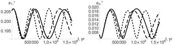
Figure 2.
Sun–Mercury–Venus: The eccentricities and (curves with small dashing—constant masses, curves with larger dashing—isotropic mass changes, solid curves—non-isotropic mass changes, ).

Figure 3.
Sun–Mercury–Jupiter: The eccentricities and (curves with small dashing—constant masses, curves with larger dashing—isotropic mass changes, solid curves—non-isotropic mass changes, ).
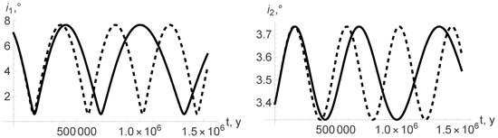
Figure 4.
Sun–Mercury–Venus: The inclinations and (curves with small dashing—constant masses, curves with larger dashing—isotropic mass changes, solid curves—non-isotropic mass changes, ).

Figure 5.
Sun–Mercury–Jupiter: The inclinations and (curves with small dashing—constant masses, curves with larger dashing—isotropic mass changes, solid curves—non-isotropic mass changes, ).
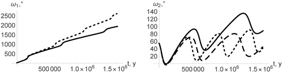
Figure 6.
Sun–Mercury–Venus: Arguments of pericenter (curves with small dashing—constant masses, curves with larger dashing—isotropic mass changes, solid curves—non-isotropic mass changes, ).
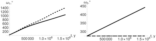
Figure 7.
Sun–Mercury–Jupiter: Arguments of pericenter (curves with small dashing—constant masses, curves with larger dashing—isotropic mass changes, solid curves—non-isotropic mass changes, ).
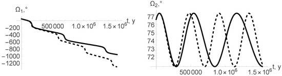
Figure 8.
Sun–Mercury–Mercury–Venus: Longitudes of ascending node (curves with small dashing—constant masses, curves with larger dashing—isotropic mass changes, solid curves—non-isotropic mass changes, ).
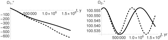
Figure 9.
Sun–Mercury–Mercury–Jupiter: Longitudes of ascending node (curves with small dashing—constant masses, curves with larger dashing—isotropic mass changes, solid curves—non-isotropic mass changes, ).
5. Discussion
It is important to remember that evolutionary Equations (22)–(31) describe the long-term behavior of the orbital elements , , , , and of two planets, and , orbiting the star . One can readily see that in the case of constant masses of the bodies, and , the time derivatives of the semi-major axes are equal to zero. Moreover, the semi-major axes may change only if the masses, and , vary anisotropically. As in the considered case, only the star loses its mass anisotropically; the functions remain constant. As far as the parts of Equation (5) are considered, the unperturbed one contains the scale factor ; the semi-major axes, in fact, are equal to the product , and their behavior is determined by the functions (see Figure 1).
Indeed, the function changes very slowly, and so the secular parts of the orbital elements determined by Equation (5) do not change noticeably during one revolution of the planets. Due to this, one can describe the unperturbed motion of the planets as aperiodic motion along the quasi-conic sections. If aperiodic motion along the conic section is considered instead as the unperturbed motion (see [28,29]), the secular part of the semi-major axis finally receives the same scale factor , but equations of the perturbed motion become more complicated (see [41]). The rest orbital elements geometrically coincide with the osculating elements of classical Keplerian motion of the two-body problem with constant masses referenced at a given time to the current value of the variable mass.
Comparing the dependence of the orbital elements on time in the cases of constant and variable masses (see Figure 2, Figure 3, Figure 4, Figure 5, Figure 6, Figure 7, Figure 8 and Figure 9), one can easily see that variability of masses substantially influences the orbital elements. As a reactive force that appears due to anisotropic loss of mass of the star influences only the eccentricity and argument of pericenter (see Equations (22), (26), (27) and (31)), one can distinguish three different curves on Figure 2, Figure 3 and Figure 6. On the rest, the figures of the curves corresponding to the cases of isotropic and anisotropic mass variation coincide, and only two curves are observed.
Using the obtained results, one can estimate an average change in the longitude of Mercury’s perihelion in different cases. In the case of constant masses, we obtain for the Sun–Mercury–Venus system and for the Sun–Mercury–Jupiter system (see Figure 6, Figure 7, Figure 8 and Figure 9). These results correspond to other known estimations of the advance in the perihelion of Mercury (see [7])). In the case of isotropic mass change, we obtain for the Sun–Mercury–Venus system and for the Sun–Mercury–Jupiter system. Anisotropic mass loss of the star leads to even smaller results and , respectively. The corresponding changes in the longitude of perihelion of the more massive planet are much smaller in all the cases.
Note that we have solved the evolutionary equations only in the case when the star loses its mass according to the Eddington–Jeans law (33) isotropically or anisotropically while the planets and do not change their mass. In the second case we have assumed that the relative velocity of the particles leaving the star is directed towards the most massive planet , which seems to be quite reasonable. The obtained results have shown that variability of mass leads to substantial quantitative changes in the orbital elements and, together with the mutual planetary interactions, may play an important role in the secular evolution of the planetary systems. However, to compare the results of calculations with the observed data, one needs to have more precise data on the masses’ variation laws , , and . Additionally, real planetary systems may include more planets, and this also will be taken into account in our future work.
Of course, in the case of more bodies, we have to consider larger systems of differential Equation (1), and the right-hand sides in Equation (3) will be more complicated. The calculations also become much more complicated, but the application of a modern computer algebra system like Wolfram Mathematica enables one to solve such problems successfully.
Remind also that the main aim of this work was to demonstrate an essential influence of mass variation on the secular evolution of a two-planet system. The calculations were performed for the systems Sun–Mercury–Venus and Sun–Mercury–Jupiter because it is known that there is a discrepancy between the observed value of the advance of Mercury’s perihelion and the theoretical value predicted from Newtonian theory with constant masses of the bodies. The obtained results have shown that variability of mass leads to additional noticeable changes in the long-term behavior of the orbital elements. At the same time, it is difficult to say whether the Sun loses its mass according to the Eddington–Jeans law and which values of parameters should be chosen for simulation. We have used this law as a model, and so one could not expect to obtain the results corresponding to a real physical situation. We can state only that taking into account the variability of masses enables us to refine the results obtained in the framework of the many-body problem.
Author Contributions
Conceptualization, A.P. and M.M.; methodology, A.P. and M.M.; software, A.P. and A.K.; validation, A.P., M.M. and A.K.; formal analysis, A.P.; investigation, A.P. and A.K.; resources, M.M.; data curation, A.P.; writing—original draft preparation, A.P.; writing—review and editing, A.P. and M.M.; visualization, A.K.; supervision, A.P. and M.M.; project administration, M.M.; funding acquisition, M.M. All authors have read and agreed to the published version of the manuscript.
Funding
This research received no external funding.
Institutional Review Board Statement
Not applicable.
Informed Consent Statement
Not applicable.
Data Availability Statement
The data presented in this study are available from the corresponding author upon reasonable request.
Conflicts of Interest
The authors declare no conflicts of interest.
References
- Brouwer, D.; Clemence, G.M. Methods of Celestial Mechanics; Academic Press: New York, NY, USA; London UK, 1961; 602p. [Google Scholar]
- Roy, A.E. Orbital Motion, 4th ed.; CRC Press: New York, NY, USA, 2005; 526p. [Google Scholar]
- Murray, C.D.; Dermott, S.F. Solar System Dynamics; Cambridge University Press: Cambridge, UK; New York, NY, USA, 1999; 604p. [Google Scholar]
- Boccaletti, D.; Pucacco, G. Theory of Orbits, Vol. 2: Perturbative and Geometrical Methods; Springer: Berlin/Heidelberg, Germany, 1999; 429p. [Google Scholar]
- Morbidelli, A. Modern Celestial Mechanics: Aspects of Solar System Dynamics; Taylot & Francis: London, UK; New York, NY, USA, 2002; 370p. [Google Scholar]
- Celletti, A. Stability and Chaos in Celestial Mechanics; Springer Praxis Books: Berlin/Heidelberg, Germany, 2010; 280p. [Google Scholar]
- Roseveare, N.T. Mercury’s Perihelion from Le Verrier to Einstein; Clarendon Press: Oxford, UK, 1982; 214p. [Google Scholar]
- Bekov, A.A.; Omarov, T.B. The theory of orbits in non-stationary stellar systems. Astron. Astrophys. Trans. 2003, 22, 145–153. [Google Scholar] [CrossRef]
- Eggleton, P. Evolutionary Processes in Binary and Multiple Stars; Cambridge University Press: Cambridge, UK, 2006; 332p. [Google Scholar]
- Schulz, N.S. The Formation and Early Evolution of Stars: From Dust to Stars and Planets, 2nd ed.; Springer: Berlin/Heidelberg, Germany, 2012; 518p. [Google Scholar]
- Glikman, L.G. Estimates of osculating orbital elements for the variable-mass two-body problem. Sov. Astron. 1976, 20, 100–103. [Google Scholar]
- Luk’yanov, L.G. Dynamical evolution of stellar orbits in close binary systems with conservative mass transfer. Astron. Rep. 2008, 52, 680–692. [Google Scholar] [CrossRef]
- Minglibayev, M.Z. Dynamics of Gravitating Bodies with Variable Masses and Sizes; LAMBERT Academic Publishing: Saarbrucken, Germany, 2012; 224p. (In Russian) [Google Scholar]
- Prokopenya, A.N.; Minglibayev, M.Z.; Beketauov, B.A. Secular perturbations of quasi-elliptic orbits in the restricted three-body problem with variable masses. Int. J. Non-Linear Mech. 2015, 73, 58–63. [Google Scholar] [CrossRef]
- Dosopoulou, F.; Kalogera, V. Orbital evolution of mass-transfering eccentric binary systems. I. Phase-dependent evolution. Astrophys. J. 2016, 825, 70. [Google Scholar] [CrossRef]
- Minglibayev, M.; Prokopenya, A.; Kosherbayeva, A. Secular evolution of circumbinary 2-planet system with isotropically varying masses. Mon. Not. R. Astron. Soc. 2024, 530, 2156–2165. [Google Scholar] [CrossRef]
- Cohen, O. The independency of stellar mass-loss rates on stellar X-ray luminosity and activity level based on solar X-ray flux and solar wind observations. Mon. Not. R. Astron. Soc. 2011, 417, 2592–2600. [Google Scholar] [CrossRef][Green Version]
- Veras, D.; Wyatt, M.C.; Mustill, A.J.; Bonsor, A.; Eldridge, J.J. The great escape: How exoplanets and smaller bodies desert dying stars. Mon. Not. R. Astron. Soc. 2011, 417, 2104–2123. [Google Scholar] [CrossRef]
- Veras, D.; Wyatt, M.C. The Solar system’s post-main-sequence escape boundary. Mon. Not. R. Astron. Soc. 2012, 421, 2969–2981. [Google Scholar] [CrossRef]
- Voyatzis, G.; Hadjidemetriou, J.D.; Veras, D.; Varvoglis, H. Multiplanet destabilization and escape in post-main-sequence systems. Mon. Not. R. Astron. Soc. 2013, 430, 3383–3396. [Google Scholar] [CrossRef][Green Version]
- Veras, D.; Hadjidemetriou, J.D.; Tout, C.A. An Exoplanet’s Response to Anisotropic Stellar Mass-Loss During Birth and Death. Mon. Not. R. Astron. Soc. 2013, 435, 2416–2430. [Google Scholar][Green Version]
- Michaely, E.; Perets, H.B. Secular dynamics in hierarchical three-body systems with mass loss and mass transfer. Astrophys. J. 2014, 794, 122–133. [Google Scholar] [CrossRef]
- Veras, D. Post-main-sequence planetary system evolution. R. Soc. Open Sci. 2016, 3, 150571. [Google Scholar] [CrossRef] [PubMed]
- Höfner, S.; Olofsson, H. Mass loss of stars on the asymptotic giant branch. Mechanisms, models and measurements. Astron. Astrophys. Rev. 2018, 26, 1. [Google Scholar]
- Pitjeva, E.V.; Pitjev, N.P.; Pavlov, D.A.; Turygin, C.C. Estimates of the change rate of solar mass and gravitational constant based on the dynamics of the Solar System. Astron. Astrophys. 2021, 647, A141. [Google Scholar] [CrossRef]
- Gylden, H. Die Bahnbewegungen in einem Systeme von zwei Körpern in dem Falle, dass die Massen Veränderungen unterworfen sind. Astron. Nachr. 1884, 109, 1–6. [Google Scholar] [CrossRef]
- Omarov, T.B. On differential equations for oscillating elements in the theory of variable mass movement. Izv. Astrofiz. Inst. Acad. Nauk. KazSSR 1962, 14, 66. [Google Scholar]
- Hadjidemetriou, J.D. Two-body problem with variable mass: A new approach. Icarus 1963, 2, 440–451. [Google Scholar] [CrossRef]
- Omarov, T.B. Two-body motion with corpuscular radiation. Sov. Ast. 1964, 7, 707–711. [Google Scholar]
- Radzievskii, V.V.; Gel’fgat, B.E. The restricted problem of two bodies of variable mass. Sov. Astron. 1957, 1, 568–573. [Google Scholar]
- Berkovič, L.M. Gylden-Meščerski problem. Celest. Mech. 1981, 24, 407–429. [Google Scholar] [CrossRef]
- Deprit, A. The secular acceleratons in Gylden’s problem. Celest. Mech. 1983, 31, 1–22. [Google Scholar] [CrossRef]
- Razbitnaya, E.P. The problem of two bodies with variable masses: Classification of different cases. Sov. Astron. 1985, 29, 684–687. [Google Scholar]
- Bekov, A.A. Integrable cases and trajectories in the Gylden-Meshcherskii problem. Sov. Astron. 1989, 33, 71–78. [Google Scholar]
- Bekov, A.A. Periodic solutions of the Gylden-Meshcherskii problem. Astron. Rep. 1993, 37, 651–654. [Google Scholar]
- Prieto, C.; Docobo, J.A. Analytic solution of the two-body problem with slowly decreasing mass. Astron. Astrophys. 1997, 318, 657–661. [Google Scholar]
- Docobo, J.A. Some integrable cases of the two-body problem with mass depending both on time and distance. Astron. Lett. 2003, 29, 344–347. [Google Scholar] [CrossRef]
- Luk’yanov, L.G. Conservative two-body problem withvariable masses. Astron. Lett. 2005, 31, 563–568. [Google Scholar] [CrossRef]
- Rahoma, W.A.; Abd El-Salam, F.A.; Ahmed, M.K. Analytical treatment of the two-body problem with slowly varying mass. J. Astrophys. Astron. 2009, 30, 187–205. [Google Scholar] [CrossRef]
- Minglibayev, M.; Prokopenya, A.; Shomshekova, S. Computing perturbations in the two-planetary three-body problem with masses varying non-isotropically at different rates. Math. Comput. Sci. 2020, 14, 241–251. [Google Scholar] [CrossRef]
- Prokopenya, A.; Minglibayev, M.; Ibraimova, A. Perturbation methods in solving the problem of two bodies of variable masses with application of computer algebra. Appl. Sci. 2024, 14, 11699. [Google Scholar] [CrossRef]
- Wolfram, S. An Elementary Introduction to the Wolfram Language, 2nd ed.; Wolfram Media: New York, NY, USA, 2016; 340p. [Google Scholar]
- Ibraimova, A.; Minglibayev, M.; Prokopenya, A. Study of secular perturbations in the restrected three-body problem of variable masses using computer algebra. Comput. Math. Math. Phys. 2023, 63, 115–125. [Google Scholar] [CrossRef]
- Imanova, Z.; Prokopenya, A.; Minglibayev, M. Modelling the evolution of the two-planetary three-body of secular perturbations in the restrected three-body system of variable mass. Math. Model. Anal. 2023, 28, 636–652. [Google Scholar] [CrossRef]
- Meshcherskii, I.V. Works on the Mechanics of Bodies of Variable Mass; GITTL: Moscow, Russia, 1949; 276p. (In Russian) [Google Scholar]
- Jeans, J.H. Cosmogonic problems associated with a secular decrease of mass. Mon. Not. R. Astron. Soc. 1924, 85, 2–11. [Google Scholar] [CrossRef]
- Eddington, A.S. On the relation between the masses and luminosities of the stars. Mon. Not. R. Astron. Soc. 1924, 84, 308–332. [Google Scholar] [CrossRef]
Disclaimer/Publisher’s Note: The statements, opinions and data contained in all publications are solely those of the individual author(s) and contributor(s) and not of MDPI and/or the editor(s). MDPI and/or the editor(s) disclaim responsibility for any injury to people or property resulting from any ideas, methods, instructions or products referred to in the content. |
© 2025 by the authors. Licensee MDPI, Basel, Switzerland. This article is an open access article distributed under the terms and conditions of the Creative Commons Attribution (CC BY) license (https://creativecommons.org/licenses/by/4.0/).