Abstract
With the development of large-scale sky surveys, an increasing number of stellar photometric images have been obtained. However, most stars lack spectroscopic data, which hinders stellar classification. Vision Transformer (ViT) has shown superior performance in image classification tasks compared to most convolutional neural networks (CNNs). In this study, we propose an stellar classification network based on the Transformer architecture, named stellar-ViT, aiming to efficiently and accurately classify the spectral class for stars when provided with photometric images. By utilizing RGB images synthesized from photometric data provided by the Sloan Digital Sky Survey (SDSS), our model can distinguish the seven main stellar categories: O, B, A, F, G, K, and M. Particularly, our stellar-ViT-gri model, which reaches an accuracy of 0.839, outperforms traditional CNNs and the current state-of-the-art stellar classification network SCNet when processing RGB images synthesized from the gri bands. Furthermore, with the introduction of urz band data, the overall accuracy of the stellar-ViT model reaches 0.863, further demonstrating the importance of additional band information in improving classification performance. Our approach showcases the effectiveness and feasibility of using photometric images and Transformers for stellar classification through simple data augmentation strategies and robustness analysis of training dataset sizes. The stellar-ViT model maintains good performance even in small sample scenarios, and the inclusion of urz band data reduces the likelihood of misclassifying samples as lower-temperature subtypes.
1. Introduction
Stellar spectral classification plays a crucial role in astronomical research, aiding astronomers not only in understanding the fundamental physical properties of stars but also serving as a key tool in exploring stellar evolution, the structure of the Milky Way galaxy, and cosmic evolution [1]. Through spectral classification, stars can be categorized into different types, such as O, B, A, F, G, K, and M types under the Morgan–Keenan (MK) system that subdivides the range of possible stellar temperatures, from the coolest, M, to the hottest, O [2]. This classification helps astronomers organize and systematize their studies of stars, leading to a better comprehension of the properties and evolutionary processes of stars.
Stellar spectral classification endeavors require extensive data on stellar spectral types. However, due to the high cost and time-consuming nature of acquiring spectral data, even one of the most significant sky survey projects to date, the Sloan Digital Sky Survey (SDSS) [3], has only conducted spectral observations on 1.02 million stars, which is less than one-thousandth of the total number of stars that have photometric (imaging) data captured by SDSS.
Therefore, spectral type classification based on photometric images is more suitable for large-scale research. Since photometric images can provide information on the luminosity and color of stars, these data can be utilized for stellar classification [4]. While this method may not offer information identical to spectral types, it allows for the rapid and efficient acquisition of classification information for a large number of celestial bodies.
With the development of machine learning algorithms, deep learning is currently one of the most commonly used methods for image classification and has been widely applied in astronomical research in recent years. In recent years, many astronomical studies have utilized deep learning and achieved many successes in celestial classification, detection, and parameter measurement. For classification, convolutional neural network (CNN) and residual network (ResNet) are applied for classification of galaxies [5,6], CNN is applied for classification of TESS planet candidates [7], and a model based on the convolutional feature and support vector machine algorithm (CFSVM) is applied for classification of spectral types of stars [8]). For detection, Mask R-CNN is used for detection, segmentation, and morphological classification of galaxies [9], Faster R-CNN is used for detection and classification of astronomical targets [10], and astronomy photometric source classification network (APSCnet) is used for detection and classification of sources [11]). For measurement of celestial parameters, CNN is applied for prediction of the redshift probability density functions (PDFs) [12], CNN is applied for prediction the gas-phase metallicity (Z) of galaxies [13], and also used for prediction of the photo-z based on galaxy images [14]). The deep convolutional neural network named the stellar classification network (SCNet) was first applied to the classification of SDSS photometric images, achieving good performance, with an accuracy of 0.86 [15].
Astronomical observation data possess characteristics such as a large data scale, uneven samples, and high labeling costs, which pose challenges for stellar image classification. Traditional CNN models struggle to capture the dependencies between multiple channels when processing multi-channel data. SCNet includes two branches in stage 1, each designed to receive RGB images converted from the gri and urz bands. In stage 2, an attention module merges the feature maps obtained from the two branches, and the final prediction results are output through fully connected layers [15]. The Transformer model [16], utilizing self-attention mechanisms and positional encoding techniques, effectively captures long-range dependencies and has achieved significant success in the field of natural language processing (NLP). The Vision Transformer (ViT) model [17] introduces patch embedding to divide images into a series of small patches, thereby incorporating self-attention mechanisms from NLP into image processing. The ViT model, based on attention mechanisms, excels in image classification tasks, demonstrating the ability to capture both global information and local details [18], making it suitable for handling multi-channel stellar photometry image data. Leveraging the ViT model for stellar image classification can enhance the utility of astronomical observation data, providing more precise and efficient data analysis tools for astronomical research [19,20].
2. Data
The SDSS project is an initiative aimed at mapping the universe. As the last data release of the fourth phase of SDSS, SDSS DR171, provides observational data covering more than one-third of the celestial sphere [3]. The stellar classification dataset we utilized is based on the stellar image data from SDSS DR17, which includes multi-band photometric images and spectral information, offering a rich data resource for our stellar classification task. This dataset is sourced from [15], encompassing 46,245 stars with magnitudes exceeding the limiting magnitudes (22, 22.2, 22.2, 21.3, and 20.5) in five bands (u (center wavelength = 355 nm), g ( = 477 nm), r ( = 623 nm), i ( = 762 nm), and z ( = 762 nm)), with 1812, 6359, 7083, 8163, 6991, 7365, and 8472 stars classified as O, B, A, F, G, K, and M types, respectively. Due to the scarcity of O-type stellar observations, there exists an imbalance in the dataset that could potentially impact the classification performance. The stellar images in the dataset have been preprocessed, including cropping using SDSS ImageCutout2 and adaptively adjusting the cropping range to obtain images containing the target sources and rescale them into 64 × 64 pixels. The gri and urz bands are converted to RGB channels using the algorithm described in [21]. The dataset is divided into training, validation, and test sets in proportions of 70%, 10%, and 20%, respectively, for use in the training and evaluation processes of the model [22].
To handle synthesized RGB images, we developed a data loading module. For individual gri images, we first adjusted the grayscale values to a range of 0 to 255 and then resized the images from 64 × 64 to 224 × 224. For combined gri and urz images, the same grayscale adjustment strategy was applied, followed by merging the two images into one and padding zeros at the top and bottom to adjust the final merged image size to 224 × 224.
3. Methods
3.1. Introduction to Vision Transformer
Traditional CNN models struggle to capture long-range dependencies. By incorporating attention modules into the convolutional layers of CNN, this issue can be addressed, leading to improved performance in stellar classification [15]. However, this approach has not fully utilized the potential of attention mechanisms. In contrast, Transformers are built entirely on attention modules, utilizing self-attention mechanisms and techniques such as positional encoding to effectively capture long-range dependencies. Transformers have achieved significant success in the field of NLP. ViT, introduced by Google Research in 2020, is a model architecture based on the Transformer framework [17]. By introducing patch embeddings to divide images into small patches, ViT addresses spatial relationships between image pixels and integrates self-attention mechanisms from NLP into image processing. In the domains of deep learning and computer vision, ViT has emerged as an innovative and powerful model architecture, particularly excelling in image classification tasks. The introduction of ViT signifies a shift from traditional CNN towards models based on self-attention mechanisms. The core advantage of this approach lies in its ability to capture long-range dependencies within images, a task that traditional CNN models struggle to accomplish.
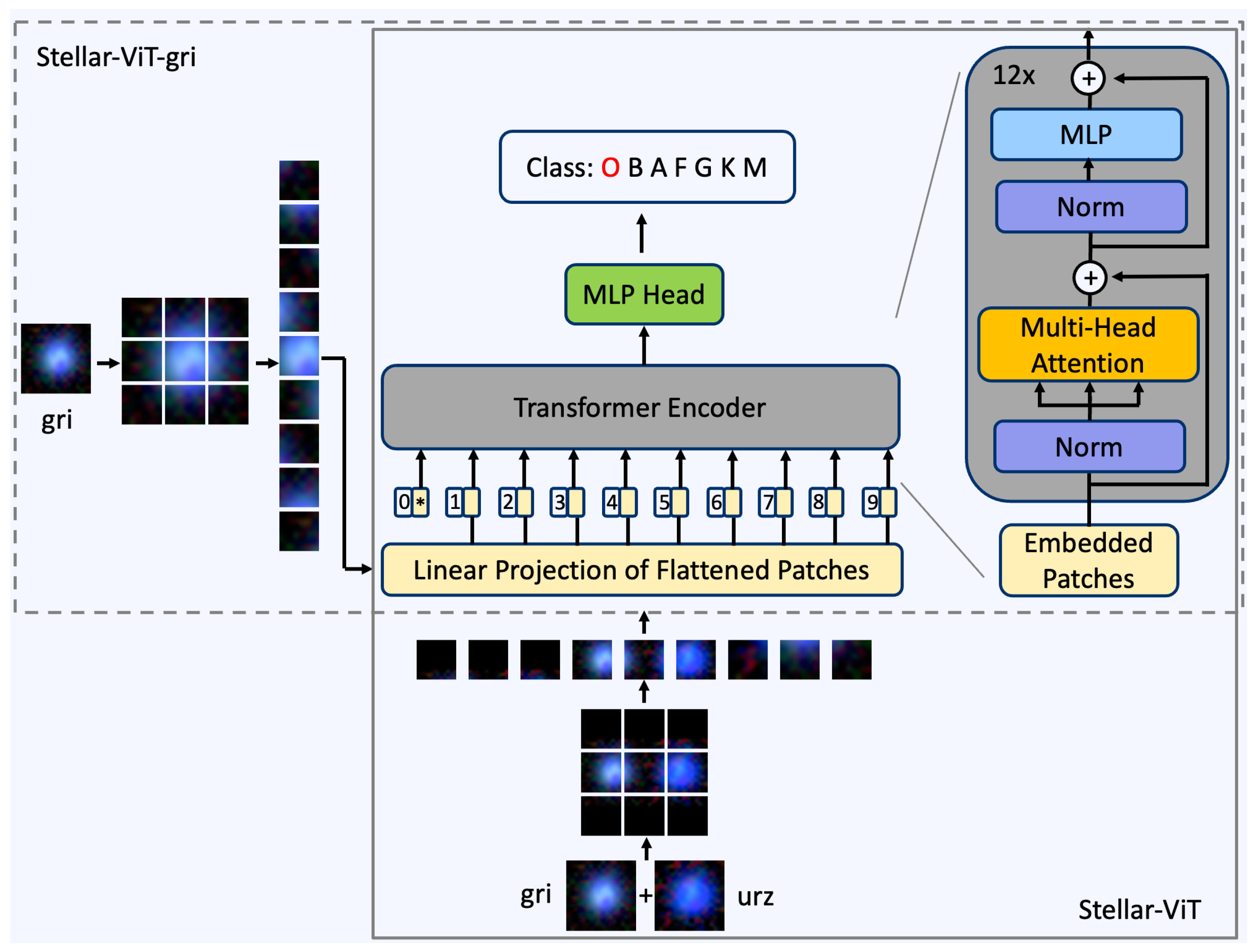
As shown in Figure 1, the architecture of ViT mainly consists of three parts: the input embedding layer, Transformer encoder, and output head. The original image is divided into equally sized patches. These patches are linearly projected into a high-dimensional space by the input embedding layer and supplemented with positional encoding to retain their spatial information. These processed patches are then ready to be fed into the Transformer encoder. The Transformer encoder is composed of multiple identical layers, each containing a multi-head self-attention (MHSA) module and a simple multi-layer perception (MLP) module. The MHSA allows the model to consider information from all other patches while processing each patch, thereby capturing the complex relationships and structures within the image. The output from the Transformer encoder is passed to an output head (usually one or more fully connected layers) for the final classification task.
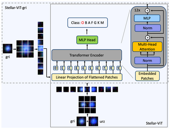
Figure 1.
ViT for stellar classification with image of gri or with image of combination of gri and urz. The red “O” indicates the model’s final prediction for the stellar type being examined. The details of the workflow of the network are given in Section 3.2.
The embedding layer consists of two parts: input embedding and position embedding. The input embedding linearly maps patches to a high-dimensional space, enabling the model to capture more complex features and patterns. In the high-dimensional space, the relative positions and distances between data points can more richly represent different semantic and syntactic relationships, thereby enhancing the model’s understanding of the input data. The position embedding maps pixel positions to specific embedding vectors, position information is encoded into the model to capture spatial relationships between pixels. Position embedding allows the model to accept inputs of arbitrary sizes without affecting the effectiveness of the position embedding.
The Transformer encoder is a core component of the ViT network, which achieves the mapping of variable-length vector sequences to sequences of the same length by stacking Transformer layers. Each Transformer layer consists of multi-head self-attention, multi-layer perceptron, and layer normalization modules. The MHSA mechanism divides the input sequence into multiple heads, computes various attention mechanisms in parallel, and then, concatenates the results to capture different information within the input sequence. Each head independently calculates attention weights, enabling the model to learn richer information representations. MLP enhances the model’s expressive power and performance by introducing a feedforward neural network that maps input sequences to a high-dimensional space, and then, undergoes a series of nonlinear transformations. The feedforward neural network lacks recurrent structures, thus avoiding the issues of gradient vanishing/exploding, making it easier to train and optimize. Layer normalization normalizes the input at each position to reduce internal covariate shift, making the model easier to train and converge. It can also improve the stability and convergence speed of the model, making the training process more stable and reliable. The outputs of the MHSA and MLP layers undergo residual connections and layer normalization.
The fundamental architecture of the Transformer relies solely on self-attention mechanisms, excluding recurrent and convolutional layers. The self-attention mechanism typically models the internal correlations within a sequence as follows:
The matrix representation of the input vector sequence is denoted as . According to Equation (1), is linearly projected to generate the query matrix , key matrix , and value matrix , where , , and are weight matrices.
Subsequently, the attention scores are computed by performing scaled matrix product operations on and , where is the number of dimensions of the attention query and key vector. This is followed by a softmax operation, and the resulting values are multiplied by to produce the output matrix.
A more common approach is to employ multi-head self-attention, mapping , , and h times to enable parallel computation to obtain Equation (2). The outputs are concatenated, and then, linearly projected. The fully connected feedforward network comprises fully connected layers activated by ReLU. Finally, a fully connected layer is applied for classification, with the output vector dimension matching the number of categories. During the training process, gradients are backpropagated to each individual encoder to update their parameters.
3.2. ViT for Stellar Classification
In the field of astronomy, the classification of stellar spectral types from images is an important and challenging task, involving the categorization of stellar spectral types from a large amount of astronomical observation data. Due to the difficulty in classifying stellar spectra from images and the limited number of stellar samples containing spectral data, traditional CNN models may encounter performance bottlenecks when processing such images. The Transformer model possesses powerful feature extraction capabilities and has begun to be utilized in the field of astronomy [23,24,25].
Considering the characteristics of stellar images and the performance of the ViT network in image classification tasks, the traditional CNN is replaced with the ViT network. By utilizing the properties of the Transformer module in the ViT network, the image is processed with self-attention mechanism to capture the image features. In the model design, it is necessary to take into account the characteristics of stellar images, such as the 5 different bands of stellar images, and convert them into learnable inputs for the ViT network (Figure 1).
As show in Figure 1, the process of stellar-ViT is as follows:
- The image is resized from 64 × 64 to 224 × 224.
- The image is then divided into 9 patches and transformed into patch embedding vectors through a linear projection layer.
- The patch embedding vectors are added to the position embedding vectors to obtain new embedding vectors, which serve as the input for the Transformer encoder.
- The Transformer encoder processes the embedding vectors based on self-attention, including steps such as normalization (Norm), multi-head attention, and multi-layer perceptron (MLP), to produce output embedding vectors.
- The output embedding vectors are fed into a classification head (MLP head) to obtain the predicted probabilities for each category of the sample.
3.3. Training Strategy for ViT
We employed a transfer learning strategy by initializing the Vision Transformer (ViT) with pre-trained weights from ImageNet, followed by fine-tuning on the stellar image classification data. ImageNet, which is presently the largest database for natural image recognition worldwide, comprises over 14 million images and 20,000 categories3 [26], and is commonly used for pre-training in transfer learning [27]. Image augmentation is performed by randomly rotating the images with a probability of 50% within the range of 0–30 degrees. In contrast to SCNet, we use the ordinary cross-entropy loss function instead of the weighted cross-entropy loss function. The Adam optimizer [28] is employed with a learning rate of , a batch size of 64, and a total of 50 training epochs. Additionally, a combination of warm-up and cosine annealing algorithms is employed to update the learning rate [29].
In this study, the training and test codes were based on Python 3.8.0 (Creator: Python Software Foundation, Location: Beaverton, OR, USA) and PyTorch 1.13.1 (Creator: Facebook, Inc., Location: Menlo Park, CA, USA). The training process was terminated within 20,000 iteration. We ran it on a graphics workstation with an Ubuntu 18.04.1 LTS OS, an Intel(R) Xeon(R) Platinum 8160 CPU, 256 GB RAM and an 24 GB NVIDIA GeForce RTX 3090 GPU. The corresponding versions of NVIDIA CUDA (Creator: NVIDIA Corporation, Location: Santa Clara, CA, USA) and cuDNN (Creator: NVIDIA Corporation, Location: Santa Clara, CA, USA) are 11.6 and 8.3.2, respectively.
4. Results and Analysis
4.1. Evaluation Metrics
In order to explore the classification performance of the model, we use accuracy to evaluate the overall performance of the model, and use F1 score to measure the model’s ability to predict different classes.
where is the number of total samples; (true positive) is the number of sources predicted to be the k-th class that actually are the class; (false positive) is the number of sources predicted to be the k-th class that actually are not the k-th class; and (false negative) is the number of sources predicted to not be the k-th class when actually they are the k-th class. Accuracy is the ratio of correctly predicted samples to the total samples, reflecting the model’s classification ability for the entire sample set. The precision of the k-th class, , is the ratio of to the total number of samples predicted to be the k-th class, which reflects the correctness of the model’s prediction result of the k-th class. The recall of the k-th class, , is the ratio of to the total number of samples of the k-th class, which reflects the ability of the model to find positive samples of the k-th class. The F1 score of the k-th class, , is the harmonic mean of and , with a larger value indicating better classification performance of the model for that category. The F1 score, as well as the precision and recall, are calculated separately for each class.
4.2. Comparison of Classification Performance
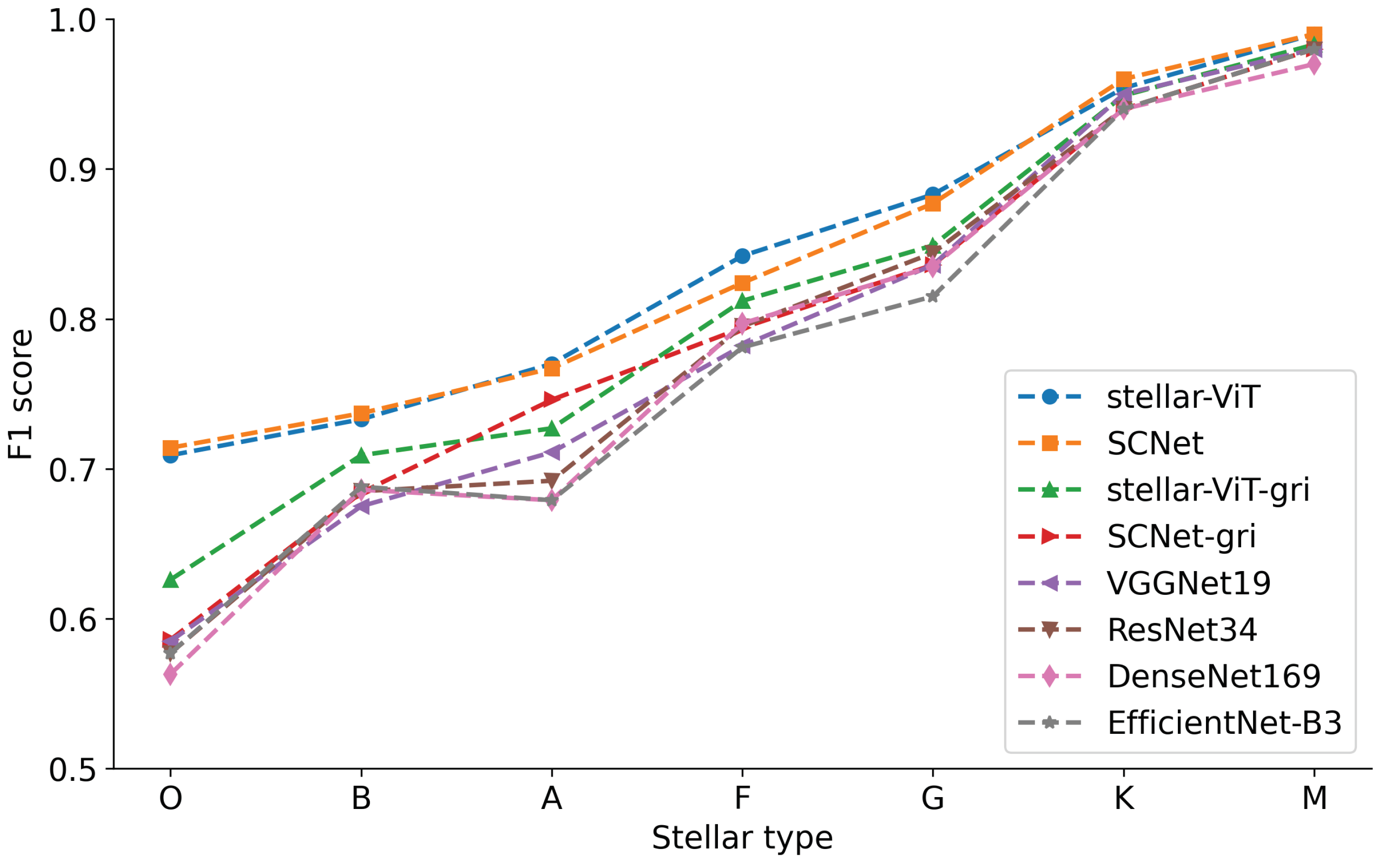
In the classification task based on photometric images, typically only RGB images converted from the gri band are used (e.g., [6,7,8,30,31]). For the classification task of RGB images in the gri band, we constructed a network (stellar-ViT-gri) for processing individual RGB images, with its network architecture shown in Figure 1. We compared it with several typical classification convolutional neural networks, including VGGNet19 [32], ResNet34 [33], DenseNet169 [34], EfficientNet-B3 [35], and SCNet-gri. All networks were trained on the same train set and evaluated on the same test set. Table 1 shows the performance of the best training models of each network in terms of F1 score and accuracy on the test set. From Table 1, it can be observed that the classification accuracy of stellar-ViT-gri is higher than the other five networks. The F1 scores for the majority of star types are also higher than the other five networks, except for type B, which is slightly lower than SCNet-gri by 0.015. Particularly for type O stars, the F1 score of stellar-ViT-gri reaches 0.626, making it the only classification model relying solely on gri data to exceed 0.6. This is quite similar to SCNet-gri, slightly higher by 0.04. The results indicate that stellar-ViT-gri performs better when classifying stars based solely on RGB images synthesized from the gri band.

Table 1.
Results for accuracy and F1 scores of the seven classification networks against the test set. The bold entries in the table highlight the best results using gri + urz images in each column and the underlined entries highlight the best results using only gri images in each column.
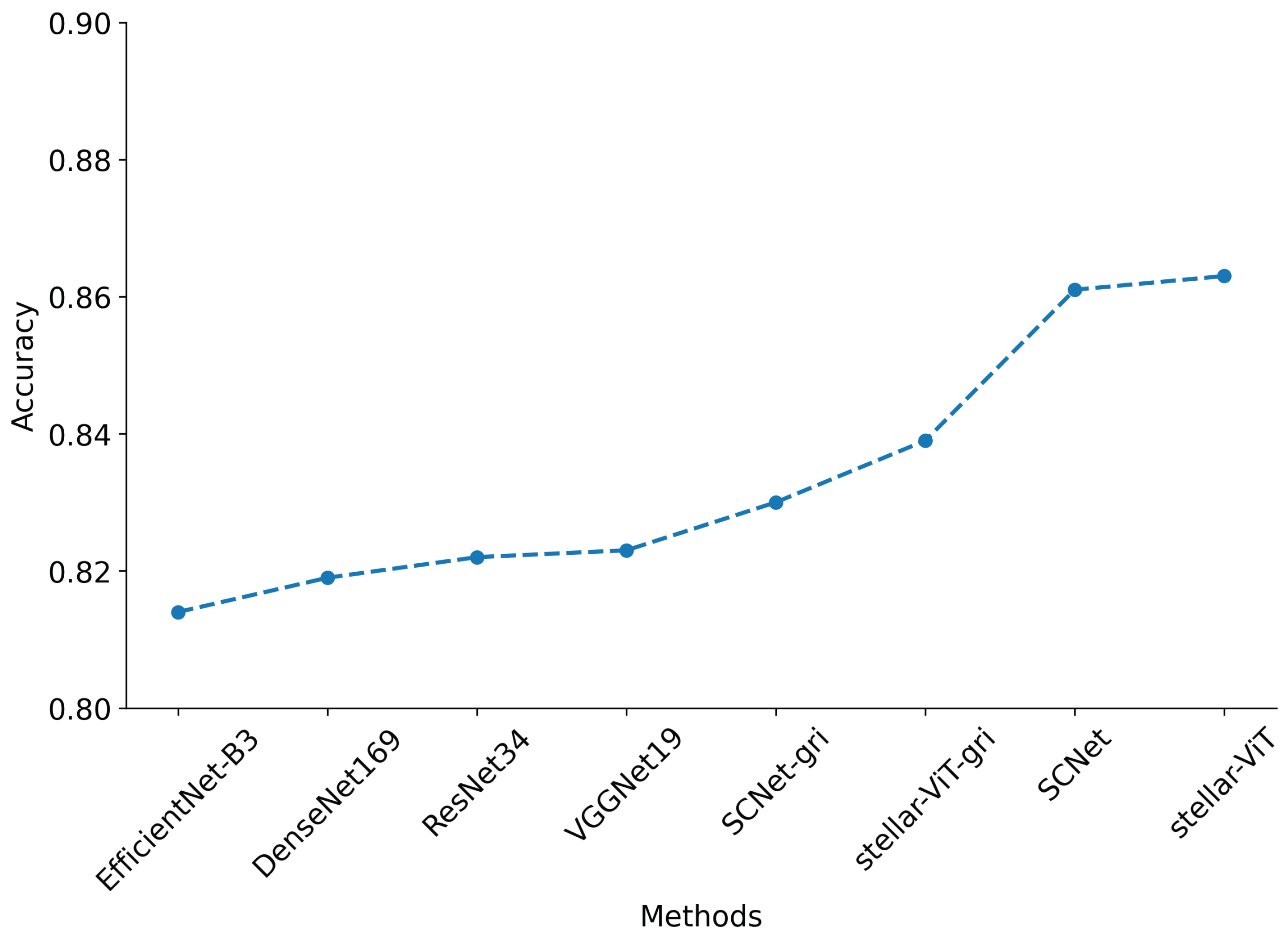
The SDSS photometric images consist of five bands: g, r, i, u, and z. RGB images synthesized by the stellar-ViT-gri using the g, r, and i bands does not utilize all the information available. To incorporate the information from the u and z bands, one approach is to synthesize RGB images using the u, r, and z bands, and input them into a convolutional neural network separately from the RGB images synthesized using the g, r, and i bands. These two sets of features are then fused through self-attention modules [15]. To fully leverage the powerful performance of self-attention mechanisms, we concatenate the two synthesized images and feed them into the stellar-ViT model constructed based on self-attention modules. The structure of stellar-ViT is illustrated in Figure 1, where the RGB input images of the gri bands and urz bands are concatenated into a new input image. By utilizing the long-range correlations of the Transformer self-attention module, the information from the uz bands is fused with the information from the gri bands. The performance metrics recorded in Table 1 demonstrate that stellar-ViT exhibits optimal accuracy. Compared to stellar-ViT-gri, stellar-ViT shows a significant improvement in classification performance. The overall classification accuracy increases from 0.839 to 0.863, as shown in Figure 2 and Table 1. The improvement is most pronounced for O-type stars, with the F1 score increasing from 0.626 to 0.709, as shown in Figure 3 and Table 1. The F1 score increases towards M-type stars, as shown in Figure 3, possibly due to the shift in stellar radiation from ultraviolet to visible light as temperature decreases, thereby covering more SDSS observation bands. The enhanced classification performance indicates that the u and z bands provide more useful information for stellar classification, and the effective fusion of this information is achieved through the long-range correlations of the Transformer self-attention mechanism.

Figure 2.
Results for accuracy of the 8 classification networks against the test set.
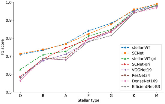
Figure 3.
Results for F1 score of the 8 classification networks against the test set.
4.3. Performance on Training Datasets of Varied Sizes
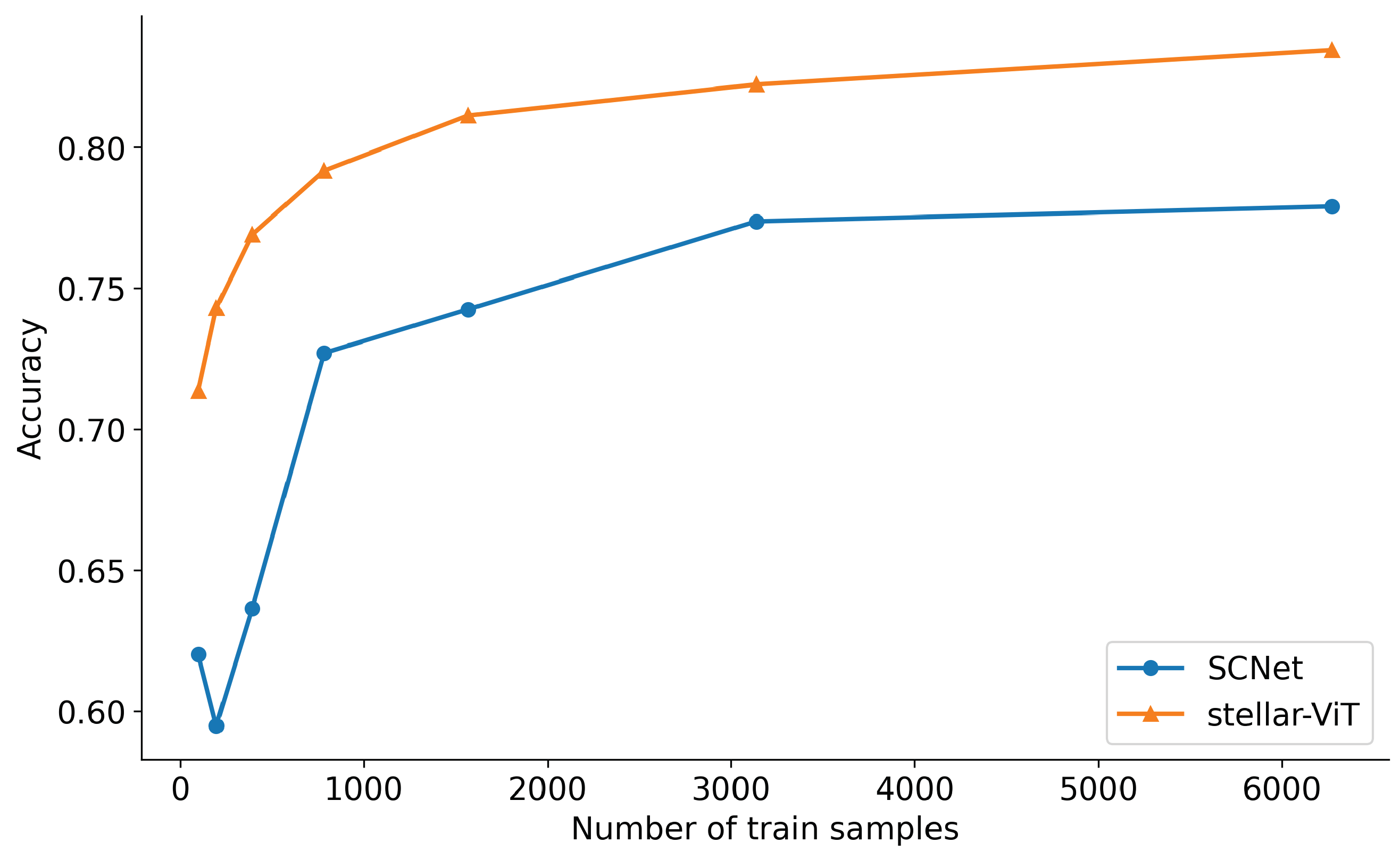
For the stellar-ViT model, we constructed different sizes of training sets containing 98, 196, 392, 784, 1568, 3136, and 6272 samples. For each group, a corresponding number of training samples was randomly selected to conduct 10 experiments, the average accuracy was calculated, and the impact of the training data size on the stellar classification performance was tested (see Figure 4). By employing this method, the potential impact of the data imbalance in the training set can be alleviated. For SCNet, the accuracies are as follows: 0.62, 0.595, 0.636, 0.727, 0.743, 0.774, and 0.779. For stellar-ViT, the accuracies are 0.714, 0.743, 0.769, 0.792, 0.811, 0.822, and 0.834. When the training dataset contains 1568 or more samples, the average accuracy of stellar-ViT is greater than 0.8. Most samples in the test set are correctly classified. Even when the training dataset size is reduced to 392 samples, stellar-ViT maintains a relatively high classification accuracy (>0.76). With only 98 samples, the classification accuracy noticeably decreases (approximately 0.7). When the number of samples in the training set is small, the classification accuracy improves as the training data size increases. As the training set size increases from 98 to 784, the accuracy rises from 0.7 to nearly 0.8. We conducted small-sample experiments on SCNet with the same configuration. The results indicate that, under the same number of samples, the accuracy of the stellar-ViT model is significantly higher than that of the SCNet model; especially, showing an increase of 0.15 in accuracy when the sample size is very small (192).
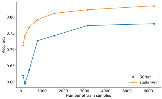
Figure 4.
The variation in classification accuracy across seven different-sized datasets.
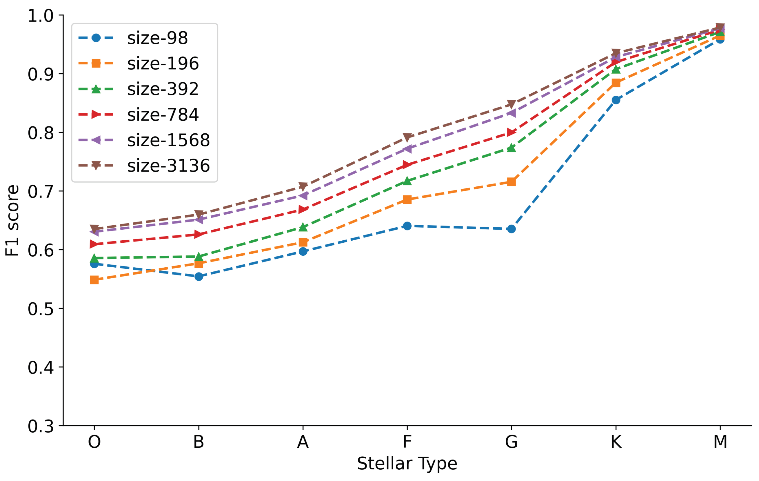
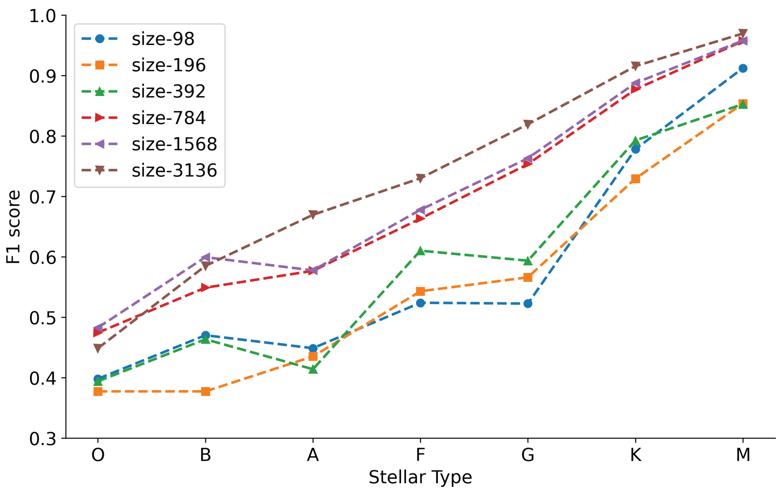
After comparing the performance of stellar-ViT on different sizes (98, 196, 392, 784, 1568, 3136, 6272) of datasets in predicting various types of stars on the same test set (Figure 5), we observe that, under the condition of equal sample sizes for each category in the training set, the size of the training dataset has little impact on the classification performance of M-type stars. As the training dataset size increases, the classification F1 scores of B-type, A-type, F-type, G-type, and K-type stars gradually improve, with the F1 score of G-type stars showing the fastest improvement. The impact of changes in training set size on the performance of the SCNet model in classifying O-type and M-type stars is relatively small (see Figure 6). The influence on B, F, and K types is minimal, while it is significant for A and G types. When the training set sample size decreases from 784 to 392, there is a noticeable sharp decline in the F1 scores for all seven types of stars, indicating that the SCNet model is sensitive to small sample sizes.

Figure 5.
Variation in F1 score of stellar-ViT trained on seven different-sized training sets across seven classes of stars.
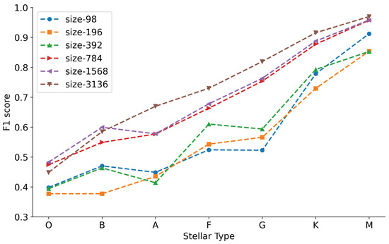
Figure 6.
Variation in F1 score of SCNet trained on seven different-sized training sets across seven classes of stars.
4.4. Discussion
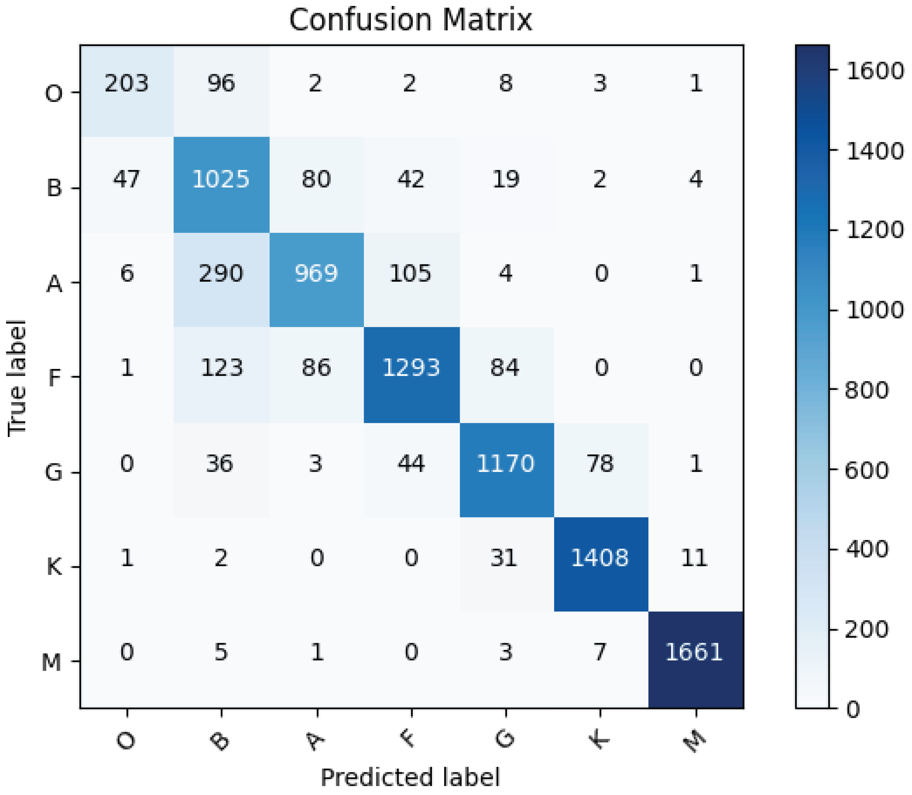
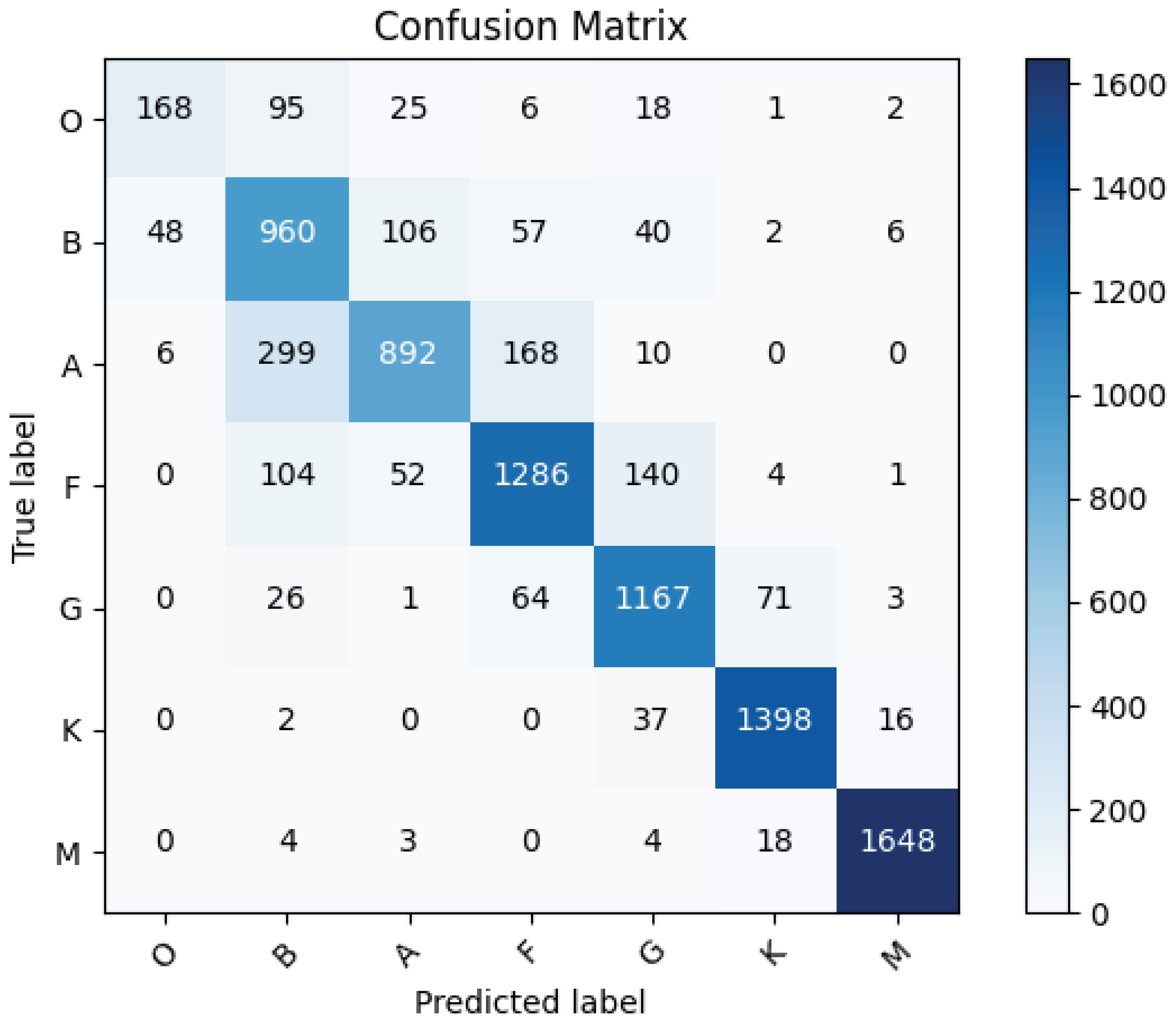
Figure 7 shows the confusion matrix of stellar-ViT on the test set. The columns represent the predicted categories, with the total in each column indicating the number of predictions for that category. The rows represent the true categories, with the total in each row indicating the actual number for that category. The main diagonal represents the correct predictions of the model, while non-zero values outside the diagonal indicate incorrect predictions. Most predictions in the confusion matrix fall along the main diagonal, indicating the model’s good classification ability. The misclassified samples are mainly distributed among adjacent categories. For example, out of 395 misclassified type A stars, 290 were misclassified as type B and 105 as type F. This suggests that distinguishing between adjacent subcategories remains a major challenge in stellar spectral type classification. Adjacent spectral types often exhibit overlapping characteristics in their spectra. This overlap is due to the continuous nature of stellar temperatures and the gradual changes in stellar atmospheres. As a result, the photometric images that are used to classify stars can appear very similar in adjacent types, making it challenging to assign a definitive classification. Comparing the confusion matrices obtained from the predictions of stellar-ViT-gri on the test set (Figure 8) and stellar-ViT (Figure 7), we observe that in comparison to stellar-ViT-gri, the number of misclassifications into adjacent classes in the stellar-ViT classification results remains relatively constant, while the number of misclassifications into classes with lower temperature decreases, as shown in the bottom left corners of Figure 7 and Figure 8.
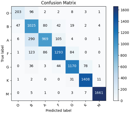
Figure 7.
Confusion matrix resulting from predictions of stellar-ViT on the test set.

Figure 8.
Confusion matrix resulting from predictions of stellar-ViT-gri on the test set.
This indicates that merging two channels for prediction can to some extent reduce the occurrence of distant misclassifications. For type B stars, stellar-ViT cannot reduce the number of samples misclassified as type O, but it can significantly reduce the number misclassified as type A. For type F stars, stellar-ViT can notably reduce the number misclassified as type G. For B-, A-, and F-type stars, incorporating u and z data into the stellar-ViT model can significantly reduce the likelihood of misclassifying them as neighboring cooler types.
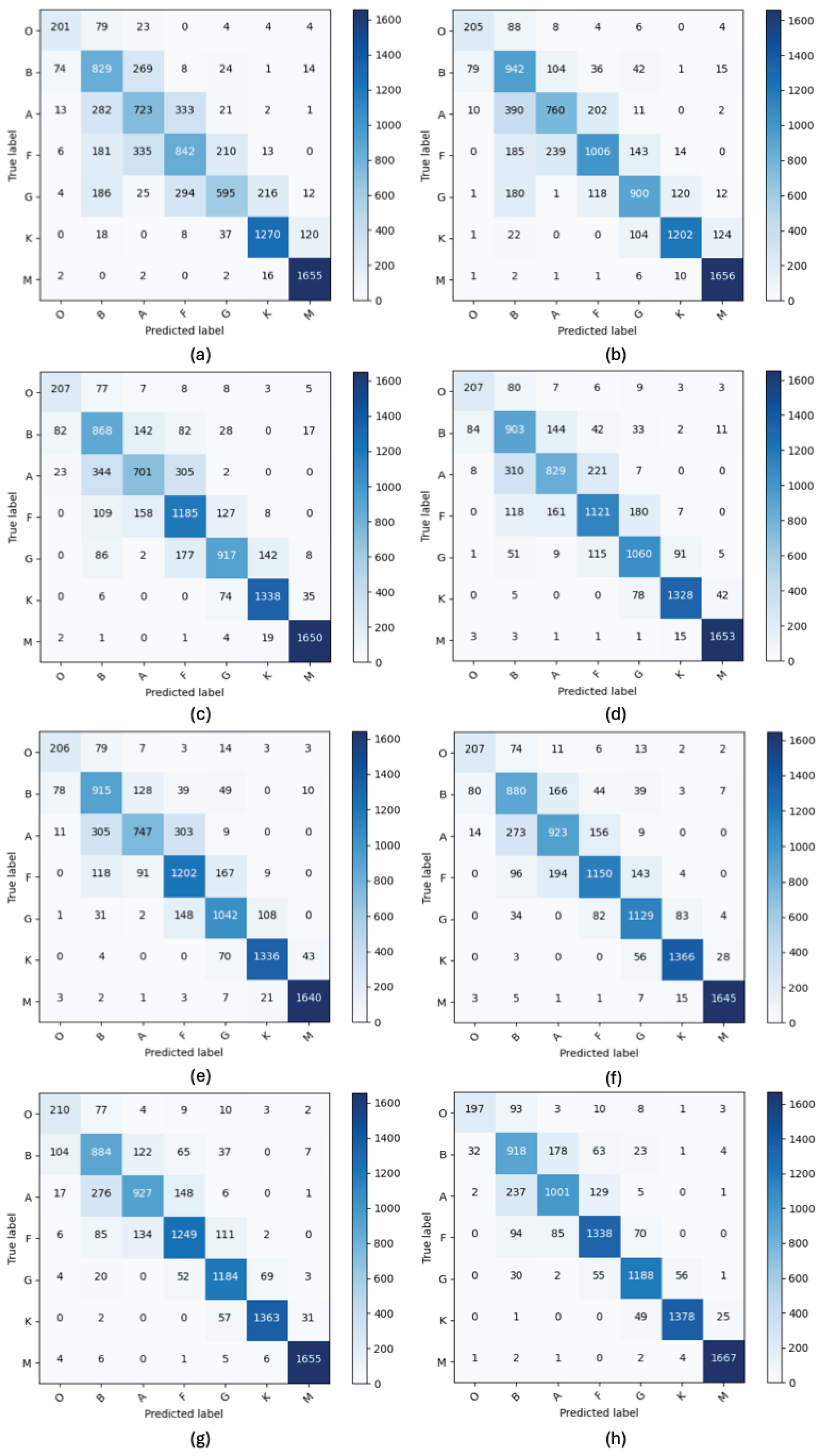
When comparing the confusion matrices obtained from predicting on the same test set after training on different sizes (98, 196, 392, 784, 1568, 3136, 6272, 31327) of the stellar-ViT dataset (Figure 9), it is observed that, under the condition of equal sample sizes for each class in the training set, the size of the training dataset has little impact on the classification performance of O-type and M-type stars. The possible reason may be that the radiation from O-type stars is primarily concentrated in the ultraviolet region, and the photometric images we use are unable to capture most of the radiation energy emitted by O-type stars. This affects the accuracy of classification based on color and brightness, and increasing the sample size is insufficient to address this issue. In contrast, M-type stars have a lower temperature compared to other stellar categories, resulting in more pronounced differences in luminosity in photometric images, which allows for good classification results even with a smaller sample size. However, continuing to increase the sample size yields limited improvement. As the training dataset size increases, there is no significant improvement in the classification accuracy of B-type stars, while the classification accuracy of A-type, F-type, G-type, and K-type stars gradually improves. As for the misclassification issues encountered with B-, A-, F-, and G-type stars, the likely cause is the spectral overlap between these categories. This overlap means that luminosity images might not capture the subtle features necessary for accurate differentiation, leading to poorer classification outcomes.
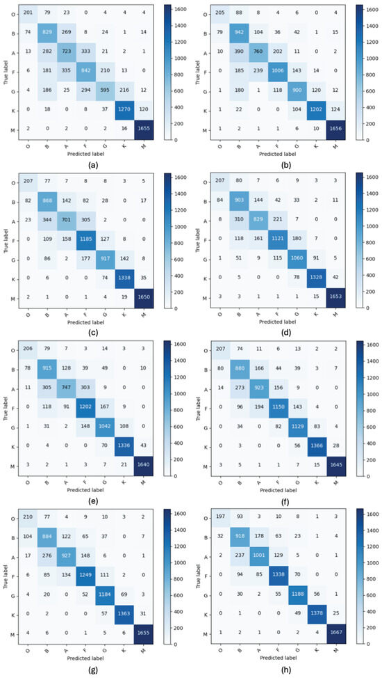
Figure 9.
Confusion matrices resulting from predictions on the test set by stellar-ViT trained on train sets of various sizes: (a) 98, (b) 196, (c) 392, (d) 784, (e) 1568, (f) 3136, (g) 6272, and (h) 31,327.
5. Conclusions
In this study, we propose a novel stellar classification network, stellar-ViT, based on the Transformer architecture, aiming to classify stars solely relying on photometric images. We utilize RGB images synthesized from the photometric data of SDSS for training and testing the model, encompassing seven main categories: O, B, A, F, G, K, and M. Our model, stellar-ViT-gri, demonstrates superior performance when processing RGB images from the gri bands, outperforming classical CNN networks such as VGGNet19, ResNet34, DenseNet169, and EfficientNet-B3, as well as SCNet-gri. Furthermore, our stellar-ViT model excels in handling RGB images synthesized from the gri and urz bands, achieving an overall accuracy of 0.863, surpassing classical CNN networks and the current state-of-the-art stellar classification network, SCNet.
Our approach is simple and efficient, concatenating two RGB images composed of five-band data for stellar classification. Furthermore, our data augmentation strategy only involves random rotation, eliminating the need for other types of enhancements like grayscale stretching, used in SCNet, or weighted cross-entropy to balance sample quantities. These characteristics not only simplify the training process but also demonstrate the feasibility of using photometric images and Transformer for stellar classification, particularly maintaining good performance in small sample scenarios and effectively reducing the likelihood of misclassifying samples into higher-temperature adjacent subclasses.
Through in-depth analysis, our research not only showcases the outstanding performance of the stellar-ViT model in stellar spectral type classification tasks but also highlights the high accuracy classification ability of our model, especially the variant stellar-ViT-gri when processing gri band RGB images. Compared to several typical convolutional networks and the latest stellar image classification networks, our model outperforms all comparative models on the test set, particularly excelling in the classification of O-type stars, where the F1 score of the stellar-ViT-gri model reaches 0.626, the only model surpassing an F1 score of 0.6, outperforming the state-of-the-art SCNet-gri model by 0.04. The impact of additional band information on model performance is also emphasized. By combining RGB images from the gri band with those from the urz band and utilizing the self-attention mechanism of the Transformer model, our stellar-ViT model effectively integrates this additional information, significantly enhancing classification performance. Specifically, the overall classification accuracy improves from 0.839 to 0.863, and the F1 score for O-type stars increases from 0.626 to 0.709, underscoring the importance of u and z band information in enhancing stellar classification performance.
We investigate the influence of training dataset size on model performance. The results indicate that when the training dataset contains 1568 or more samples, the average accuracy of the stellar-ViT model exceeds 0.8, enabling correct classification of most stars. Even with a reduced training sample size of 392, the model maintains a high accuracy (>0.76). This finding suggests that our model exhibits good robustness to training dataset size, particularly in scenarios with fewer samples.
Through the analysis of confusion matrices, we further confirm the model’s classification ability, particularly in distinguishing adjacent subclasses. Compared to the stellar-ViT-gri model using only the gri band, the stellar-ViT model incorporating u and z band data performs better in reducing misclassifications, especially in decreasing the likelihood of misclassifying stars as adjacent higher-temperature types.
In conclusion, our research not only demonstrates the exceptional performance of the stellar-ViT model in stellar spectral type classification tasks but also underscores the impact of additional band information and training dataset size on model performance, providing valuable insights for future research in this field.
In future work, we plan to further enhance the model’s classification accuracy. Considering that Transformer networks are well-suited for unsupervised learning and the SDSS data contains a substantial amount of unlabeled stellar data, we will explore utilizing this unlabeled data for unsupervised learning with Transformers to further improve the classification accuracy of the stellar-ViT model. Additionally, we believe the stellar-ViT model has the potential to be extended to classifying other types of astronomical survey data, offering broader applications in the field of astronomy.
Author Contributions
Y.Y. conceived of the study, and performed the algorithm design and coding, dataset preparation, data analysis, and manuscript writing. X.L. participated in manuscript revision. All authors have read and agreed to the published version of the manuscript.
Funding
This work is supported by the National Science Foundation of China [Grant No. 32300381] and the Innovation Project of Beijing Academy of Science and Technology (24CD013). The funders had no role in the design of the study, in the collection, analysis, and interpretation of the data, or in the writing of the manuscript.
Data Availability Statement
No new data were created or anlyzed in this study. Data sharing is not applicable to this article.
Acknowledgments
During the preparation of this work the authors used the GPT-4 model in order to improve the readability and language of our paper. After using this tool, the authors reviewed and edited the content as needed.
Conflicts of Interest
The authors declare no conflicts of interest.
Notes
| 1 | The latest release is DR 18, for the fifth phase of SDSS. |
| 2 | http://skyserver.sdss.org/dr16/en/help/docs/api.aspx#imgcutout, accessed on 1 September 2023. |
| 3 | Accessed on 11 April 2023 via http://www.image-net.org. |
References
- Sharma, K.; Kembhavi, A.; Kembhavi, A.; Sivarani, T.; Abraham, S.; Vaghmare, K. Application of Convolutional Neural Networks for Stellar Spectral Classification. Mon. Not. R. Astron. Soc. 2020, 491, 2280–2300. [Google Scholar] [CrossRef]
- Garrison, R.F.; MacConnel, D.J.; Straizys, V.; Keenan, P.C.; Jaschek, C.; Slettebak, A. Stellar Classification. In Reports on Astronomy; Wayman, P.A., Ed.; Springer: Dordrecht, The Netherlands, 1982; pp. 621–632. [Google Scholar] [CrossRef]
- Abdurro’uf; Accetta, K.; Aerts, C.; Aguirre, V.S.; Ahumada, R.; Ajgaonkar, N.; Ak, N.F.; Alam, S.; Prieto, C.A.; Almeida, A.; et al. The Seventeenth Data Release of the Sloan Digital Sky Surveys: Complete Release of MaNGA, MaStar, and APOGEE-2 Data. ApJS 2022, 259, 35. [Google Scholar] [CrossRef]
- Brown, T.M.; Latham, D.W.; Everett, M.E.; Esquerdo, G.A. Kepler Input Catalog: Photometric Calibration and Stellar Classification. AJ 2011, 142, 112. [Google Scholar] [CrossRef]
- Kim, E.J.; Brunner, R.J. Star–Galaxy Classification Using Deep Convolutional Neural Networks. Mon. Not. R. Astron. Soc. 2017, 464, 4463–4475. [Google Scholar] [CrossRef]
- Zhu, X.P.; Dai, J.M.; Bian, C.J.; Chen, Y.; Chen, S.; Hu, C. Galaxy Morphology Classification with Deep Convolutional Neural Networks. Astrophys. Space Sci. 2019, 364, 55. [Google Scholar] [CrossRef]
- Osborn, H.P.; Ansdell, M.; Ioannou, Y.; Sasdelli, M.; Angerhausen, D.; Caldwell, D.; Jenkins, J.M.; Räissi, C.; Smith, J.C. Rapid Classification of TESS Planet Candidates with Convolutional Neural Networks. A&A 2020, 633, A53. [Google Scholar] [CrossRef]
- Lu, Y.K.; Qiu, B.; Luo, A.L.; Kong, X.; Jiang, X.; Guo, X.; Wang, L. Using CFSVM Model to Classify Stars from Three-Colour Images. Mon. Not. R. Astron. Soc. 2021, 507, 4095–4101. [Google Scholar] [CrossRef]
- Farias, H.; Ortiz, D.; Damke, G.; Jaque Arancibia, M.; Solar, M. Mask Galaxy: Morphological Segmentation of Galaxies. Astron. Comput. 2020, 33, 100420. [Google Scholar] [CrossRef]
- Jia, P.; Liu, Q.; Sun, Y. Detection and Classification of Astronomical Targets with Deep Neural Networks in Wide-field Small Aperture Telescopes. AJ 2020, 159, 212. [Google Scholar] [CrossRef]
- He, Z.; Qiu, B.; Luo, A.L.; Shi, J.; Kong, X.; Jiang, X. Deep Learning Applications Based on SDSS Photometric Data: Detection and Classification of Sources. Mon. Not. R. Astron. Soc. 2021, 508, 2039–2052. [Google Scholar] [CrossRef]
- D’Isanto, A.; Polsterer, K.L. Photometric Redshift Estimation via Deep Learning - Generalized and Pre-Classification-Less, Image Based, Fully Probabilistic Redshifts. A&A 2018, 609, A111. [Google Scholar] [CrossRef]
- Wu, J.F.; Boada, S. Using Convolutional Neural Networks to Predict Galaxy Metallicity from Three-Colour Images. Mon. Not. R. Astron. Soc. 2019, 484, 4683–4694. [Google Scholar] [CrossRef]
- Schuldt, S.; Suyu, S.H.; Cañameras, R.; Taubenberger, S.; Meinhardt, T.; Leal-Taixé, L.; Hsieh, B.C. Photometric Redshift Estimation with a Convolutional Neural Network: NetZ. A&A 2021, 651, A55. [Google Scholar] [CrossRef]
- Shi, J.H.; Qiu, B.; Luo, A.L.; He, Z.D.; Kong, X.; Jiang, X. Stellar Classification with Convolutional Neural Networks and Photometric Images: A New Catalogue of 50 Million SDSS Stars without Spectra. Mon. Not. R. Astron. Soc. 2023, 520, 2269–2280. [Google Scholar] [CrossRef]
- Vaswani, A.; Shazeer, N.; Parmar, N.; Uszkoreit, J.; Jones, L.; Gomez, A.N.; Kaiser, L.; Polosukhin, I. Attention Is All You Need. In Proceedings of the Advances in Neural Information Processing Systems; Curran Associates, Inc.: New York, NY, USA, 2017; Volume 30. [Google Scholar]
- Dosovitskiy, A.; Beyer, L.; Kolesnikov, A.; Weissenborn, D.; Zhai, X.; Unterthiner, T.; Dehghani, M.; Minderer, M.; Heigold, G.; Gelly, S.; et al. An Image Is Worth 16 × 16 Words: Transformers for Image Recognition at Scale. arXiv 2021, arXiv:2010.11929. [Google Scholar]
- Chen, C.F.R.; Fan, Q.; Panda, R. CrossViT: Cross-Attention Multi-Scale Vision Transformer for Image Classification. In Proceedings of the IEEE/CVF International Conference on Computer Vision, Montreal, BC, Canada, 11–17 October 2021; pp. 357–366. [Google Scholar]
- Hwang, S.Y.; Sabiu, C.G.; Park, I.; Hong, S.E. The Universe Is Worth 643 Pixels: Convolution Neural Network and Vision Transformers for Cosmology. J. Cosmol. Astropart. Phys. 2023, 2023, 75. [Google Scholar] [CrossRef]
- Cao, J.; Xu, T.; Deng, Y.; Deng, L.; Yang, M.; Liu, Z.; Zhou, W. Galaxy Morphology Classification Based on Convolutional Vision Transformer (CvT). Astron. Astrophys. 2024, 683, A42. [Google Scholar] [CrossRef]
- Lupton, R.; Blanton, M.R.; Fekete, G.; Hogg, D.W.; O’Mullane, W.; Szalay, A.; Wherry, N. Preparing Red-Green-Blue Images from CCD Data. Publ. Astron. Soc. Pac. 2004, 116, 133–137. [Google Scholar] [CrossRef]
- Bengio, Y.; Courville, A.; Vincent, P. Representation Learning: A Review and New Perspectives. IEEE Trans. Pattern Anal. Mach. Intell. 2013, 35, 1798–1828. [Google Scholar] [CrossRef]
- Lin, J.Y.Y.; Liao, S.M.; Huang, H.J.; Kuo, W.T.; Ou, O.H.M. Galaxy Morphological Classification with Efficient Vision Transformer. arXiv 2022, arXiv:2110.01024. [Google Scholar]
- Donoso-Oliva, C.; Becker, I.; Protopapas, P.; Cabrera-Vives, G.; Vishnu, M.; Vardhan, H. ASTROMER—A Transformer-Based Embedding for the Representation of Light Curves. A&A 2023, 670, A54. [Google Scholar] [CrossRef]
- Pan, J.S.; Ting, Y.S.; Yu, J. Astroconformer: The Prospects of Analyzing Stellar Light Curves with Transformer-Based Deep Learning Models. Mon. Not. R. Astron. Soc. 2024, 528, stae068. [Google Scholar] [CrossRef]
- Deng, J.; Dong, W.; Socher, R.; Li, L.J.; Li, K.; Fei-Fei, L. ImageNet: A Large-Scale Hierarchical Image Database. In Proceedings of the 2009 IEEE Conference on Computer Vision and Pattern Recognition, Miami, FL, USA, 20–25 June 2009; pp. 248–255. [Google Scholar] [CrossRef]
- He, K.; Girshick, R.; Dollar, P. Rethinking ImageNet Pre-Training. In Proceedings of the IEEE/CVF International Conference on Computer Vision, Seoul, Republic of Korea, 27 October–2 November 2019; pp. 4918–4927. [Google Scholar]
- Kingma, D.P.; Ba, J.L. Adam: A Method for Stochastic Optimization. In Proceedings of the 3rd International Conference on Learning Representations, ICLR 2015—Conference Track Proceedings, San Diego, CA, USA, 7–9 May 2015. [Google Scholar]
- Loshchilov, I.; Hutter, F. SGDR: Stochastic Gradient Descent with Warm Restarts. In Proceedings of the 5th International Conference on Learning Representations, ICLR 2017, Toulon, France, 24–26 April 2017; Conference Track Proceedings. OpenReview.net: Boston, MA, USA, 2017. [Google Scholar]
- Dieleman, S.; Willett, K.W.; Dambre, J. Rotation-Invariant Convolutional Neural Networks for Galaxy Morphology Prediction. Mon. Not. R. Astron. Soc. 2015, 450, 1441–1459. [Google Scholar] [CrossRef]
- Khramtsov, V.; Dobrycheva, D.V.; Vasylenko, M.Y.; Akhmetov, V.S. Deep Learning for Morphological Classification of Galaxies from SDSS. Odessa Astron. Publ. 2019, 32, 21–23. [Google Scholar] [CrossRef]
- Simonyan, K.; Zisserman, A. Very Deep Convolutional Networks for Large-Scale Image Recognition. arXiv 2015, arXiv:1409.1556. [Google Scholar]
- He, K.; Zhang, X.; Ren, S.; Sun, J. Deep Residual Learning for Image Recognition. In Proceedings of the 2016 IEEE Conference on Computer Vision and Pattern Recognition (CVPR), Las Vegas, NV, USA, 27–30 June 2016; pp. 770–778. [Google Scholar] [CrossRef]
- Huang, G.; Liu, Z.; Van Der Maaten, L.; Weinberger, K.Q. Densely Connected Convolutional Networks. In Proceedings of the 2017 IEEE Conference on Computer Vision and Pattern Recognition (CVPR), Honolulu, HI, USA, 21–26 July 2017; pp. 2261–2269. [Google Scholar] [CrossRef]
- Tan, M.; Le, Q. EfficientNet: Rethinking Model Scaling for Convolutional Neural Networks. In Proceedings of the 36th International Conference on Machine Learning, PMLR, Long Beach, CA, USA, 9–15 June 2019; pp. 6105–6114. [Google Scholar]
Disclaimer/Publisher’s Note: The statements, opinions and data contained in all publications are solely those of the individual author(s) and contributor(s) and not of MDPI and/or the editor(s). MDPI and/or the editor(s) disclaim responsibility for any injury to people or property resulting from any ideas, methods, instructions or products referred to in the content. |
© 2024 by the authors. Licensee MDPI, Basel, Switzerland. This article is an open access article distributed under the terms and conditions of the Creative Commons Attribution (CC BY) license (https://creativecommons.org/licenses/by/4.0/).

