1. Introduction
Quantum gravitational states of ultracold neutrons in the gravitational field of the Earth above a mirror have a long history [
1,
2,
3,
4,
5] and have been experimentally observed in several studies [
6,
7,
8,
9,
10,
11,
12,
13,
14,
15]. The experimental analysis of the spatial probability density distribution for these quantum gravitational states has been extensively studied. Such investigations typically involve measuring the free fall of ultracold neutrons onto a mirror, as reviewed in [
16,
17,
18,
19,
20,
21].
Furthermore, transitions between quantum gravitational states of ultracold neutrons, bouncing between two mirrors in the Earth’s gravitational field, have been experimentally examined in [
22,
23]. Theoretical calculations of wave functions and binding energies for quantum gravitational states of ultracold neutrons confined between two mirrors are reported in [
24] (see also [
25,
26]).
Recently, experimental data on the spatial distribution of ultracold neutrons in the Earth’s gravitational field above a mirror, obtained by Ichikawa et al. [
27], were interpreted as representing the spatial distribution of quantum gravitational states. In their study, the authors analyzed the vertical distribution of ultracold neutrons above a horizontal mirror, as projected onto a pixelated horizontal detector. This was achieved by scattering neutrons off a cylindrical mirror. The observed spatial modulation was interpreted as the spatial distribution of quantum gravitational states. To support this interpretation, the authors performed a theoretical analysis of the experimental data using the Wigner function formalism [
28,
29].
In this paper, we analyze the spatial distribution of quantum gravitational states of ultracold neutrons for the experimental setup employed by Ichikawa et al. [
27]. Specifically, we examine the distribution in terms of: (i) the spatial probability density [
30] and (ii) the spatial distribution of the Wigner function [
28,
29] of these states. However, our theoretical analysis indicates that the experimental data reported by Ichikawa et al. [
27] do not conclusively correspond to the spatial distribution of quantum gravitational states of ultracold neutrons.
2. Experimental Setup of Ichikawa’s Experiment on Spatial
Distribution of Quantum Gravitational States of Ultracold Neutrons
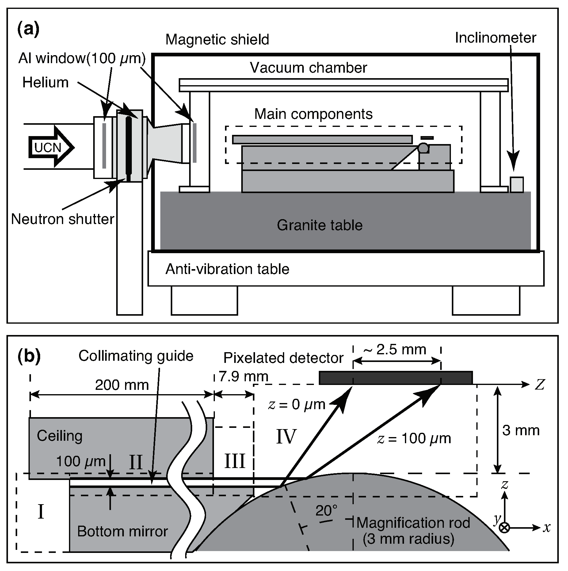
The experimental setup for measuring the spatial distribution of ultracold neutrons above a cylindrical mirror, shown in
Figure 1, is adapted from [
27].
According to [
27], ultracold neutrons moving in the
x-direction in spatial region II, with a length
between two parallel plane mirrors separated by a distance
, are prepared in a quantum gravitational state
. This state is a mixed state, expressed as
, where
are stationary pure quantum gravitational states of ultracold neutrons. Here,
represents the principal quantum number, and
corresponds to the time at which ultracold neutrons are injected into spatial region II. The phases
are random.
The equal population of quantum states arises from a thermal equilibrium and the small energy differences between states at ultracold temperatures, leading to a nearly uniform distribution of neutrons among the available states. The randomness of the phases is attributed to decoherence, the preparation process, and the quantum measurement process, all of which contribute to a lack of coherence between the phases of neutrons in different quantum states.
The time evolution of ultracold neutrons in spatial region II for is described by the wave function . Here, , where are real functions, and is the binding energy of ultracold neutrons in the -quantum gravitational state between the two mirrors.
The horizontal motion of ultracold neutrons can, in principle, be described by a plane wave , where and represent the momentum and energy of horizontal motion, respectively. This approximation is valid, as there are no significant external forces or potential gradients affecting the neutrons horizontally, allowing them to behave as free particles in that direction. The plane wave simplification effectively represents particles with constant momentum, aligning with the conditions of horizontal motion for ultracold neutrons. This description simplifies the analysis of neutron behavior, particularly in scattering and interference experiments.
The horizontal velocity
of ultracold neutrons follows a nearly Gaussian distribution centered at a mean value
with a standard deviation
[
27]. Thus, the wave function of ultracold neutrons in spatial region II is
, with
.
After traversing spatial region II, ultracold neutrons enter spatial region III, with a length
, bounded by a mirror below. In this region, the stationary pure quantum gravitational states are described by the wave functions
, where
is the binding energy, and
denotes the principal quantum number. The wave function of the mixed state
transforms into
, where
are random phases. The coefficients
are defined as:
At
, and the transition occurs between regions II and III. Integration is performed over
, as
vanishes outside this range. The differences in binding energies
do not vanish because
for any
n and
.
Finally, ultracold neutrons arrive at spatial region IV, where they move above a cylindrical glass rod acting as a mirror [
27]. The mechanism explaining the experimental results from Ichikawa et al. [
27] is as follows: neutrons with a momentum
and a de Broglie wavelength
scatter off the cylindrical mirror as classical particles. This scattering projects impact parameters
b onto the
Z-axis of the horizontal detector surface parallel to the
x-axis. Since the impact parameter
b is weighted by
, the specific spatial modulation observed along the
Z-axis matches the results reported by Ichikawa et al. [
27].
3. Impact Parameter of Scattering of Ultracold Neutrons as Classical
Particles by Cylindrical Mirror
Ultracold neutrons scatter off the cylindrical mirror with a momentum , corresponding to a wavelength . This wavelength is significantly smaller than the characteristic scale of gravitational quantum states. Therefore, ultracold neutrons interact with the cylindrical mirror as classical particles. The spatial distribution of ultracold neutrons along the Z-axis of the pixelated detector is determined by the relationship between the impact parameter b, the scattering angle , and the geometric parameters of the cylindrical mirror (R, ).
Figure 2 illustrates the scattering geometry for ultracold neutrons interacting with a rigid cylindrical mirror, as described in the experiment by Ichikawa et al. [
27]. The radius of the mirror is
, and the angle
.
Based on the geometry shown in
Figure 2, the impact parameter
b can be expressed as a function of the angle
and the azimuthal angle
as follows:
where
is related to the scattering angle
by
.
The azimuthal angle
and
are further related by:
Inverting these relationships,
can be expressed as follows:
Using these expressions, the impact parameter
b in terms of the scattering angle
becomes:
The maximal impact parameter
corresponds to the height of region II,
, which defines the minimal scattering angle:
The maximal scattering angle
is determined by the condition
, giving the following:
Thus, the endpoints of the interval
on the
Z-axis are shifted with respect to points
and
, which correspond to the maximal and minimal scattering angles, respectively. These shifts are calculated as follows:
Points
and
are the projections of
and
, respectively. As a result, the spatial distribution of ultracold neutrons can be observed along the
Z-axis in the following interval:
4. Projection of Ultracold Neutrons with Impact Parameter
onto -Axis of Pixelated Detector
As we have shown in
Section 3, ultracold neutrons, moving with an impact parameter
with a velocity
, are projected by a cylindrical mirror onto the
Z-axis of the pixelated detector. We may define such a projection as follows:
where
for
. Using the relations
we obtain
Z as a function of an impact parameter
b
At
we obtain
. Then, taking into account the values of the parameters of the experimental setup of Ichikawa’s experiment [
27], we may approximate the impact parameter
b by the expression
where
. At
, we obtain
. Thus, Equation (
4) allows to fit the maximal value of the impact parameter with an accuracy of about 1%. A derivative
is
Now, we are able to use the impact parameter
for the analysis of a spatial distribution of ultracold neutrons by a pixelated detector.
5. Spatial Distribution of Energy Levels of Quantum Gravitational
States of Ultracold Neutrons Between Two Mirrors
For the subsequent analysis of the experimental data by Ichikawa et al. [
27], it is necessary to determine the distribution of quantum gravitational states of ultracold neutrons within spatial region II. The energy levels of these states are defined by the roots of the following equation [
24]:
where
is the height of spatial region II, and
is a quantum scale associated with the quantum gravitational states of ultracold neutrons. Here,
g represents the gravitational acceleration. The roots
of Equation (
6) define the energy levels
, where
is the principal quantum number, and
.
The maximal number of quantum gravitational states
is determined by the condition
. Setting
and recognizing that
, we arrive at the equation. For
and using the asymptotic behavior of the Airy functions for
, Equation (
6) can be rewritten as follows:
the root of which is given by:
This defines the maximal number of the quantum gravitational states of ultracold neutrons within spatial region II.
The same result, along with the spatial distribution of quantum gravitational levels in region II, can be obtained using the quasi-classical approximation of quantum mechanics [
30]. In this approximation, the maximal number of quantum gravitational states of ultracold neutrons in the spatial region
is given by:
where
is the classical momentum of ultracold neutrons.
Using Equation (
9), we can determine the spatial distribution of quantum gravitational levels in region II. This yields:
The probability distribution of quantum gravitational states within the spatial region
is expressed as follows:
where
. The probability
of finding quantum gravitational states within the spatial region
is given by:
These results allow us to calculate the expansion coefficients of the wave function for the mixed state of ultracold neutrons in spatial region II.
In practice, these findings indicate that the spatial distribution of ultracold neutrons between two mirrors is entirely determined by their phase volume. This is further supported by treating ultracold neutrons as an ideal non-relativistic classical gas, confined between two mirrors in the spatial region
, with a Maxwell–Boltzmann distribution function
in the phase volume at temperature
T [
31]. The Maxwell–Boltzmann distribution function
is normalized to the total number of ultracold neutrons
N:
For ultracold neutrons where
,
can be approximated by unity, simplifying the calculation yields:
where
. With energy conservation and
at
, the result is:
This confirms the well-known result
[
32]. The spatial distribution of ultracold neutrons between two mirrors, normalized to the total number
N, is given by:
The total number
in the spatial region
is expressed as follows:
The spatial distribution of ultracold neutrons, as described in Equation (
16), matches the
z-dependence of the spatial distribution of quantum gravitational energy levels.
6. Spatial Distribution of Probability Density of Quantum
Gravitational States of Ultracold Neutrons
According to [
1], ultracold neutrons moving in the gravitational field of the Earth above a mirror can exist in quantum gravitational states described by the wave functions
, which are expressed as follows [
1]:
where
,
, and
g is the gravitational acceleration. The roots of the Airy function, defined as
, determine the energy spectrum of the quantum gravitational states as
in region III for
, where
. The spatial probability density distribution of ultracold neutrons in a quantum gravitational state with principal quantum number
n is given by
. Alternatively, expressed in terms of the impact parameter
b, the distribution is
, where
b depends on
Z, i.e.,
(see Equation (
4)).
Consequently, the spatial distribution of the probability density of ultracold neutrons along the
Z-axis in the
-th quantum gravitational state is given by:
This spatial distribution is defined within the interval . It can be shown that the integrated probability density over this range equals unity for the first 12 quantum gravitational states. For higher excited states, the probability decreases as increases.
The spatial distribution of quantum gravitational states of ultracold neutrons, as measured by Ichikawa et al. [
27], depends significantly on the wave functions of quantum gravitational states in region II. Two possible constructions of these wave functions are explored below.
As shown in [
24], the wave function of the
-th quantum gravitational state of ultracold neutrons confined within
(between two mirrors) is:
This wave function satisfies the boundary conditions
. The roots
of Equation (
6) define the energy spectrum
for
in region II. For
, only the first 15 quantum gravitational states are allowed. Ultracold neutrons exist in a mixed state, which is a superposition of these 15 states.
For instance,
Figure 3 illustrates the wave functions of the first five quantum gravitational states in region II. These wave functions are highly sensitive to the precision of the roots of Equation (
6), and their computation requires precise numerical values of these roots.
The coefficients of the wave function expansion in region III are determined by:
where
is the time at which neutrons transition between regions II and III, and
.
Upon averaging over random phases, the spatial probability density distribution in region III becomes:
where
is the probability of finding the system in the
n-th state, defined as follows:
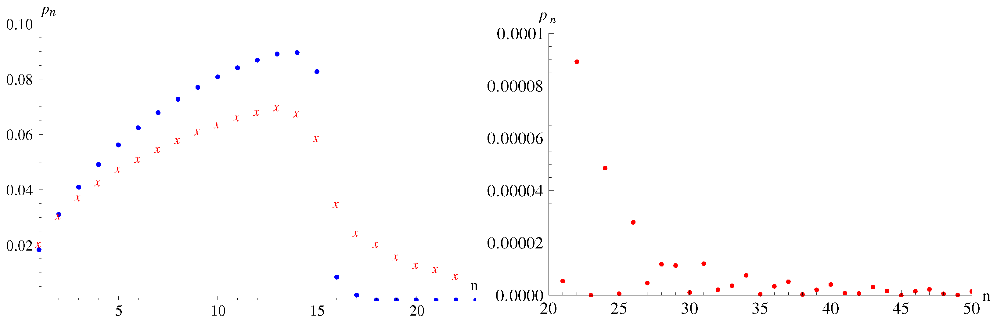
A comparison between the theoretical probabilities
and those obtained experimentally by Ichikawa et al. reveals significant discrepancies beyond the first two states (see
Figure 4). The experimental data from Ichikawa et al. [
27] show discrepancies with the spatial distribution of quantum gravitational states predicted theoretically. This conclusion is supported by further analysis using the Wigner function (see
Section 7).
7. Wigner Function for Quantum Gravitational States of
Ultracold Neutrons
In this section, we analyze the spatial distribution of quantum gravitational states of ultracold neutrons using the Wigner function [
28,
29], as performed by Ichikawa et al. [
27]. The Wigner function for the quantum gravitational states of ultracold neutrons in region III is defined by [
27]:
where
. The Wigner function
offers a quasi-probabilistic representation of quantum states, describing their coherence in both position and momentum space. The dependence on
arises from the geometrical scattering conditions and relates the vertical spatial distribution to the horizontal velocity component. By substituting
(see Equation (
6)) and
, where
is given by:
and using the expansion coefficients
and wave functions
, we rewrite the Wigner function in the following form:
where
is defined by Equation (
6), and the coefficients
and
are given by Equation (
21). The coefficients
, averaged over random phases
, are as follows:
where
,
,
, and
. The Wigner function given by Equation (
20) is plotted in
Figure 5.
After integrating the Wigner function (Equation (
20)) over velocities
using a Gaussian distribution, we obtain the following expression:
where
is the variance in the horizontal velocities of ultracold neutrons.The Gaussian approximation for the horizontal velocity distribution
reflects the experimental observations of ultracold neutron sources, where horizontal velocities exhibit a thermal spread. The contributions of the crossing terms
and
are negligible due to strong oscillations and the smallness of their amplitudes. Numerical simulations confirm that the oscillatory crossing terms average out over the integration range due to their high-frequency behavior. This ensures their contributions to
are negligible relative to the diagonal terms.
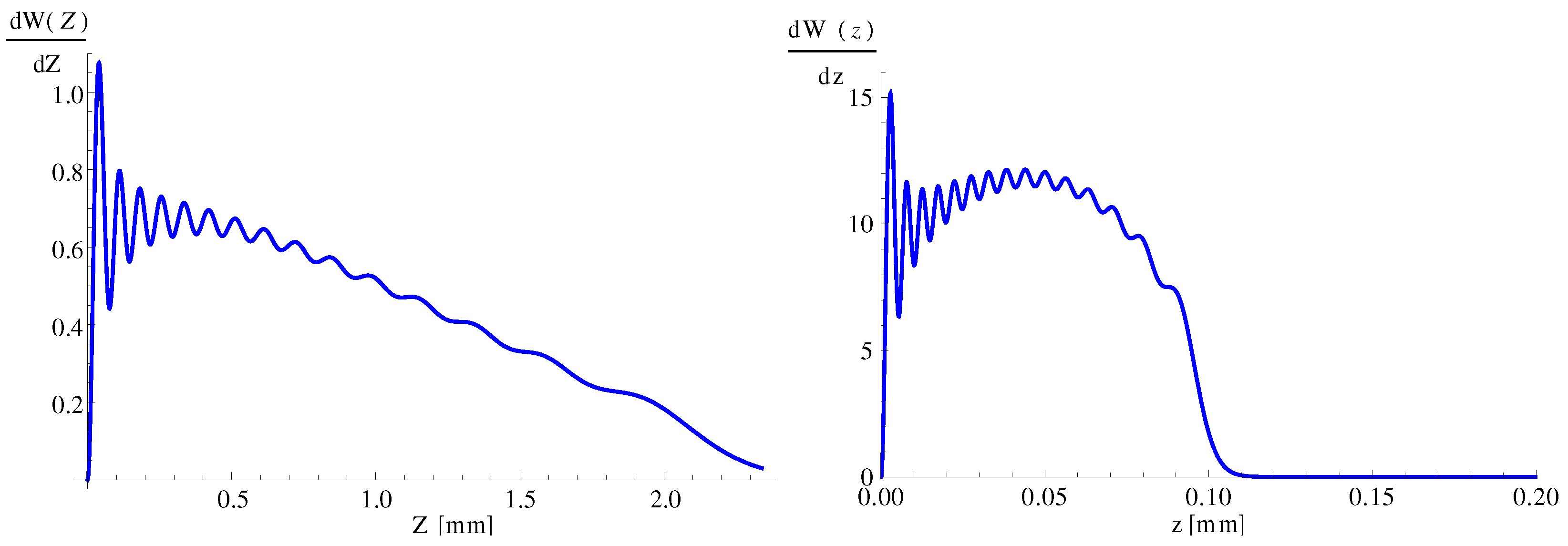
By replacing
and using Equation (
6), we obtain the spatial distribution of quantum gravitational states of ultracold neutrons in a pixelated detector in terms of the Wigner function
:
In
Figure 6 we plot the Wigner function
in the interval
.
8. Discussion
The results presented in this work highlight significant discrepancies between the theoretical predictions and experimental data on the spatial distribution of quantum gravitational states of ultracold neutrons obtained by Ichikawa et al. [
27]. While the theoretical framework accurately predicts the probabilities
and the corresponding wave functions in both regions II and III, the experimental data deviate substantially from these expectations, raising questions about their interpretation. We summarize the following key points and arguments:
Theoretical Consistency
The theoretical model relies on well-established quantum mechanical principles and boundary conditions for wave functions in confined regions. The wave functions and are derived rigorously using Airy functions, with roots calculated to a high precision. Furthermore, the completeness relation ensures that the total probability is conserved. This theoretical rigor results in spatial probability distributions that are self-consistent and numerically stable, particularly for the first 100 quantum gravitational states in region III.
Comparison with Experimental Data
The comparison between our theoretically derived probabilities and those reported by Ichikawa et al. reveals agreement only for the first two quantum gravitational states. Beyond these, the experimental probabilities deviate significantly, exhibiting trends that are neither consistent with quantum mechanical predictions nor indicative of random noise. These discrepancies suggest that the experimental data interpretation may not accurately capture the quantum behavior of ultracold neutrons.
Unexplained Oscillations in High States
The probabilities for higher quantum states () exhibit random oscillations, as predicted by our model, which are not observed in the experimental data by Ichikawa et al. These oscillations arise naturally from the orthogonality of wave functions and their overlap integrals, indicating a failure of the experimental setup to resolve or detect higher-order quantum gravitational states accurately.
Sensitivity to Initial Conditions
The wave functions in region II, , are highly sensitive to the precision of the roots . This sensitivity impacts the probabilities and their subsequent propagation into region III. Our analysis shows that minute deviations in these roots could lead to notable changes in the spatial distribution in region III. However, this effect does not account for the observed experimental discrepancies, which are far larger than what could be attributed to root precision.
Experimental Limitations and Systematic Errors
The experimental setup described by Ichikawa et al. might introduce systematic biases that are not adequately accounted for:
Beam Characteristics: The distribution of ultracold neutrons in the beam may not perfectly correspond to the assumed probability distribution , affecting the initial conditions in region II.
Detector Resolution: The pixelated detector used to project spatial distributions in region III may have insufficient resolution to accurately measure higher-order quantum states.
Uncontrolled Environmental Factors: Gravitational gradients, vibrations, or mirror imperfections in the experimental setup could distort the spatial distribution of ultracold neutrons.
Reevaluation of Experimental Assumptions
The interpretation of Ichikawa et al. implicitly assumes that the spatial distributions in region III directly reflect the mixed quantum state formed in region II. However, the complex dynamics at the boundary between regions II and III may introduce additional effects, such as decoherence or scattering, that are not accounted for in the experimental analysis. Such effects could explain the observed deviations from the theoretical predictions.
Wigner Function Analysis
As detailed in the previous section, the analysis of the Wigner function further supports the conclusion that the experimental data lack the expected quantum coherence. The Wigner function analysis reveals that the observed spatial distributions are inconsistent with the quantum mechanical predictions for mixed states of ultracold neutrons. This suggests that the experimental data may be dominated by classical or semiclassical effects, rather than pure quantum gravitational states.
In light of these arguments, it is evident that the experimental results reported by Ichikawa et al. do not align with the spatial distributions predicted by quantum mechanics for ultracold neutrons in gravitational fields. To resolve these discrepancies, further experimental investigations are required, with particular attention to the following:
Enhanced precision in beam preparation and state initialization in region II.
Improved resolution and calibration of the pixelated detector in region III.
A detailed study of environmental influences and systematic errors.
Additionally, theoretical models should be extended to include potential decoherence mechanisms and other perturbative effects that may arise at the interface between regions II and III. Such efforts would provide a more comprehensive understanding of the dynamics of ultracold neutrons in quantum gravitational states and bridge the gap between theory and experiment.
9. Conclusions
To construct a robust model for ultracold neutrons (UCNs) interacting with gravitational fields and cylindrical mirrors, it is essential to incorporate simplifying assumptions. A common assumption is that the UCN beam reaches a steady-state distribution. This simplifies the analysis by focusing on the time-independent behavior of the neutrons. Typically, the initial velocity distribution of UCNs follows a Maxwell–Boltzmann distribution at very low temperatures, as reported by [
27].
The interaction of neutrons with mirror surfaces involves complex phenomena such as absorption, reflection, and scattering. To simplify the model, we assume that the mirrors are ideal, perfectly reflective surfaces. This implies that neutrons undergo specular reflection, where the angle of incidence equals the angle of reflection, with no energy loss. This assumption is valid for mirrors that are smooth and highly reflective to UCNs, which is typically achieved by using specialized coatings designed for neutron reflectivity. By adopting this idealization, we avoid complications arising from microscopic surface properties or inelastic scattering processes, making the boundary conditions tractable mathematically.
We analyzed experimental data on the spatial distribution of quantum gravitational states of UCNs obtained by Ichikawa et al. [
27]. In their experimental setup, UCNs with a horizontal velocity
, following a Gaussian distribution with a mean velocity
and variance
, pass through three distinct regions:
A spatial region between two parallel mirrors (region II),
A spatial region above a mirror (region III),
A detection region, where UCNs are observed.
The cylindrical mirror projects UCNs from region III onto the detector.
Due to the small de Broglie wavelength of the neutrons,
, compared to both the distance between the two mirrors,
, and the radius of the cylindrical mirror,
, the scattering of UCNs by the cylindrical mirror can be treated classically. In this framework, the impact parameter
b of a neutron corresponds to its vertical coordinate
z. For analyzing the spatial distribution of UCNs on the detector, we project the impact parameter
b onto the detector variable
Z. For the experimental setup in [
27], UCNs are detected only within an interval
. The projection is defined such that UCNs with
are mapped to
.
To calculate the probability density distributions of quantum gravitational states of UCNs and the corresponding Wigner functions, we define the wave function of the mixed state in region II as a superposition of 15 quantum gravitational states. The expansion coefficients
(
) are determined by the
z-distribution of UCNs. The wave functions of these quantum gravitational states between the two mirrors have been previously computed in [
24].
When expanding the wave function of UCNs from region II into the quantum gravitational states in region III, we include up to 100 states, characterized by expansion coefficients (). This expansion satisfies the unitarity condition, , where averaging is performed over random phases of the coefficients in region II.
In
Figure 4, we show that the probabilities
for UCNs to occupy the
n-th quantum gravitational state differ significantly from those calculated by Ichikawa et al. [
27]. Specifically, the smooth dependence of
on
n for
, reported by Ichikawa et al., is inconsistent with our findings. The wave function of the mixed state is localized within
, leading to an irregular and oscillatory dependence of
on
n for
.
Our analysis also reveals that the calculated probability distributions (
Figure 5) and the Wigner function (
Figure 6) do not align with the experimental data from Ichikawa et al. [
27]. This discrepancy suggests that their data cannot be fully explained by the spatial distribution of quantum gravitational states of UCNs under our theoretical framework.
Author Contributions
D.A.: Conceptualization, Methodology, Data Curation, Formal analysis, Investigation, Writing—Original draft preparation. R.H.: Conceptualization, Formal analysis, Data Curation, Investigation, Methodology, Software, Validation, Writing—Original draft preparation. M.W.: Conceptualization, Formal analysis, Data Curation, Investigation, Methodology, Software, Validation, Writing—Original draft preparation. All authors contributed equally and agreed to the published version of the manuscript. The sole responsibility for the content of this publication lies with the authors.
Funding
The work of M. Wellenzohn was supported by MA 23 (p.n. 30-22).
Data Availability Statement
The data and illustrations presented in this study can be obtained directly from the equations. All data are available upon request from the corresponding author.
Acknowledgments
We want to acknowledge our dear colleague Andrey Nikolaevich Ivanov, who was the main investigator of this work until he sadly passed away on 18 December 2021. We see it as our professional and personal duty to honor his legacy by continuing to publish our collaborative work. Andrey was born on 3 June 1945 in what was then Leningrad. Since 1993 he was a university professor at the Faculty of Physics, named “Peter The Great St. Petersburg Polytechnic University” after Peter the Great. Since 1995 he has been a guest professor at the Institute for Nuclear Physics at the Vienna University of Technology for several years and has been closely associated with the institute ever since. This is also where we met Andrey and have been collaborating with him closely over more than 20 years, resulting in 40 scientific publications. We will miss Andrey as a personal friend for his immense wealth of ideas, scientific skills, and creativity. See also the official obituary for Andrey Nikolaevich Ivanov. The work of M. Wellenzohn was supported by MA 23 (p.n. 27-07 and p.n. 30-22). The sole responsibility for the content of this publication lies with the authors.
Conflicts of Interest
The authors declare no conflicts of interest.
References
- Gibbs, R.L. The quantum bouncer. Am. J. Phys. 1975, 43, 25. [Google Scholar] [CrossRef]
- Luschikov, V.I.; Frank, A.I. Quantum effects occurring when ultracold neutrons are stored on a plane. JETP Lett. 1978, 28, 559–561. [Google Scholar]
- Wallis, H.; Dalibard, J.; Cohen-Tannoudji, C. Trapping atoms in a gravitational cavity. Appl. Phys. B 1992, 54, 407. [Google Scholar] [CrossRef]
- Gea-Banacloche, J. A quantum bouncing ball. Am. J. Phys. 1999, 67, 776. [Google Scholar] [CrossRef]
- Abele, H. The neutron. Its properties and basic interactions. Prog. Part. Nucl. Phys. 2008, 60, 1–81. [Google Scholar] [CrossRef]
- Nesvizhevsky, V.V.; Börner, H.G.; Petukhov, A.K.; Abele, H.; Baeßler, S.; Rueß, F.J.; Stöferle, T.; Westphal, A.; Gagarski, A.M.; Petrov, G.A.; et al. Quantum states of neutrons in the Earth’s gravitational field. Nature 2002, 415, 297. [Google Scholar] [CrossRef] [PubMed]
- Nesvizhevsky, V.V.; Börner, H.G.; Petukhov, A.K.; Abele, H.; Baeßler, S.; Rueß, F.J.; Stöferle, T.; Westphal, A.; Strelkov, A.V.; Protasov, K.V.; et al. Measurement of quantum states of neutrons in the Earth’s gravitational field. Phys. Rev. D 2003, 67, 102002. [Google Scholar] [CrossRef]
- Nesvizhevsky, V.V.; Petoukhov, A.K.; Borner, H.G.; Protasov, K.V.; Voronin, A.Y.; Westphal, A.; Baessler, S.; Abele, H.; Gagarski, A.M. Reply to “Comment on ‘Measurement of quantum states of neutrons in the Earth’s gravitational field’”. Phys. Rev. D 2003, 68, 108702. [Google Scholar] [CrossRef]
- Abele, H.; Baessler, S.; Westphal, A. Quantum states of neutrons in the gravitational field and limits for non-Newtonian interaction in the range between 1 micron and 10 microns. Lect. Notes Phys. 2003, 631, 355. [Google Scholar]
- Nesvizhevsky, V.V.; Petukhov, A.K.; Börner, H.G.; Baranova, T.A.; Gagarski, A.M.; Petrov, G.A.; Protasov, K.V.; Voronin, A.Y.; Baeßler, S.; Abele, H.; et al. Study of the neutron quantum states in the gravity field. Eur. Phys. J. C 2005, 40, 479. [Google Scholar] [CrossRef]
- Voronin, A.Y.; Abele, H.; Baessler, S.; Nesvizhevsky, V.V.; Petukhov, A.K.; Protasov, K.V.; Westphal, A. Quantum motion of a neutron in a waveguide in the gravitational field. Phys. Rev. D 2006, 73, 044029. [Google Scholar] [CrossRef]
- Abele, H.; Baessler, S.; Borner, H.G.; Gagarsky, A.M.; Nesvizhevsky, V.V.; Petukhov, A.K.; Protasov, K.V.; Voronin, A.Y.; Westphal, A. Gravitationally bound quantum states of neutrons: Applications and perspectives. AIP Conf. Proc. 2006, 842, 793–795. [Google Scholar] [CrossRef]
- Westphal, A.; Abele, H.; Baessler, S.; Nesvizhevsky, V.V.; Petukhov, A.K.; Protasov, K.V.; Voronin, A.Y. A quantum mechanical description of the experiment on the observation of gravitationally bound states. Eur. Phys. J. C 2007, 51, 367–375. [Google Scholar] [CrossRef]
- Naganawa, N.; Ariga, T.; Awano, S.; Hino, M.; Hirota, K.; Kawahara, H.; Kitaguchi, M.; Mishima, K.; Shimizu, H.; Tada, S.; et al. Measurement of the W-boson mass in pp collisions at = 7 TeV with the ATLAS detector. Eur. Phys. J. C 2018, 78, 110. [Google Scholar]
- Muto, N.; Abele, H.; Ariga, T.; Bosina, J.; Hino, M.; Hirota, K.; Ichikawa, G.; Jenke, T.; Kawahara, H.; Kawasaki, S.; et al. A novel nuclear emulsion detector for measurement of quantum states of ultracold neutrons in the Earth’s gravitational field. J. Instrum. 2022, 17, P07014. [Google Scholar] [CrossRef]
- Nesvizhevsky, V.V.; Börner, H.; Gagarski, A.M.; Petrov, G.A.; Petukhov, A.K.; Abele, H.; Bäßler, S.; Stöferle, T.; Soloviev, S.M. Search for quantum states of the neutron in a gravitational field: Gravitational levels. Detect. Assoc. Equip. 2000, 827, 750. [Google Scholar] [CrossRef]
- Nesvizhevsky, V.V.; Protasov, K.; Moore, D.C. Trends in Quantum Gravity Research; Nova Science Publishers: New York, NY, USA, 2006; pp. 65–107. [Google Scholar]
- Abele, H.; Jenke, T.; Stadler, D.; Geltenbort, P. QuBounce: The dynamics of ultra-cold neutrons falling in the gravity potential of the Earth. Nucl. Phys. A 2009, 827, 593c. [Google Scholar] [CrossRef]
- Jenke, T.; Stadler, D.; Abele, H.; Geltenbort, P. Q-BOUNCE—Experiments with quantum bouncing ultracold neutrons. Nucl. Instr. Meth. Phys. Res. A 2009, 611, 318. [Google Scholar] [CrossRef]
- Baessler, S.; Gagarski, A.M.; Lychagin, E.V.; Mietke, A.; Muzychka, A.Y.; Nesvizhevsky, V.V.; Pignol, G.; Strelkov, A.V.; Toperverg, B.P.; Zhernenkov, K. New methodical developments for GRANIT. Comptes Rendus Phys. 2011, 12, 729. [Google Scholar] [CrossRef]
- Abele, H.; Leeb, H. Gravitation and quantum interference experiments with neutrons. New J. Phys. 2012, 14, 055010. [Google Scholar] [CrossRef]
- Jenke, T.; Geltenbort, P.; Lemmel, H.; Abele, H. Realization of a gravity-resonance-spectroscopy technique. Nat. Phys. 2011, 7, 468. [Google Scholar] [CrossRef]
- Jenke, T.; Cronenberg, G.; Burgdörfer, J.; Chizhova, L.A.; Geltenbort, P.; Ivanov, A.N.; Lauer, T.; Lins, T.; Rotter, S.; Saul, H.; et al. Gravity Resonance Spectroscopy Constrains Dark Energy and Dark Matter Scenarios. Phys. Rev. Lett. 2014, 112, 151105. [Google Scholar] [CrossRef]
- Ivanov, A.N.; Höllwieser, R.; Jenke, T.; Wellenzohn, M.; Abele, H. Influence of the chameleon field potential on transition frequencies of gravitationally bound quantum states of ultracold neutrons. Phys. Rev. D 2013, 87, 105013. [Google Scholar] [CrossRef]
- Mota, D.F.; Shaw, D.J. Strongly coupled chameleon fields: New horizons in scalar field theory. Phys. Rev. Lett. 2006, 97, 151102. [Google Scholar] [CrossRef] [PubMed]
- Brax, P.; Pignol, G. Strongly coupled chameleons and the neutronic quantum bouncer. Phys. Rev. Lett. 2011, 107, 111301. [Google Scholar] [CrossRef]
- Ichikawa, G.; Komamiya, S.; Kamiya, Y.; Minami, Y.; Tani, M.; Geltenbort, P.; Yamamura, K.; Nagano, M.; Sanuki, T.; Kawasaki, S.; et al. Observation of the Spatial Distribution of Gravitationally Bound Quantum States of Ultracold Neutrons and Its Derivation Using the Wigner Function. Phys. Rev. Lett. 2014, 112, 071101. [Google Scholar] [CrossRef] [PubMed]
- Wigner, E.P. On the Quantum Correction For Thermodynamic Equilibrium. Phys. Rev. 1932, 40, 749. [Google Scholar] [CrossRef]
- Hillery, M.; O’Connel, R.F.; Scully, M.O.; Wigner, E.P. Distribution functions in physics: Fundamentals. Phys. Rep. 1984, 106, 121. [Google Scholar] [CrossRef]
- Davydov, A.S. Quantum Mechanics; Pergamon Press: Oxford, UK, 1965. [Google Scholar]
- Landau, L.D.; Lifschitz, E.M. Lehrbuch der Theoretischen Physik; Akademie Verlag: Berlin, Germany, 1979. [Google Scholar]
- Ruess, F. Quantum States in the Gravitational Field. Diploma Thesis, Faculty of Physics and Astronomy, University of Heidelberg, Heidelberg, Germany, 2000. [Google Scholar]
| Disclaimer/Publisher’s Note: The statements, opinions and data contained in all publications are solely those of the individual author(s) and contributor(s) and not of MDPI and/or the editor(s). MDPI and/or the editor(s) disclaim responsibility for any injury to people or property resulting from any ideas, methods, instructions or products referred to in the content. |
© 2024 by the authors. Licensee MDPI, Basel, Switzerland. This article is an open access article distributed under the terms and conditions of the Creative Commons Attribution (CC BY) license (https://creativecommons.org/licenses/by/4.0/).


