1. Introduction
In quantum field theory regarding black hole (BH) spacetimes, particular relevance is given to the so-called ‘Unruh vacuum’ [
1]. This quantum state is defined using the maximal analytic extension of the BH spacetime by expanding the quantum field operators in ingoing modes that have a positive frequency with respect to asymptotic Minkowski time, whereas for the outgoing modes, emerging from the past horizon, these are chosen as a positive frequency with respect to Kruskal time. At late retarded time, this state is expected to describe the quantum state of a field in the spacetime of a collapsing body forming a BH.
Let us make an explicit example in the simple setting of a two-dimensional Schwarzschild spacetime, for which the metric reads
where
m is the BH mass and
are, respectively, the retarded and advanced Eddington–Finkelstein coordinates.
is the Regge–Wheeler ‘tortoise’ coordinate
Kruskal’s null co-ordinates are defined as [
2]
where
is the surface gravity of the BH horizon located at
.
The maximal analytic extension of the Schwarzschild metric is depicted in the Penrose diagram (see, for example, [
3]) in
Figure 1, describing an eternal Schwarzschild BH. In Equation (
5), the sign − holds in the asymptotically flat region
R and the white hole region
; the sign + is the BH region
and in
L. In (
6), the sign + refers to the
R and
regions, while it refers to − in
and
L. We shall limit our discussion to the physically interesting regions
R and
.
In this spacetime, we consider a massless scalar quantum field,
, minimally coupled to gravity, the field equation of which is
where
is the covariant D’Alembertian.
In order to obtain the Unruh vacuum, one expands the field as
The first term in Equation (
8) represents the ingoing part, while the second represents the outgoing version. Note that
U is locally inertial on
. The
’s are annihilation operators, and the Unruh vacuum
is defined as
for every
.
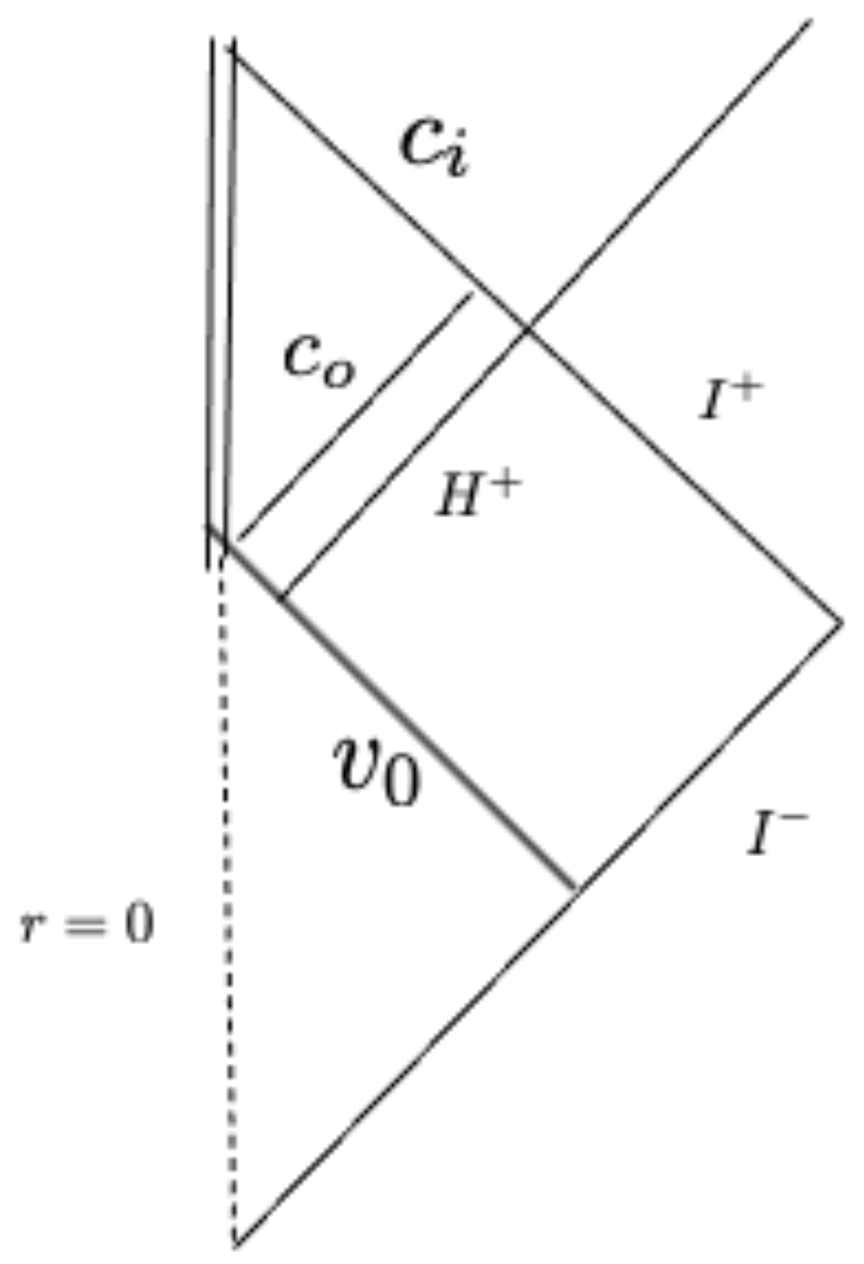
Now, consider a Schwarzschild BH formed by the collapse of a spherically symmetric star. The corresponding Penrose diagram is depicted in
Figure 2.
In this spacetime, we consider, as before, a quantum field , and we suppose the field is in a quantum state that corresponds to Minkowski vacuum on . We call this state ; in this state, there are no incoming particles (radiation) associated with .
Now,
in the spacetime of
Figure 1 approximates the behavior of
in the physical spacetime of
Figure 2 at late retarded time,
u. For a detailed discussion, see [
4]. In particular, when considering the energy momentum tensor operator
, in the Schwarzschild region, we have
As it is well known,
describes at
a thermal flux of radiation at the Hawking temperature
which is exactly what Hawking derived in 1974 [
5,
6] by computing the in-out Bogoliubov coefficients for the late time behavior of
. This is the reason for using the Unruh vacuum to describe Hawking’s BH radiation.
In this paper, we shall investigate the relation between the Unruh vacuum and the vacuum in the setting of a charged BH described by the Reissner-Nordström (RN) metric, both for non-extremal and extremal configurations.
2. Non-Extremal Reissner-Nordström Black Holes: The Unruh Vacuum
We focus our attention on an RN BH of mass
m and charge
Q. The BH is supposed to be non-extremal, i.e.,
. The metric describing it is
where, again,
but now
In this case, we have two horizons: an event horizon at
and an inner one at
where
and two corresponding surface gravities:
We have two possible ways to implement the construction of Kruskal coordinates, namely
which are regular on
but not on
where they diverge, or [
7]
where they are regular on
but singular on
where they diverge.The Penrose diagram of the maximally extended RN solution is given in
Figure 3.
In the regions of our interest, we have indicated as the future event horizon () and as the past one (). The Cauchy horizon, , is located at : is the outgoing sheet () while is the ingoing version ().
The Unruh vacuum is usually constructed out of
, namely expanding the field as
and the Unruh vacuum
is defined by
for every
.
We shall focus on the renormalized expectation values of
[
8,
9,
10] in this state, which read [
11]
where
and a prime “
” indicates the derivative with respect to
r.
means Schwarzian derivative, and we obtain
This last term in Equation (
26) describes the Hawking radiation at
The other terms in Equations (
24)–(
26) represent the vacuum polarization contribution and correspond to the expectation values calculated in the so-called Boulware vacuum
[
12], obtained by expanding the field
in modes that are positive and negative infrequency with respect to
t, namely
. We can formally write Equations (
24)–(
26) as
where
with
The tensor
is conserved and describes radiation propagating along constant
u.
Mathematically, one can also define the Unruh vacuum associated with the Kruskal coordinate
of Equation (
20), i.e., expanding the field in outgoing modes of the form
. The resulting vacuum state, call it
, has the following expectation values of
where, as before,
but now
3. Non Extremal Reissner-Nordström Black Holes: The Vacuum
Let us now suppose that the RN BH is formed by the gravitational collapse of a charged body. We simplify the discussion by considering the collapse of a charged null shell. One can generalize this to an arbitrary body [
13].
The corresponding Penrose diagram is given in
Figure 4.
The spacetime metric of this model can be given as follows. The shell is located at
. For
, we have Minkowski spacetime:
where
are, respectively, the null outgoing and ingoing directions. From Equations (
38) and (
39), we have
For
, we have the RN metric
where
is given in Equation (
27) and
, and
in Equations (
13)–(
15). By matching the metric across
, we can relate the null outgoing coordinates
u and
[
14]:
We can extend the
co-ordinate in the RN region using the above relation. The event horizon
is located at
The inner horizon outgoing sheet
corresponds to
Note that this null surface, unlike the previous case of the maximal analytic extension of the RN spacetime (see
Figure 3), does not correspond to the outgoing sheet of the Cauchy horizon anymore (see
Figure 4). The latter is, indeed, shifted inside the BH and is located at (using the reflection condition at
, see Equation (
40))
Note that near
,
i.e.,
behaves as the Kruskal
of Equation (
18) up to a shift. When choosing, for example,
, they coincide. On the other side, near the outgoing sheet of the inner horizon (i.e., for
) we have
This means that
behaves like
(see Equation (
20)). So,
, unlike
, is a regular null outgoing coordinate both at
and at
). However, this coordinate is singular on the Cauchy horizon
, as can be seen from
where, from Equation (
42),
which vanishes like
for
. Note that
is nonvanishing neither on
nor on the outgoing sheet of
, making the
co-ordinates regular there, as stated before.
Note that past null infinity,
(see
Figure 4) is a Cauchy surface for our null field for the spacetime region within the Cauchy horizon
. The initial conditions on our field
on
determine its evolution in the above region. We choose the quantum state for our field to be a Minkowski vacuum on
. This is achieved by choosing the ingoing modes to be of the form
; the ougoing ones are simply the reflection through
(in the Minkowski part) of the incoming ones, namely of the form
, where the reflection condition sets
(see Equation (
40) at
). We call this quantum state
.
By using the standard formalism, we obtain
for
(i.e., in the Minkowski region), while for
, in the RN part, we obtain
where the last term in Equation (
53) is the Schwarzian derivative between
and
u to be calculated from Equation (
42)
where
. The following limiting behaviors are interesting. For
(i.e.,
), we have (see Equation (
46))
while for
(i.e.,
), see Equation (
47),
So, when comparing Equations (
51)–(
53) with the corresponding ones ((
24)–(
26) and (
34)), we can conclude that in the RN region,
and
So the Unruh vacuum
reproduces
at late (
) retarded time, while this does not happen at the inner horizon. There the
vacuum is well approximated by
.
4. Regularity
We shall consider a quantum state to be “regular” if the expectation values of in that given state are finite when expressed in a regular co-ordinate system. Support for this comes from the fact that the expectation values of in the semiclassical Einstein equations represent the source that drives the backreaction of the quantum fields in the spacetime metric.
Let us start with the Unruh vacuum
. The expectation values of
in this state are given by Equations (
24)–(
26), and one sees immediately that they diverge on the physical singularity located at
. However, the Eddington–Finkelstein co-ordinates,
, used in Equations (
24)–(
26) are singular on the horizons
. So, care must be taken when considering these regions.
We begin with
. A coordinate system regular there is the Kruskal one
of Equations (
18) and (
19). We require the finiteness of
as
when expressed in these Kruskal coordinates. This implies that on the event horizon
, we need the regularity of
(see [
15]) such that
Conditions
and
are easily satisfied using Equations (
25) and (
24), respectively. Concerning condition
, note that
So, according to Equation (
33), we see that
vanishes at
and also, as can be rapidly checked, its first derivative. This means that
vanishes as
for
, making condition
satisfied. So,
is regular on
. Regularity on
is given by conditions similar to Equations (
59)–(
61) but with
u and
v interchanged, namely
From Equations (
25) and (
26), we see that
and
are satisfied but not
. From Equation (
24), we see that
and, hence, condition
is not satisfied, as
. Hence,
is not regular on
.
We now come to the inner horizon, where for a regular coordinate system, this can be given by Kruskal’s
, as per Equations (
20) and (
21). The regularity conditions on the outgoing sheet of the Cauchy horizon
are given by the same requirements of Equations (
59)–(
61). One rapidly checks the fullfillement of Equations (
60) and (
61). Concerning (
59), we now have it that
implying that (see Equation (
33))
Because
, this is not vanishing, and condition (
59) is not fullfilled.
is not regular on
. The conditions for regularity on the ingoing sheet of the inner horizon
are given by Equations (
63)–(
65), and one checks that Equation (
63) is not satisfied for
since
is also singular on
[
16,
17] (see also [
18]).
A similar analysis can be performed on the state
(see Equations (
34)–(
36)), and we will see that
is not regular for the future horizon
, past horizon
, and also on the ingoing sheet of the inner horizon
, whereas it is regular on the outgoing sheet
.
We come now to the
state. In view of the previous discussion on the states
, and the relations of these with the
state found in
Section 3, we see the following behavior. On
, we see that
is regular since (see (
57))
and
is regular on
. On the inner horizon
, which is no longer the outgoing sheet of the Cauchy horizon, (see Equation (
58))
where we see that
, unlike
, is regular because
is. Furthermore, the nonregularity of
on the past horizon
and on the ingoing sheet of the inner horizon
is rapidly established since
and we have seen that
are not regular on these regions. As we have remarked when presenting the spacetime of the collapsing shell (see
Figure 4), the outgoing sheet of the Cauchy horizon is no longer located at
but is at
. In order to check regularity on this surface, we just need to examine the component of
in the Eddington–Finkelstein coordinates
since they are regular there. By examining Equations (
51)–(
53), we find that the Schwarzian derivative
entering in (
53) diverges as
, and all other terms in Equations (
51)–(
53) are finite (except at the singularity at
). We conclude that
is not regular on
.
5. Extremal Reissner-Nordström BHs
So far, we have considered non-extremal BHs, i.e., , but what happens if the BH is extremal?
Extremal BHs are very interesting objects; they also appear in supergravity theories [
19] and represent, in some sense, a stable ground state for these theories. For extremal BHs, the surface gravity vanishes (see Equation (
17) for
); therefore, they do not emit Hawking radiation. They can be considered the end state of the evaporation of a non-extremal BH when the
charge
Q is conserved during the process.
We shall now discuss how we can extend the results of our previous investigation to the extremal BH case. The extremal RN BH is characterized by the metric
where, as usual,
but now
Note the presence of the last term in (
76) compared to the non-extremal case. The Penrose diagram of the extremal RN BH is given in
Figure 5.
The inner and outer horizon now coincide at .
We start by considering the Unruh vacuum. If we simply look at the final expression for the expectation values of
in the state
(Equations (
24)–(
33)) and naively set
, hence
, we see that the Schwarzian derivative term (
28) vanishes, so the Unruh state coincides with the Boulware version, leading to
which only describes the vacuum polarization induced by the BH, and this seems consistent with the fact that extremal BHs do not give Hawking radiation.
It is easy to see that
is not regular on the horizon
[
20]. When we require regularity in the free-falling frame across the future horizon, we obtain conditions identical to Equations (
59)–(
61), and we see that (
59) is not satisfied since the denominator there now vanishes as
while the numerator is only
(see Equation (
79)). Similarly, one finds a singular behavior on the past horizon and on the Cauchy horizon. It is not yet clear if this singular behavior is an artifact of the two-dimensional theory [
21,
22].
Besides regularity issues, one can question if the limiting procedure we used to derive Equations (
77)–(
79), as the
limit of the non-extremal version (
24)–(
26) is correct. If we go back to the original definition of the Unruh state
, starting with the outgoing modes that are positive in frequency with respect to Kruskal
, we see that the Equation (
18) defining
in terms of Eddington–Finkelstein
u makes no sense if
. So, one may wonder if the stress tensor of Equations (
77)–(
79) really describes the behavior of an extremal RN BH at late retarded time after its formation, as, indeed, this happens for a non-extremal BH, as we saw in
Section 3. In order to answer this, one should investigate the formation of an extremal RN BH, then construct the corresponding
state, compute the expectation values of
in this state, and see if at late
u, they coincide with the predictions of Equations (
77)–(
79).
Therefore, consider the formation of an extremal RN BH, as we did before, via the collapse of a charged null shell. One could consider, instead, a generic collapse without changing our conclusions. The Penrose diagram is given in
Figure 6.
For
, we have Minkowski spacetime:
whereas for
, the extreme RN metric is given by Equation (
73). Matching across the shell located at
gives
The event horizon
is at
. The ingoing sheet of the Cauchy horizon
is at
, while the outgoing one
is at
. By using Equation (
83), one can calculate the Schwarzian derivative, and the complete stress tensor reads
When looking at the
component, we immediately see that it has an extra contribution with respect to the static vacuum polarization
of Equation (
79). This term represents the transient radiation created by the time-dependent collapse of the shell decaying at late retarded time
as
. However, near the horizon, we have
, so the two terms in Equation (
86) vanish with the same power law, and they are opposite in sign. This makes the crucial limit for the regularity condition on
, i.e., Equation (
59), satisfied [
23]:
So,
is regular on
. We conclude that
cannot represent the state of a quantum field emerging at late retarded time for a collapse forming an extremal RN BH.
Note that in order to obtain the nonvanishing term from the Schwarzian derivative, it is necessary to also keep the subleading logarithmic term in Equation (
83) in the limit
. The omission of it would result in a vanishing Schwarzian derivative, missing, therefore, the correct result.
1Finally, one can verify that is not regular on the ingoing sheet of the Cauchy horizon and on the outgoing version, , where the Schwarzian derivative diverges, like .
6. Conclusions
We have investigated two particularly interesting quantum states for a field that propagates in RN spacetime: the Unruh state
and the
state. They are defined in two different spacetime manifolds. The Unruh state
is defined on the maximal analytic extension of the RN metric (see
Figure 3). It is a mathematical manifold. The
state is defined on the manifold associated with the formation of an RN BH (see
Figure 4). This is the physical manifold. We have seen if and when the Unruh state
can mimic the behavior of the physical state
.
These two states differ according to the choice of outgoing modes in the expansion of the field operator, while the ingoing ones are identical. For the Unruh vacuum, for a non-extremal BH, the outgoing modes have a positive frequency with respect to Kruskal’s null retarded co-ordinate
(see Equation (
18)). This co-ordinate is locally inertial on the past horizon
. On the other hand, for the
vacuum, the outgoing modes are simply the reflection of the ingoing ones at the center of the collapsing body. The incoming modes, in this case, are chosen in a way that the corresponding vacuum
coincides past null infinity
(which is a Cauchy surface), with a Minkowski vacuum. One can see that the definition of the
vacuum has a very solid physical motivation; it is not just a mathematical construction.
We have seen that for a non-extremal BH,
approximates very well
at late retarded time (
): this means near the horizon,
, and asymptotically at late-time. This motivates the use of the Unruh vacuum to discuss BH evaporation. However, although it is certainly true that the agreement between the two states is quite good near the horizon
, this is no longer true as soon as one moves inside the BH. While both states are regular on the event horizon
, the Unruh vacuum is singular on the outgoing sheet of the inner horizon at
for the maximal analytic extension of the RN metric. The state
, on the other hand, is perfectly regular on this outgoing null surface, which is no longer a Cauchy horizon for the collapse spacetime manifold of
Figure 4. For this physical spacetime, the outgoing sheet of the Cauchy horizon is shifted inside the inner horizon
at
, where
is singular. Note that in the maximal analytic extension, this surface is completely regular and has no particular physical significance. From Equation (
53), we see that it is the Schwarzian derivative term that diverges as
for the state
. This term represents the radiation emitted by the shell during its collapse. We see that this flux diverges as the shell radius goes to zero, meaning we have a thunderbolt null singularity [
26,
27].
Concerning the inner sheet of the Cauchy horizon, located for both spacetimes at
, we see that
and
are both irregular, making the full Cauchy horizon singular. One expects large backreaction effects (through the semiclassical Einstein equations) to occur there, leading to the formation of a spacetime singularity, as predicted by the mass inflation mechanism [
28,
29].
We finally analyzed the case of an extreme BH. It is often said that the Unruh vacuum (and also the Hartle–Hawking–Israel version [
30,
31]) coincides with the Boulware version since the surface gravity of these BHs horizons is vanishing. One may further support this idea by remarking on the fact that the Unruh vacuum is constructed by outgoing modes that are positive in frequency with respect to a null co-ordinate (
for a non-extremal BH), which is locally inertial on the past horizon. For an extremal RN BH, the Eddington–Finkelstein
u is locally inertial on the past horizon, and the outgoing modes of the Boulware vacuum are, indeed, positive in frequency with respect to
u. However, we have clearly shown that this Boulware vacuum for an extremal BH does not correctly describe (at a large
u) the physical state of a quantum field if the extreme RN BH is formed by the collapse of a star. So, its physical significance is quite unclear, and the results for extremal BHs obtained by simply taking the
limit of the expressions calculated for the Unruh or Hartle–Hawking–Israel states in non-extremal BHs should be regarded with suspicion.


