Investigating Fully Strange Tetraquark System with Positive Parity in a Chiral Quark Model

Abstract

Motivated by the intriguing discovery of $X\left(6900\right)$ by the LHCb collaboration, we undertake a comprehensive study of the $s\overline{s}s\overline{s}$ tetraquark system with positive parity, employing the Gaussian expansion within the chiral quark model method. We consider two structures, the diquark–antidiquark ($ss$-$\overline{s}\overline{s}$) structure and meson–meson ($s\overline{s}$-$s\overline{s}$) structure, covering all conceivable color and spin configurations. Despite the absence of bound states in our calculations, we have identified potential resonant states with $J^P=0^{+}$, namely, $R(0,2150)$ and $R(0,2915)$, as well as a resonant state with $J^P=1^{+}$, denoted as $R(1,2950)$, and a resonant state with $J^P=2^{+}$, denoted as $R(2,2850)$, utilizing the real-scaling method. By comparing their energies and widths, we suggest that $R(0,2915)$ and $R(1,2950)$ may share characteristics with $X\left(6900\right)$, while $R(0,2150)$ could be a promising candidate for the experimental state $f_0\left(2100\right)$. We strongly advocate for experimental investigations to shed light on the existence and properties of these resonant states.

1. Introduction

Since its initial discovery by the Belle Collaboration in 2003 [1], the $X\left(3872\right)$ state has garnered significant attention on the $c\overline{q}q\overline{c}$ structure. There is a lot of work on the $c\overline{q}q\overline{c}$ structure, such as $Y\left(4260\right)$ [2], $Z_c\left(3900\right)$ [3], $Y\left(4660\right)$ [4], and so on. Now, researchers have extensively investigated various structures involving heavy quarks and antiquarks, denoted by $Q\overline{q}q\overline{Q}$, within exotic tetraquark states. Examples include the possibility of $Y\left(4274\right)$ as a $c\overline{s}s\overline{c}$ structure, $D_{s0}^{\ast }\left(2317\right)$ as a $c\overline{q}q\overline{s}$ configuration, and $\mathsf{{\rm Y}}\left(10753\right)$ as a $b\overline{q}q\overline{b}$ state, as can be found in Refs. [5,6,7]. These studies have significantly contributed to a deeper understanding of QCD. Recently, the LHCb collaboration [8] reported $X\left(6900\right)$, sparking renewed interest in the $c\overline{c}c\overline{c}$ system. Subsequent reports have unveiled additional resonant states in the $c\overline{c}c\overline{c}$ spectrum, including $X\left(6600\right)$, $X\left(7200\right)$, and so on [9,10]. However, it is noteworthy that while $c\overline{c}c\overline{c}$ states with positive parity have been extensively explored in the literature, there has been comparatively less attention on $s\overline{s}s\overline{s}$ states with positive parity.

Studies of the $s\overline{s}s\overline{s}$ configuration may be traced back to the discovery of $Y\left(2175\right)$ in 2006 [11], which is now known as $\varphi \left(2170\right)$, in the initial state radiation (ISR) process of $e^{+}{e}^{-}\to {\gamma }_{ISR}\varphi {\pi }^{+}{\pi }^{-}$. The mass of this state is measured to be $2163\pm 7$ MeV/$c^2$, with a width of ${103}_{-21}^{+28}$ MeV/$c^2$. The BESIII collaboration [12] recently reported the discovery of a novel resonance, named $X\left(2100\right)$, in the $\varphi {\eta }^{\prime }$ invariant mass distribution. The resonance’s quantum numbers remain under scrutiny. Assuming $J^P=1^{+}$, the measured mass is $2062.8\pm 13.1\left(\mathrm{stat}\right)\pm 4.2\left(\mathrm{syst}\right)$ MeV/$c^2$ and the decay width is $177\pm 36\left(\mathrm{stat}\right)\pm 20\left(\mathrm{syst}\right)$ MeV/$c^2$. Conversely, for $J^P=1^{-}$, the mass is determined to be $2002.1\pm 27.5\left(\mathrm{stat}\right)\pm 15.0\left(\mathrm{syst}\right)$ MeV/$c^2$, with a corresponding width of ${103}_{-21}^{+28}\left(\mathrm{stat}\right)$ MeV/$c^2$. The quoted uncertainties are statistical and systematic, respectively. Furthermore, recent reports from the BESIII collaboration have shed light on two distinct resonances: $X\left(2500\right)$, observed in the context of $J/\psi \to \gamma \varphi \varphi$ [13], and the recently discovered $X\left(2239\right)$ resonance within the $e^{+}{e}^{-}\to K^{+}{K}^{-}$ process [14]. These discoveries have significantly expanded the $s\overline{s}s\overline{s}$ family. However, as of yet, the existence of clear positive parity $s\overline{s}s\overline{s}$ states remains elusive.

Current theoretical research is prominently focused on the $s\overline{s}s\overline{s}$ tetraquark state, particularly exploring its negative parity aspects. In Ref. [15], the author presented standard criteria within the QCD sum rules approach and conducted a comprehensive phenomenological analysis. The author suggests that $Y\left(2175\right)$ potentially may consist of color octet constituents rather than diquark pairs. Similarly, in Ref. [16], Chen et al. employed the QCD sum rule framework, constructing both diquark–antidiquark currents $\left(ss\right)\left(\overline{s}\overline{s}\right)$ and meson–meson currents $\left(s\overline{s}\right)\left(s\overline{s}\right)$. They extensively studied the decay properties of $Y\left(2175\right)$. Based on this work, Chen et al. recently utilized two independent $ss\overline{s}\overline{s}$ interpolating currents with $J^{PC}=1^{--}$, calculating both their diagonal and off-diagonal correlation functions. This calculation yielded two distinct physical states, one being $Y\left(2175\right)$ and the other at an energy level near 2.41 GeV/$c^2$, consistent with recent experimental observations [17]. Additionally, researchers investigated the mass spectrum of the $ss\overline{s}\overline{s}$ tetraquark states within the relativized quark model, incorporating screening effects. Notably, the observed resonance at 2239 MeV/$c^2$ could potentially correspond to a wave $1^{--}$$ss\overline{s}\overline{s}$ tetraquark state [18]. On the other hand, studies pertaining to the $ss\overline{s}\overline{s}$ tetraquark state with positive parity have also made significant progress. Deng et al. [19] utilized a chiral quark model to calculate the properties of the efficient $ss\overline{s}\overline{s}$ tetraquark state. Their results indicated that the $0^{+}$ state had an energy of approximately 1925 MeV/$c^2$, suggesting a candidate for $f_0\left(2020\right)$. In the QCD sum rule framework (Chen et al., Refs. [20,21]), calculations for quantum numbers $0^{++}$, $1^{+-}$, $2^{++}$ of the $ss\overline{s}\overline{s}$ four-quark state were conducted, yielding energies around 2.0 GeV/$c^2$. Additionally, quantum numbers $0^{-+}$ and $2^{-+}$ were associated with energies of approximately $2.{45}_{-0.24}^{+0.20}$ GeV/$c^2$ and $3.{07}_{-0.33}^{+0.25}$ GeV/$c^2$, respectively. The energy of the $1^{+-}$ tetraquark state aligned with results available in the literature [22,23].

In this investigation, the Gaussian expansion method (GEM) is applied to calculate the $s\overline{s}s\overline{s}$ tetraquark system with $J^P=0^{+},1^{+},2^{+}$. Two configurations are explored: a molecular $s\overline{s}$-$s\overline{s}$ and a diquark $ss$-$\overline{s}\overline{s}$ structure. Within the quark model framework, each energy eigenvalue in the diquark and color octet configurations corresponds to a stable bound state. However, the Gaussian expansion method used in our work yields a larger number of energy eigenvalues than those observed in experiments. To address this, the real-scaling (stabilization) method is implemented to identify genuine stable eigenvalues. Considering both experimental and theoretical evidence that the energies of discovered resonant states with the $s\overline{s}s\overline{s}$ configuration are below 3 GeV/$c^2$, our focus is specifically on $s\overline{s}s\overline{s}$ configurations with energies below 3 GeV/$c^2$.

The structure of this paper is organized as follows: In Section 1, we provide an introduction to the study. In Section 2, we elaborate on the details of the chiral quark model (ChQM) and GEM employed in our investigation. Subsequently, in Section 3, we describe a method for identifying and calculating the decay width of the genuine resonance state. In Section 4, we present the numerical results. Finally, in Section 5, we summarize our findings and conclude this work.

2. Chiral Quark Model, Wave Function of $\mathbf{s}\overline{\mathbf{s}}\mathbf{s}\overline{\mathbf{s}}$ System

2.1. Chiral Quark Model

The chiral quark model, a well-established theoretical framework renowned for its success in describing hadron spectra and hadron–hadron interactions, has been instrumental in shaping our approach in this study. Interested readers are encouraged to refer to the comprehensive details of the model available in Refs. [24,25,26]. In the exploration of the low-lying S-wave positive-parity $s\overline{s}s\overline{s}$ tetraquark system presented herein, only the central and spin–spin terms of the potential are taken into consideration. The Hamiltonian of the chiral quark model can be written as

$$\begin{array}{ccc}\hfill H& =& \sum _{i=1}^n(m_i+\frac{{\overrightarrow{p}}_i^2}{2m_i}-T_{CM})+\sum _{i<j=1}^n[V_{con}\left(r_{ij}\right)\hfill \\ & +& V_{oge}\left(r_{ij}\right)+\sum _{\chi =\pi ,\eta ,K}{V}_{\chi }\left(r_{ij}\right)],\hfill \end{array}$$

(1)

where $m_i$ is the constituent mass the of i-th quark (antiquark), $\frac{{\overrightarrow{p}}_i^2}{2m_i}$ is the kinetic energy of the i-th quark (antiquark), and $T_{CM}$ is the centroid kinetic energy. $r_{ij}$ refers to the relative coordinates between the i-th and j-th quark (antiquark). The energy of the whole system needs to be subtracted from the kinetic energy of the center of mass, so it is necessary to reduce the term ${\sum }_{i=1}^n(\frac{{\overrightarrow{p}}_i^2}{2m_i}-T_{CM})$ to three kinetic energy forms of relative motion, $\frac{{\overrightarrow{p}}_{12}^2}{2{\mu }_{12}}$, $\frac{{\overrightarrow{p}}_{34}^2}{2{\mu }_{34}}$, and $\frac{{\overrightarrow{p}}_{1234}^2}{2{\mu }_{1234}}$. And ${\mu }_{ij}$ is the reduced mass of two interacting quarks or quark clusters.

$$\begin{array}{ccc}\hfill {\mu }_{12}& =& \frac{m_1{m}_2}{m_1+m_2},{\mu }_{34}=\frac{m_3{m}_4}{m_3+m_4},\hfill \\ \hfill {\mu }_{1234}& =& \frac{(m_1+m_2)(m_3+m_4)}{m_1+m_2+m_3+m_4},\hfill \\ \hfill {\overrightarrow{p}}_{12}& =& \frac{m_2{\overrightarrow{p}}_1-m_1{\overrightarrow{p}}_2}{m_1+m_2},{\overrightarrow{p}}_{34}=\frac{m_4{\overrightarrow{p}}_3-m_3{\overrightarrow{p}}_4}{m_3+m_4},\hfill \\ \hfill {\overrightarrow{p}}_{1234}& =& \frac{(m_3+m_4){\overrightarrow{p}}_{12}-(m_1+m_2){\overrightarrow{p}}_{34}}{m_1+m_2+m_3+m_4},\hfill \\ \hfill T_{CM}& =& \frac{{({\overrightarrow{p}}_1+{\overrightarrow{p}}_2+{\overrightarrow{p}}_3+{\overrightarrow{p}}_4)}^2}{2(m_1+m_2+m_3+m_4)}.\hfill \end{array}$$

(2)

$V_{con}\left(r_{ij}\right)$ is the confining potential, which mimics the “confinement” property of QCD. Lattice-regularized QCD [27] has shown that multi-gluon exchanges result in an attractive linearly rising potential, proportional to the distance between infinitely heavy quarks. So we can phenomenologically describe the property by

$$V_{con}\left(r_{ij}\right)=(-a_c{r}_{ij}^2-\mathsf{\Delta }){\mathit{\lambda }}_i^c·{\mathit{\lambda }}_j^c$$

(3)

where ${\mathit{\lambda }}^c$ are $SU\left(3\right)$ color Gell–Mann matrices, and $a_c$ and ${\mu }_c$ are model parameters. The second potential $V_{oge}\left(r_{ij}\right)$ a one-gluon exchange interaction, reflecting the “asymptotic freedom” property of QCD, which includes the so-called Coulomb and color-magnetic interactions, is the leading-order contribution:

$$\begin{array}{ccc}\hfill V_{oge}\left(r_{ij}\right)& =& \frac{{\alpha }_s}{4}{\mathit{\lambda }}_i^c·{\mathit{\lambda }}_j^c\left[\frac{1}{r_{ij}}-\frac{2\pi }{3m_i{m}_j}{\mathit{\sigma }}_i·{\mathit{\sigma }}_j\delta \left({\mathbf{r}}_{ij}\right)\right],\hfill \end{array}$$

(4)

where $\mathit{\sigma }$ represents the $SU\left(2\right)$ Pauli matrices. And $r_0\left({\mu }_{ij}\right)=\frac{r_0}{{\mu }_{ij}}$, where $r_0\left({\mu }_{ij}\right)$ is upon the reduced mass of a quark–antiquark pair, ${\mu }_{ij}$. Additionally, the regularized contact term is expressed as

$$\begin{array}{c}\hfill \delta \left({\mathit{r}}_{ij}\right)=\frac{e^{-r_{ij}/r_0\left({\mu }_{ij}\right)}}{4\pi r_{ij}{r}_0^2\left({\mu }_{ij}\right)}.\end{array}$$

A scale-dependent strong coupling constant ${\alpha }_s$ that is effective over the light to heavy quark sector range provides a consistent description of mesons and baryons.

$${\alpha }_s\left({\mu }_{ij}\right)=\frac{{\alpha }_0}{ln\left[({\mu }_{ij}^2+{\mu }_0^2)/{\mathrm{\Lambda }}_0^2\right]}.$$

(5)

The third potential $V_{\chi }\left(r_{ij}\right)$ is the Goldstone boson exchange, coming from “chiral symmetry spontaneous breaking” of QCD in the low-energy region,

$$\begin{array}{ccc}\hfill V_{\pi }\left(r_{ij}\right)& =& \frac{g_{ch}^2}{4\pi }\frac{m_{\pi }^2}{12m_i{m}_j}\frac{{\mathrm{\Lambda }}_{\pi }^2}{{\mathrm{\Lambda }}_{\pi }^2-m_{\pi }^2}{m}_{\pi }[Y\left(m_{\pi }{r}_{ij}\right)-\hfill \\ & & \frac{{\mathrm{\Lambda }}_{\pi }^3}{m_{\pi }^3}Y\left({\mathrm{\Lambda }}_{\pi }{r}_{ij}\right)]{\mathit{\sigma }}_i·{\mathit{\sigma }}_j\sum _{a=1}^3{\lambda }_i^a{\lambda }_j^a,\hfill \\ \hfill V_K\left(r_{ij}\right)& =& \frac{g_{ch}^2}{4\pi }\frac{m_K^2}{12m_i{m}_j}\frac{{\mathrm{\Lambda }}_K^2}{{\mathrm{\Lambda }}_K^2-m_K^2}{m}_K[Y\left(m_K{r}_{ij}\right)-\hfill \\ & & \frac{{\mathrm{\Lambda }}_K^3}{m_K^3}Y\left({\mathrm{\Lambda }}_K{r}_{ij}\right)]{\mathit{\sigma }}_i·{\mathit{\sigma }}_j\sum _{a=1}^3{\lambda }_i^a{\lambda }_j^a,\hfill \\ \hfill V_{\eta }\left(r_{ij}\right)& =& \frac{g_{ch}^2}{4\pi }\frac{m_{\eta }^2}{12m_i{m}_j}\frac{{\mathrm{\Lambda }}_{\eta }^2}{{\mathrm{\Lambda }}_{\eta }^2-m_{\eta }^2}{m}_{\eta }[Y\left(m_{\eta }{r}_{ij}\right)-\hfill \\ & & \frac{{\mathrm{\Lambda }}_{\eta }^3}{m_{\eta }^3}Y\left({\mathrm{\Lambda }}_{\eta }{r}_{ij}\right)]{\mathit{\sigma }}_i·{\mathit{\sigma }}_j[{\lambda }_i^8{\lambda }_j^{8}cos{\theta }_P-{\lambda }_i^0{\lambda }_j^{0}sin{\theta }_P],\hfill \\ \hfill V_{\sigma }\left(r_{ij}\right)& =& -\frac{g_{ch}^2}{4\pi }\frac{{\mathrm{\Lambda }}_{\sigma }^2}{{\mathrm{\Lambda }}_{\sigma }^2-m_{\sigma }^2}{m}_{\sigma }[Y\left(m_{\sigma }{r}_{ij}\right)-\frac{{\mathrm{\Lambda }}_{\sigma }}{m_{\sigma }}Y\left({\mathrm{\Lambda }}_{\sigma }{r}_{ij}\right)],\hfill \end{array}$$

(6)

where $Y\left(x\right)=\frac{e^{-x}}{x}$ represents the Yukawa function and ${\lambda }^a$ denotes the $SU\left(3\right)$ flavor Gell–Mann matrices. The masses of Goldstone bosons are denoted by $m_{\pi }$, $m_{\eta }$, and $m_K$, while $m_{\sigma }$ is determined by the relation $m_{\sigma }^2\approx m_{\pi }^2+4m_{u,d}^2$. ${\mathrm{\Lambda }}_{\chi }$ serves as the cut-off, and $g_{ch}^2/4\pi$ stands for the Goldstone–quark coupling constant. This constant is determined from the $\pi NN$ coupling constant [28] via $\frac{g_{ch}^2}{4\pi }=\frac{9}{25}\frac{g_{\pi NN}^2}{4\pi }\frac{m_{u,d}^2}{m_N^2}$.

All the parameters are determined by fitting the meson spectrum, from light to heavy, taking into account only a quark=-antiquark component. They are shown in

Table 1. Quark model parameters ($m_{\pi }=0.7$ $f{m}^{-1}$, $m_{\sigma }=3.42$ $f{m}^{-1}$, $m_{\eta }=2.77$ $f{m}^{-1}$, $m_K=2.51$ $f{m}^{-1}$).

Quark masses	$m_u=m_d$(MeV/$c^2$)	313
	$m_s$(MeV/$c^2$)	536
	$m_c$(MeV/$c^2$)	1728
	$m_b$(MeV/$c^2$)	5112
Goldstone bosons	${\mathrm{\Lambda }}_{\pi }={\mathrm{\Lambda }}_{\sigma }\left(f{m}^{-1}\right)$	4.2
	${\mathrm{\Lambda }}_{\eta }={\mathrm{\Lambda }}_K\left(f{m}^{-1}\right)$	5.2
	$g_{ch}^2/\left(4\pi \right)$	0.54
	${\theta }_p{(}^{\circ })$	−15
Confinement	$a_c$($f{m}^{-2}·$ MeV/$c^2$)	101
	$\mathsf{\Delta }$(MeV/$c^2$)	−78.3
OGE	${\alpha }_0$	3.67
	${\mathrm{\Lambda }}_0\left(f{m}^{-1}\right)$	0.033
	${\mu }_0$(MeV/$c^2$)	36.976
	${\widehat{r}}_0$(MeV/$c^2$)	28.17

.

2.2. The Wave Function of $s\overline{s}s\overline{s}$ System

There are two physically important structures, meson–meson and diquark–antidiquark, considered in the present calculation. The wave functions of every structure consist of four parts: orbital, spin, flavor, and color. The wave function of each part is constructed in two steps, first write down the two-body wave functions, then coupling two subclusters’ wave functions to form the four-body one. Because there are two identical quark pairs in the system, the total wave function for the $s\overline{s}s\overline{s}$ system will be the tensor product of the orbital ($|R_i\rangle$), spin ($|S_j\rangle$), color ($|C_k\rangle$), and flavor ($|F_n\rangle$) components with necessary coupling,

$$|ijkn\rangle =\mathcal{A}\left[\right|R_i\rangle \otimes |S_j\rangle ]\otimes |C_k\rangle \otimes |F_n\rangle .$$

(7)

where $\mathcal{A}$ is the antisymmetrization operator. For the $s\overline{s}s\overline{s}$ system, $\mathcal{A}=1-P_{13}-P_{24}+P_{13}{P}_{24}$, where $P_{ij}$ refers to the antisymmetric operator.

2.2.1. Orbital Wave Function

The orbital wave function of the four-quark system consists of two subcluster orbital wave functions and the relative motion wave function between two subclusters (1, 3 denote quarks and 2, 4 denote antiquarks),

$$\begin{array}{ccc}\hfill |R_1\rangle & =& {\left[{\left[{\mathrm{\Psi }}_{l_1=0}\left({\mathbf{r}}_{12}\right){\mathrm{\Psi }}_{l_2=0}\left({\mathbf{r}}_{34}\right)\right]}_{l_{12=0}}{\mathrm{\Psi }}_{L_r}\left({\mathbf{r}}_{1234}\right)\right]}_{L=0},\hfill \\ \hfill |R_2\rangle & =& {\left[{\left[{\mathrm{\Psi }}_{l_1=0}\left({\mathbf{r}}_{13}\right){\mathrm{\Psi }}_{l_2=0}\left({\mathbf{r}}_{24}\right)\right]}_{l_{12=0}}{\mathrm{\Psi }}_{L_r}\left({\mathbf{r}}_{1324}\right)\right]}_{L=0},\hfill \end{array}$$

(8)

where the bracket “[ ]” indicates orbital angular momentum coupling, and L is the total orbital angular momentum which comes from the coupling of $L_r$, the orbital angular momentum of relative motion, and $l_{12}$, which is the from the coupling of $l_1$ and $l_2$, the subcluster orbital angular momenta. Given our focus on investigating the tetraquark state of $s\overline{s}s\overline{s}$ with positive parity, we set all of the orbital angular momenta to zero. $|R_1\rangle$ donates the orbital wave functions of the meson–meson structure, and $|R_2\rangle$ donates the wave functions of the diquark–antidiquark structure.

In order to describe the orbital wave function of the tetraquark system well, the GEM [29] is adopted. This method was initially proposed by Kamimura [30] and has been successfully applied in few-body calculations. It accurately describes short-range correlations, long-range asymmetric behavior, and the high oscillator character of wave functions in both bound and scattering states of the systems. In GEM, the radial part of the orbital wave function is expanded by a set of Gaussians:

$$\begin{array}{cc}\hfill \mathrm{\Psi }\left(\mathbf{r}\right)& =\sum _{n=1}^{n_{\max }}{c}_n{\psi }_{nlm}^G\left(\mathbf{r}\right),\hfill \end{array}$$

(9a)

$$\begin{array}{cc}\hfill {\psi }_{nlm}^G\left(\mathbf{r}\right)& =N_{nl}{r}^l{e}^{-{\nu }_n{r}^2}{Y}_{lm}\left(\widehat{\mathbf{r}}\right),\hfill \end{array}$$

(9b)

where $N_{nl}$ are normalization constants,

$$\begin{array}{c}\hfill N_{nl}={\left[\frac{2^{l+2}{\left(2{\nu }_n\right)}^{l+\frac{3}{2}}}{\sqrt{\pi }(2l+1)}\right]}^{\frac{1}{2}}.\end{array}$$

(10)

$c_n$ are the variational parameters, which are determined dynamically. The Gaussian size parameters are chosen according to the following geometric progression:

$${\nu }_n=\frac{1}{r_n^2},r_n=r_1{a}^{n-1},a={\left(\frac{r_{n_{\max }}}{r_1}\right)}^{\frac{1}{n_{\max }-1}}.$$

(11)

This procedure enables optimization of the use of Gaussians; as small as possible Gaussians are used. Since all of the orbital angular momenta in a tetraquark system are equal to 0, our Gaussians’ wave functions here can be simplified to

$${\psi }_{nlm}^G\left(\mathbf{r}\right)={\left[\frac{4{\left(2{\nu }_n\right)}^{\frac{3}{2}}}{\sqrt{\pi }}\right]}^{\frac{1}{2}}{e}^{-{\nu }_n{r}^2}\frac{1}{\sqrt{4\pi }}.$$

(12)

2.2.2. Spin Wave Function

Because there is no difference between the spin of a quark and antiquark, the meson–meson structure has the same spin wave function as the diquark–antidiquark structure. The spin wave functions of the subcluster are shown below.

$$\begin{array}{cc}\hfill & {\chi }_{11}^{\sigma }=\alpha \alpha ,{\chi }_{10}^{\sigma }=\frac{1}{\sqrt{2}}(\alpha \beta +\beta \alpha ),{\chi }_{1-1}^{\sigma }=\beta \beta ,\hfill \\ \hfill & {\chi }_{00}^{\sigma }=\frac{1}{\sqrt{2}}(\alpha \beta -\beta \alpha ).\hfill \end{array}$$

In the context of quark spin, $\alpha$ and $\beta$ represent the third component of quark spin, taking values of $\frac{1}{2}$ and $-\frac{1}{2}$, respectively, in the two distinct cases. Coupling the spin wave functions of two subclusters by the Clebsch–Gordan coefficients, the total spin wave function can be written as below:

$$\begin{array}{cc}\hfill |S_1\rangle ={\chi }_0^{\sigma 1}& ={\chi }_{00}^{\sigma }{\chi }_{00}^{\sigma },\hfill \\ \hfill |S_2\rangle ={\chi }_0^{\sigma 2}& =\sqrt{\frac{1}{3}}({\chi }_{11}^{\sigma }{\chi }_{1-1}^{\sigma }-{\chi }_{10}^{\sigma }{\chi }_{10}^{\sigma }+{\chi }_{1-1}^{\sigma }{\chi }_{11}^{\sigma }),\hfill \\ \hfill |S_3\rangle ={\chi }_1^{\sigma 1}& ={\chi }_{00}^{\sigma }{\chi }_{11}^{\sigma },\hfill \\ \hfill |S_4\rangle ={\chi }_1^{\sigma 2}& ={\chi }_{11}^{\sigma }{\chi }_{00}^{\sigma },\hfill \\ \hfill |S_5\rangle ={\chi }_1^{\sigma 3}& =\frac{1}{\sqrt{2}}({\chi }_{11}^{\sigma }{\chi }_{10}^{\sigma }-{\chi }_{10}^{\sigma }{\chi }_{11}^{\sigma }),\hfill \\ \hfill |S_6\rangle ={\chi }_2^{\sigma 1}& ={\chi }_{11}^{\sigma }{\chi }_{11}^{\sigma }.\hfill \end{array}$$

The total spin wave function is denoted by ${\chi }_S^{\sigma i}$, i is the index of the functions, and S is the total spin of the system.

2.2.3. Flavor Wave Function

We have two flavor wave functions of the system:

$$\begin{array}{cc}\hfill |F_1\rangle & =\left(s\overline{s}\right)\left(s\overline{s}\right),\hfill \\ \hfill |F_2\rangle & =\left(ss\right)\left(\overline{s}\overline{s}\right).\hfill \end{array}$$

$|F_1\rangle$ is for the meson–meson structure, and $|F_2\rangle$ is for the diquark–antidiquark structure.

2.2.4. Color Wave Function

The colorless tetraquark system has four color wave functions, two for the meson–meson structure, $1\otimes 1$ ($C_1$), $8\otimes 8$ ($C_2$), and two for the diquark–antidiquark structure, $\overline{3}\otimes 3$ ($C_3$) and $6\otimes \overline{6}$ ($C_4$).

$$\begin{array}{ccc}\hfill |C_1\rangle & =& \sqrt{\frac{1}{9}}(\overline{r}r\overline{r}r+\overline{r}r\overline{g}g+\overline{r}r\overline{b}b+\overline{g}g\overline{r}r+\overline{g}g\overline{g}g\hfill \\ & & +\overline{g}g\overline{b}b+\overline{b}b\overline{r}r+\overline{b}b\overline{g}g+\overline{b}b\overline{b}b),\hfill \\ \hfill |C_2\rangle & =& \sqrt{\frac{1}{72}}(3\overline{b}r\overline{r}b+3\overline{g}r\overline{r}g+3\overline{b}g\overline{g}b+3\overline{g}b\overline{b}g+3\overline{r}g\overline{g}r\hfill \\ & & +3\overline{r}b\overline{b}r+2\overline{r}r\overline{r}r+2\overline{g}g\overline{g}g+2\overline{b}b\overline{b}b-\overline{r}r\overline{g}g\hfill \\ & & -\overline{g}g\overline{r}r-\overline{b}b\overline{g}g-\overline{b}b\overline{r}r-\overline{g}g\overline{b}b-\overline{r}r\overline{b}b),\hfill \\ \hfill |C_3\rangle & =& \sqrt{\frac{1}{12}}(rg\overline{r}\overline{g}-rg\overline{g}\overline{r}+gr\overline{g}\overline{r}-gr\overline{r}\overline{g}+rb\overline{r}\overline{b}\hfill \\ & & -rb\overline{b}\overline{r}+br\overline{b}\overline{r}-br\overline{r}\overline{b}+gb\overline{g}\overline{b}-gb\overline{b}\overline{g}\hfill \\ & & +bg\overline{b}\overline{g}-bg\overline{g}\overline{b}),\hfill \\ \hfill |C_4\rangle & =& \sqrt{\frac{1}{24}}(2rr\overline{r}\overline{r}+2gg\overline{g}\overline{g}+2bb\overline{b}\overline{b}+rg\overline{r}\overline{g}+rg\overline{g}\overline{r}\hfill \\ & & +gr\overline{g}\overline{r}+gr\overline{r}\overline{g}+rb\overline{r}\overline{b}+rb\overline{b}\overline{r}+br\overline{b}\overline{r}\hfill \\ & & +br\overline{r}\overline{b}+gb\overline{g}\overline{b}+gb\overline{b}\overline{g}+bg\overline{b}\overline{g}+bg\overline{g}\overline{b}).\hfill \end{array}$$

(13)

The symbols $r\left(\overline{r}\right)$, $g\left(\overline{g}\right)$, and $b\left(\overline{b}\right)$ correspond to the colors of quarks (antiquarks), representing red, green, and blue, respectively.

2.2.5. Total Wave Function

The total wave functions are obtained by the direct product of wave functions of orbital, spin, color, and flavor wave functions. Because we are interested in the states with positive parity, there are three quantum number: $0^{+}$, $1^{+}$, and $2^{+}$. Finally, the total wave function of the system is written as

$${\mathrm{\Psi }}_{J{M}_J}^{i,j,k}=\mathcal{A}\left[{\left[{\psi }_L{\chi }_S^{{\sigma }_i}\right]}_{J{M}_J}{\chi }_j^{fi}{\chi }_k^{ci}\right].$$

(14)

Finally, we solve the following Schrödinger equation to obtain eigen-energies of the system, with the help of the Rayleigh–Ritz variational principle.

$$H{\mathrm{\Psi }}_{J{M}_J}^{i,j,k}=E{\mathrm{\Psi }}_{J{M}_J}^{i,j,k},$$

(15)

where ${\mathrm{\Psi }}_{J{M}_J}^{i,j,k}$ is the wave function of the four-quark states, which is the linear combination of the above channel wave functions.

3. Real-Scaling Method

The real-scaling method, originally introduced by Taylor [31] to estimate the energies of long-lived metastable states of electron–atom, electron–molecule, and atom–diatom complexes, has since found applications in resonance state studies. Jack Simons [32] extended this method to investigate resonance states. Emiko Hiyama et al. [33] were among the first to apply the real-scaling method within a quark model context to search for $P_c$ states in the $qqqc\overline{c}$ system.

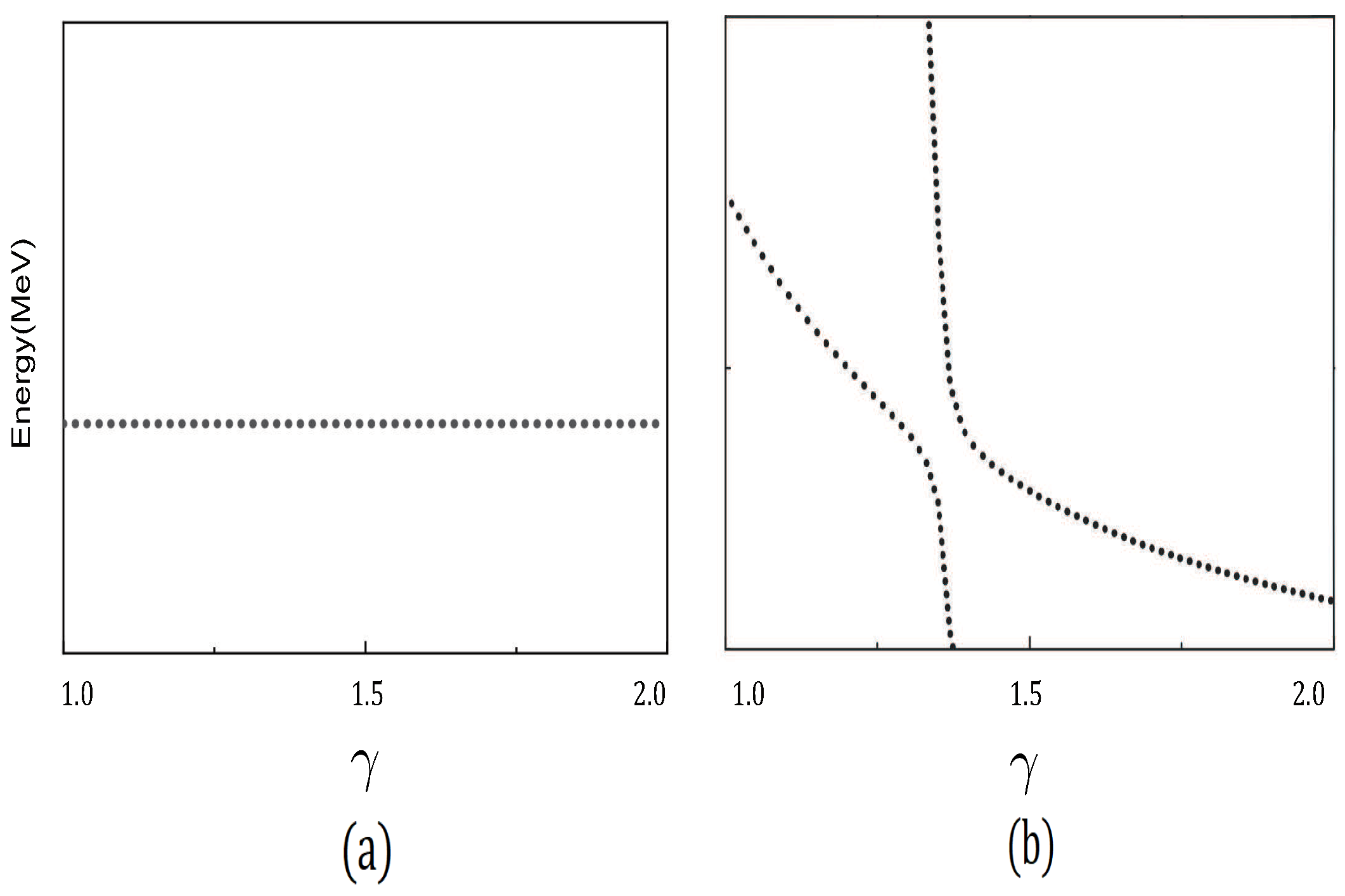
Distinguished from other resonance computation methods based on stabilized eigenvectors, the real-scaling method allows for the direct estimation of decay widths from the stabilization graph. The real-scaling method involves a systematic scaling of the width of Gaussian functions between two groups using a scaling factor, denoted as $\gamma$. This is achieved by simultaneously multiplying all range parameters by a factor, resulting in $R\to \gamma R$. As $\gamma$ increases, the width of the Gaussian functions expands, leading to variations in the system’s intrinsic energy. A stable structure, if present, remains unaffected by the changes in Gaussian function widths. The persistence of this stable structure is visually represented in the real-scaling diagram, thus giving rise to the nomenclature “real-scaling method”. In this approach, false resonant states, reproduced by superabundant colorful subclusters (molecular hidden-color state or diquark structure), fall down to the corresponding threshold. Genuine resonances, on the other hand, persist after coupling to the scattering states and remain stable as $\gamma$ increases. Genuine resonances manifest in two distinct forms:

(1)

Weak coupling: If the energy of a scattering state significantly differs from that of the resonance, indicating weak or no coupling between the resonances and scattering states, the resonance appears as a stable straight line, as shown in Figure 1a.

(2)

Strong coupling: When the energy of a scattering state approaches that of the resonance, indicating strong coupling, an avoid-crossing structure manifests between two declining lines, as shown in Figure 1b.

The decay width can be estimated from the slopes of the resonance and scattering states using Equation (16), where $Slop{e}_r$ denotes the slope of the resonance, $Slop{e}_s$ denotes the slope of the scattering state, and ${\gamma }_c$ represents the energy level difference between the resonance and the scattering state. Furthermore, as $\gamma$ increases continually, the avoid-crossing structure repeats, providing valuable insights into the resonance behavior.

$$\mathrm{\Gamma }=4|V\left({\gamma }_c\right)|\frac{\sqrt{|Slop{e}_r\left|\right|Slop{e}_s|}}{|Slop{e}_r-Slop{e}_s|}$$

(16)

4. Results and Discussions

In this section, we present the numerical results obtained from our calculations, with a primary focus on the quest for potential resonance states within the $s\overline{s}s\overline{s}$ system possessing positive parity. As an initial step in our investigation, we conduct a dynamic calculation utilizing the GEM to ascertain the presence of any bound states. By analyzing the energy levels of the diquark and color-octet structure, we aim to determine the potential for resonance states within the system. Subsequently, after extracting the energies through the generalized eigen-equation, we apply the real-scaling method to verify the stability of the computed energy levels. This methodology enables us to confirm whether the obtained energy levels indeed correspond to stable states.

4.1. Tetraquark States Analysis and Resonance Identification

In this subsection, we present a comprehensive analysis of all conceivable $s\overline{s}s\overline{s}$ tetraquark states with positive parity. The details of these states are summarized in

Table 2. The energies of the $s\overline{s}s\overline{s}$ system. $R_i{F}_j{S}_k{C}_n$ stand for the index of flavor, spin, and color wave functions, respectively. $E_{th}$ means the threshold of the corresponding channel, $E_{sc}$ is the energy of every single channel, $E_{cc}$ shows the energy by channel coupling of one certain configuration, and $E_{mix}$ is the lowest energy of the system by coupling all channels of both configurations (unit: MeV/$c^2$).

${\mathit{J}}^{\mathit{P}}$	$|{\mathit{R}}_{\mathit{i}}{\mathit{F}}_{\mathit{j}}{\mathit{S}}_{\mathit{k}}{\mathit{C}}_{\mathit{n}}\rangle$	Channel	${\mathit{E}}_{\mathit{th}}$	${\mathit{E}}_{\mathit{sc}}$	${\mathit{E}}_{\mathit{cc}}$	${\mathit{E}}_{\mathit{mix}}$
$0^{+}$	$|1111\rangle$	${\eta }^{\prime }{\eta }^{\prime }$	1648	1648	1648	1648
	$|1121\rangle$	$\varphi \varphi$	2031	2032
	$|1112\rangle$	${\left[{\eta }^{\prime }\right]}_8{\left[{\eta }^{\prime }\right]}_8$		2324	2072
	$|1122\rangle$	${\left[\varphi \right]}_8{\left[\varphi \right]}_8$		2255
	$|2214\rangle$	${\left[ss\right]}_6^0{\left[\overline{s}\overline{s}\right]}_{\overline{6}}^0$		2298
	$|2223\rangle$	${\left[ss\right]}_3^1{\left[\overline{s}\overline{s}\right]}_{\overline{3}}^1$		2315
$1^{+}$	$|1131\rangle$	${\eta }^{\prime }\varphi$	1840	1841	1841	1840
	$|1141\rangle$	$\varphi {\eta }^{\prime }$	1840	1841
	$|1132\rangle$	${\left[{\eta }^{\prime }\right]}_8{\left[\varphi \right]}_8$		2247	2199
	$|1142\rangle$	${\left[\varphi \right]}_8{\left[{\eta }^{\prime }\right]}_8$		2247
	$|2253\rangle$	${\left[ss\right]}_3^1{\left[\overline{s}\overline{s}\right]}_{\overline{3}}^1$		2315
$2^{+}$	$|1161\rangle$	$\varphi \varphi$	2031	2032	1648	2031
	$|1162\rangle$	${\left[\varphi \right]}_8{\left[\varphi \right]}_8$		2272	2242
	$|2263\rangle$	${\left[ss\right]}_3^1{\left[\overline{s}\overline{s}\right]}_{\overline{3}}^1$		2315

, which includes the indices of orbit, flavor, spin, and color wave functions for each channel. Additionally, the table provides information on the energy, threshold, and binding energy for each physical channel. Our analysis focuses on rigorously assessing the binding energy ($E_B$) of each color-singlet state by comparing its theoretical calculated value with its corresponding threshold value ($E_B=E_{th}-E$). If $E_B$ is less than 0, we will manually set it to 0. It is noteworthy that color-excited states (color-octet and diquark structure) inherently possess internal attraction due to color interactions, so we omit the $E_B$ values for the color-excited structures. Subsequently, we employ the real-scaling method to investigate whether states displaying attractive interactions, encompassing both color-excited and color-singlet states with $E_B$ values less than zero, can indeed form resonance states. Since we are only interested in the resonant states below 3 GeV/$c^2$, resonance states with energies higher than 3 GeV/$c^2$ are not considered.

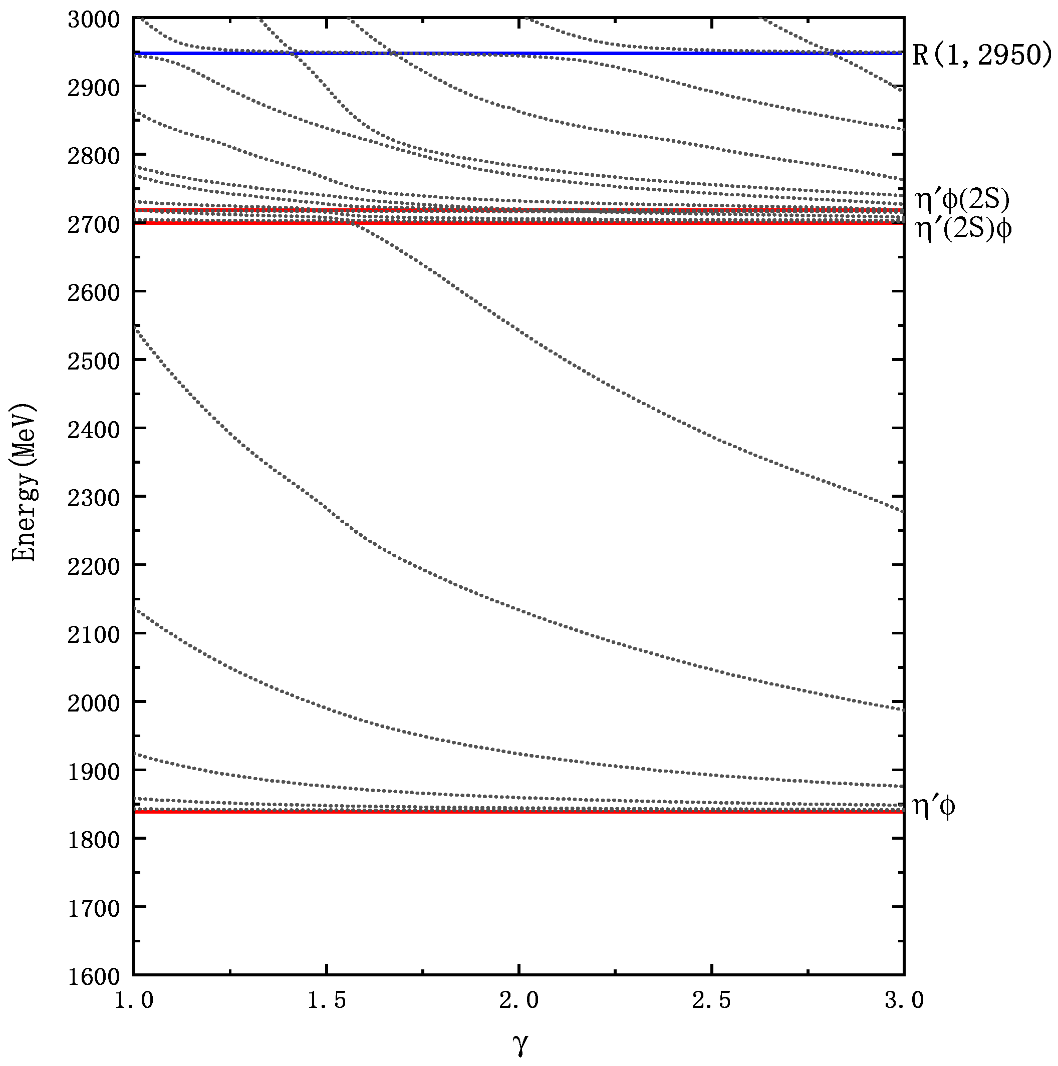
The $J^P=0^{+}$ sector: From the detailed analysis presented in Table 2, we observe a total of two color-singlet states, ${\eta }^{\prime }{\eta }^{\prime }$ and $\varphi \varphi$, existing in the $0^{+}$ system. Additionally, their corresponding color-octet states and two diquark states are identified within an energy range of approximately 2.25–2.32 GeV/$c^2$. Remarkably, the result reveals that the color-singlet states (${\eta }^{\prime }{\eta }^{\prime }$ and $\varphi \varphi$) do not form bound states, even if the channel coupling effect is taken into consideration. To further investigate and identify resonant states, we perform structure-coupling calculations, coupling the color excitation structure with the color-singlet structure using the real-scaling method. The results demonstrate a continuous decrease in energy as the factor $\gamma$ increases from its initial value of 1, which can be found in Figure 2. At approximately $\gamma =1.4$, a distinct avoid-crossing structure emerges, repeating at $\gamma =2.7$, which represents the resonant state in our study. We denote it as $R(0,2150)$ (we label the resulting resonant state with $R(J,energy)$). Analogously, we identify another resonance state, $R(0,2915)$, positioned above the $\varphi \varphi \left(2S\right)$ energy level.

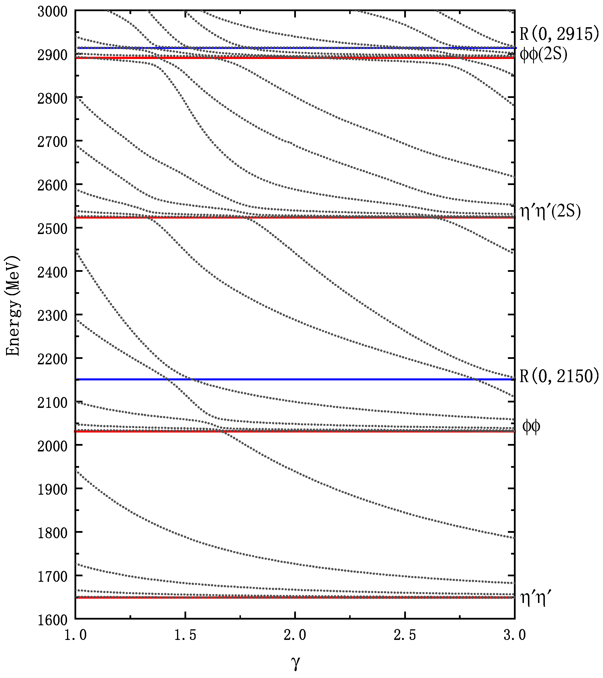
The $J^P=1^{+}$ sector: In principle, a tetraquark system with a total spin of 1 should exhibit three possible combinations: $0\times 1$, $1\times 0$, and $1\times 1$. These combinations, when combined with two types of spatial wave functions ($|R_1\rangle$, $|R_2\rangle$) and four types of color wave functions ($|C_1\rangle$, $|C_2\rangle$, $|C_3\rangle$, $|C_4\rangle$), result in a total of 12 channels for the wave function. However, due to symmetry constraints, the $s\overline{s}s\overline{s}$ tetraquark system with $1^{+}$ spin is limited to only five channels: two color-singlet states (${\eta }^{\prime }\varphi$, $\varphi {\eta }^{\prime }$), two corresponding color-octet states, and one diquark state. Our calculation results indicate that the $s\overline{s}s\overline{s}$ tetraquark system with $1^{+}$ does not have any bound states. The energies of the color-excited structure are predominantly centered around 2.25 GeV/$c^2$. The evident coupling effect among these states is noteworthy, leading to a notable reduction in the minimum energy from 2.25 GeV/$c^2$ to 2.20 GeV/$c^2$ due to the influence of coupling channels. This state may be a potential candidate for $X\left(2100\right)$ in experimental observations. However, within the real-scaling framework, this state undergoes decay to the corresponding threshold, implying its non-existence in our study. Intriguingly, we have identified a stable structure at approximately 2.95 GeV/$c^2$, denoted as $R(1,2950)$, shown in Figure 3.

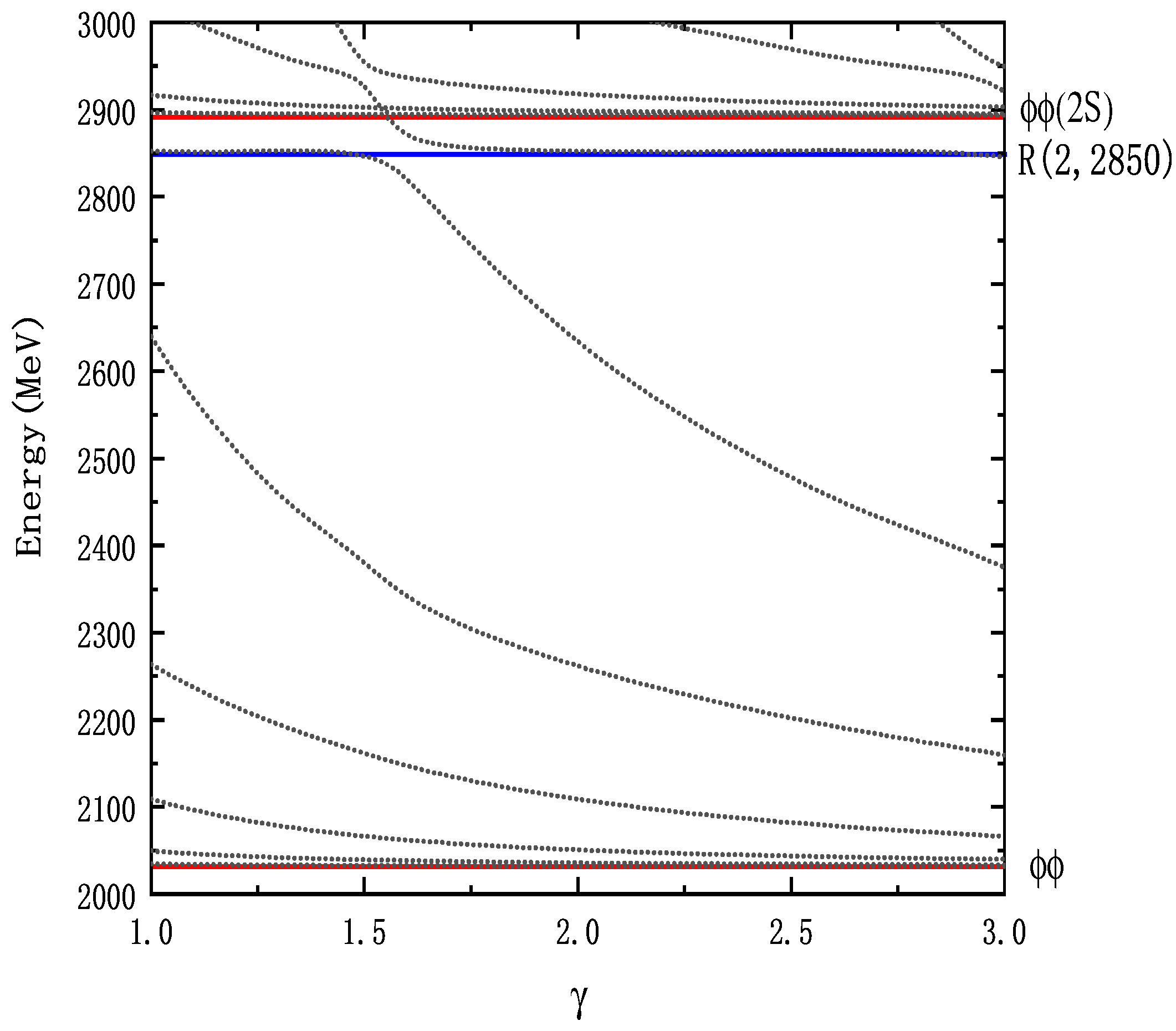
The $J^P=2^{+}$ sector: For a tetraquark system with a total spin of 2, the available states are considerably reduced. In this scenario, there exists only one color-singlet state, $\varphi \varphi$. Additionally, a color-octet molecular state ${\left[\varphi \right]}_8{\left[\varphi \right]}_8$ and a diquark state ${\left[ss\right]}_3^1{\left[\overline{s}\overline{s}\right]}_{\overline{3}}^1$ are present, yielding a total of three wave functions. The energies of these states are primarily concentrated in the range of 2 GeV/$c^2$ to 2.3 GeV/$c^2$. Intriguingly, resonance state calculations reveal a prominent resonance state, $R(2,2850)$, as depicted in Figure 4.

From the comprehensive analysis discussed above, a total of four resonance states are identified: $R(0,2150)$, $R(0,2915)$, $R(1,2950)$, and $R(2,2850)$. These resonance states exhibit a root-mean-square distance concentrated around 1 fm and widths in the range of 40–90 MeV/$c^2$. This can be attributed to their predominant composition of diquark and color-octet states. Of particular interest is that $R(0,2915)$ and $R(1,2950)$ have energies slightly above the $\varphi \varphi \left(2S\right)$ threshold, resembling the characteristics of $X\left(6900\right)$, which resides just above the $J/\psi J/\psi \left(2S\right)$ threshold. This similarity suggests a possible kinship, positioning $R(0,2915)$ and $R(1,2950)$ as potential counterparts to $X\left(6900\right)$. Similarly, the energy of $R(0,2150)$ falls above $\varphi \varphi$ and below ${\eta }^{\prime }{\eta }^{\prime }\left(2S\right)$, resembling the energy characteristics of $X\left(6600\right)$. This observation leads to the hypothesis that $R(0,2150)$ could be a kin to $X\left(6600\right)$. On the other hand, $R(0,2150)$ could also be a candidate for $f_0\left(2100\right)$.

4.2. Comparison with the Other Works

As highlighted in our introduction, there has been some prior research on the $s\overline{s}s\overline{s}$ tetraquark system. This diverse body of work, encompassing various models and methods, not only checks the model dependence of the results but also contributes to a more profound comprehension of the $s\overline{s}s\overline{s}$ tetraquark system’s nature. These research endeavors broadly fall into two categories: QCD sum rule and quark potential energy models. Our findings, as presented in

Table 3. The comparison of the energies of resonances in $s\overline{s}s\overline{s}$ systems with positive parity in different calculations (unit: MeV/$c^2$).

State	Ref. [19]	Ref. [21]	Ref. [20]	Ref. [23]	Ref. [22]
$J^P=0^{+}$
$R(0,2150)$	1925	${2110}_{-21}^{+19}$	${2450}_{-24}^{+20}$	2218	-
$R(0,2915)$				2440
				2781
				2876
				2948
				3232
$J^P=1^{+}$
$R(1,2950)$	-	${2060}_{-20}^{+18}$	-	2323	$2080\pm 12$
				2867
				2954
$J^P=2^{+}$
$R(2,2850)$	-	${2090}_{-22}^{+19}$	${3070}_{-33}^{+25}$	2378	-
				2878
				2963
				2977

, demonstrate qualitative consistency with previous calculations. For a quantum number of $0^{+}$, our calculations yield two resonant states, namely, $R(0,2150)$ and $R(0,2915)$. Remarkably, the energy of $R(0,2150)$ closely resembles the energy values reported in other studies. In Ref. [23], up to six energy levels are presented, one of which closely matches our $R(0,2915)$ energy value. Notably, the remaining potential energy levels between $R(0,2150)$ and $R(0,2915)$ in our calculations are found to decay into their corresponding threshold states, resulting in the identification of two resonance states. At a quantum number of $1^{+}$, both QCD sum rule methods yield energies approximately around 2060 MeV/$c^2$ [21,22], which is notably lower than the energy associated with $R(1,2950)$ in our findings. In fact, in our model’s calculations, the energy of the diquark structure also falls in the vicinity of 2200 MeV/$c^2$. However, it is important to note that strong channel coupling effects in our calculations lead to the decay of some energy levels into their respective threshold channels. On the other hand, the energy level of 2954 MeV/$c^2$ in Ref. [23] closely corresponds to our result, $R(1,2950)$. In the case of a quantum number of $2^{+}$, our energy level calculations exhibit significant similarities to the $1^{+}$ quantum number scenario. The energy value associated with $R(2,2850)$ is in strong agreement with results reported in Refs. [20,23].

5. Summary

Within the framework of the quark model, we conducted a comprehensive study on the $s\overline{s}s\overline{s}$ system, exploring three different quantum number combinations, namely, $J^P=0^{+}$, $1^{+}$, and $2^{+}$. Our investigations include not only the diquark structure but also molecular structures, while accounting for all permissible color, flavor, and spin configurations.

The dynamic calculations yielded no bound states under any of the three quantum numbers. Nevertheless, the presence of color attraction mechanisms within the color-excited structures, encompassing both color-octet structures and diquark structures, introduced the possibility of several potential resonances. To ascertain the stability of these potential resonant states, we employed the real-scaling method. The results revealed that the majority of false resonances decayed into their corresponding threshold channels, leaving behind only four confirmed resonance states: two $J^P=0^{+}$ resonances $R(0,2150)$, $R(0,2915)$, one $J^P=1^{+}$ resonance $R(1,2950)$, and one $J^P=2^{+}$ resonance $R(2,2850)$. These four resonant states share similar compositions, primarily dominated by diquark structures and color-octet structures. Consequently, they exhibit root-mean-square distances of around 1 fm and widths within the range of 40–90 MeV/$c^2$, as depicted in

Table 4. The main component, width, and root-mean-square distances of resonances in $s\overline{s}s\overline{s}$ systems.

State	Main Component	Width (MeV/${\mathit{c}}^2$)	${\mathit{r}}_{\mathit{s}\overline{\mathit{s}}}\left(\mathit{fm}\right)$	${\mathit{r}}_{\mathit{ss}}\left(\mathit{fm}\right)$	${\mathit{r}}_{\overline{\mathit{s}}\overline{\mathit{s}}}\left(\mathit{fm}\right)$
$J^P=0^{+}$
$R(0,2150)$	diquark structure($48\%$)+color-octet($50\%$)+color-singlet($2\%$).	65	0.87	0.94	0.94
$R(0,2915)$	diquark structure($45\%$)+color-octet($51\%$)+color-singlet($4\%$).	45	0.98	1.11	1.26
$J^P=1^{+}$
$R(1,2950)$	diquark structure($41\%$)+color-octet($52\%$)+color-singlet($7\%$).	85	1.06	0.96	0.96
$J^P=2^{+}$
$R(2,2850)$	diquark structure($51\%$)+color-octet($48\%$)+color-singlet($1\%$).	90	1.01	0.77	0.77

.

Based on our result, the resonance $R(0,2150)$ emerges as a plausible candidate for the $f_0\left(2100\right)$ meson. It is noteworthy that the resonance $R(0,2915)$ is positioned above the decay threshold for $\varphi \left(2S\right)\varphi$. A parallel can be drawn with the observed state $X\left(6900\right)$, which similarly lies just beyond the $\psi \left(2S\right)J/\psi$ threshold. Despite the detection of $X\left(6900\right)$ within the $J/\psi J/\psi$ invariant mass distribution, we advocate for future experimental investigations to extend their search to the invariant mass spectrum of $\psi \left(2S\right)J/\psi$.