Abstract
Genetic algorithms are a powerful tool in optimization for single and multimodal functions. This paper provides an overview of their fundamentals with some analytical examples. In addition, we explore how they can be used as a parameter estimation tool in cosmological models to maximize the likelihood function, complementing the analysis with the traditional Markov chain Monte Carlo methods. We analyze that genetic algorithms provide fast estimates by focusing on maximizing the likelihood function, although they cannot provide confidence regions with the same statistical meaning as Bayesian approaches. Moreover, we show that implementing sharing and niching techniques ensures an effective exploration of the parameter space, even in the presence of local optima, always helping to find the global optima. This approach is invaluable in the cosmological context, where an exhaustive space exploration of parameters is essential. We use dark energy models to exemplify the use of genetic algorithms in cosmological parameter estimation, including a multimodal problem, and we also show how to use the output of a genetic algorithm to obtain derived cosmological functions. This paper concludes that genetic algorithms are a handy tool within cosmological data analysis, without replacing the traditional Bayesian methods but providing different advantages.
1. Introduction
Genetic algorithms (GAs), established for decades, are tools from evolutionary computation [1,2,3,4,5] that solve many function optimization problems. Evolutionary computation is focused on algorithms exploiting randomness to solve search and optimization problems using operations inspired by natural evolution [6]. It includes several methods for stochastic or metaheuristic optimization [7,8]; notable examples are Particle Swarm Optimization (PSO) [9] based on the social behavior of organisms of the same species such as birds, the Giant Trevally Optimizer (GTO) [10,11,12] inspired by the hunting behavior of predatory fish, and Artificial Rabbits Optimization (ARO), drawing inspiration from social interactions among rabbits [13,14]. Within evolutionary computation, the most relevant methods are genetic algorithms [15,16], genetic programming [17], and evolutionary strategies [18]; their success is due to their ability to navigate intricate, non-linear, and high-dimensional search spaces.
In particular, genetic algorithms stand out as powerful tools for optimization problems because they mathematically always guarantee, under certain conditions, to find the best solution. Despite challenges posed by local optimum values [19], this property puts them at an advantage over other techniques. Rooted in the emulation of natural selection and evolution, the iterative process of GAs involves generating a population, subjecting it to fitness-based selection, and applying genetic operators, such as crossover and mutation. This iterative approach drives the evolution of increasingly optimal solutions over generations. GAs thrive in situations with multiple optima, irregular landscapes, or where an analytical solution is difficult to achieve. Its adaptability allows for the simultaneous exploration of numerous candidate solutions, making them effective in various optimization challenges. Unlike traditional optimization methods, GAs have the advantage of not relying on derivatives, providing excellent robustness in high-dimensional or more complex problems. Inspired by natural evolution, these algorithms efficiently explore vast and unknown search spaces [20]. Their ability to solve complex and dynamic projects makes them valuable in diverse fields, including medicine [21,22,23], epidemic dynamical systems [24,25], geotechnics [26], market forecasts [27], and industry [28], among others. A particularly successful application in the Deep Learning era is the optimization of neural networks, which are huge computational models in which genetic algorithms help to find optimal combinations of hyperparameters [29,30,31].
With the accelerated development of computational resources, genetic algorithms and other machine learning algorithms have been exploited in several scientific fields in recent years. Remarkably, they have resulted in significant advances in understanding particle physics [32,33,34], astronomical information [35,36,37,38], and cosmological phenomena [39,40,41,42,43,44].
Genetic programming, another method from evolutionary computation, has been widely used in astrophysics and cosmology [45,46,47,48,49,50], which allows for symbolic regression for a given dataset, treating regression as a search problem to find the best combination of mathematical operators generating an expression fitting the data. Although genetic programming and genetic algorithms solve different tasks, they use similar operators to find solutions. In this work, we focus on genetic algorithms, mentioning genetic programming for reference, assuming the astrophysical community may be more familiar with it. Moreover, genetic algorithms are the most fundamental and successful evolutionary computation technique, and understanding them is useful for studying other evolutionary computation methods, including genetic programming.
On the other hand, parameter estimation in cosmology is a very relevant task that finds a combination of values for parameters describing a cosmological model based on observational data. The goal is to refine theoretical models to align with observations for a more precise understanding of the universe. In cosmological parameter estimation, the most robust and successful algorithms are Markov chain Monte Carlo; however, these methods sometimes are computationally expensive, and recent advancements try to attack this issue with new statistical or machine learning techniques, including the iterative Gaussian emulation method [51], adaptive importance sampling, parallelizable Bayesian algorithms [52], Bayesian inference accelerated with machine learning [53,54,55], or likelihood-free methods [56,57].
This paper aims to achieve two primary objectives: firstly, to provide a comprehensive introduction to genetic algorithms and elucidate their application in cosmological parameter estimation, and secondly, to demonstrate the complementarity of GAs with traditional Bayesian inference methods. We include illustrative examples of optimization problems and their applications in cosmology. Particularly, we delve into using genetic algorithms to constrain the parameter space of dark energy models based on observational data. It is pertinent to mention that GAs cannot perform the same tasks as MCMC methods, and we do not try to replace them; we only perform parameter estimation with GAs by optimizing the likelihood function, whereas MCMC methods sample the posterior probability function. However, we analyze their relevance as an alternative and complementary method, as discussed in Section 4.1.
The structure of this paper is as follows: In Section 2, we present the basics of genetic algorithms and an insight into their functionality. In Section 3, we provide some examples of the optimization of analytical functions by applying genetic algorithms. Section 4.1 describes the path to perform cosmological parameter estimation using these algorithms. Section 4.2 contains examples of multimodal problems in cosmology, and in Section 4.3, we justify how to obtain cosmological-derived parameters from a likelihood optimization. Finally, Section 5 summarizes our final remarks.
2. Fundamentals of Genetic Algorithms
2.1. Biological Fundamentals
Bioinspired computing is a field of computer science based on observing and imitating natural processes and phenomena to develop algorithms and computational systems [58]. These algorithms seek to solve complex problems. The bioinspired computation is classified into three main categories [58]: evolutionary algorithms (such as genetic algorithms), particle swarm intelligence (imitating collective behaviors) [7,59,60,61], and computational ecology (inspired by ecological phenomena) [8,62].
Genetic algorithms solve optimization [1,2,3,4,5] and search problems inspired by fundamental concepts of genetics and evolution [8,63,64]; some of its key points are as follows:
- Natural selection—This is the central principle in the theory of evolution. Just as better-adapted organisms are more likely to survive and reproduce in nature, GAs favor the fittest or most promising solutions from a population of candidate solutions. In nature, over several generations, the most promising characteristics of individuals survive to be inherited by the new generations. This is what genetic algorithms seek to do to have better solutions as more generations pass by.
- Crossing—Also called recombination, it is a process in which genes from two parents are combined to create offspring with characteristics inherited from both parents. GAs apply the idea of crossover by combining partial solutions from two individuals in the population to generate new solutions that can inherit desirable characteristics from both parents.
- Mutation—A mutation is recognized as the stochastic alterations in an organism’s genetic material. In the GAs, a mutation introduces random changes in a small part of the candidate solutions, e.g., it may change the value of a bit, which increases the diversity of possible solutions and improves the exploration of the search space.
- Reproduction and inheritance—In the same sense as in nature, in genetic algorithms, these operations allow for the transmission of some characteristics of the parent solutions to the solutions of the next generation (offspring).
2.2. Genetic Algorithm Operations
John Holland was the first to introduce the genetic algorithm in 1975 in his book Adaptation in Natural and Artificial Systems [3,15]. According to the GA context, a population is a set of possible solutions to a given problem. Each individual has a genotype encoded in bits, which is then expressed as a phenotype in the problem context. The way to encode the possible solutions is fundamental to attacking a problem with GAs, and there are several options to perform it, for example, with binary, integer, or real encoding, among others [65].
Alternatively, assessing an individual’s quality or a potential solution involves employing a metric or target function, which is ideally expected to approach its optimal value in the final generations. For the analogy of natural selection, this target function, or objective function, is called the fitness function. In practice, in GAs, the fitness function is directly the function to be optimized. This is unlike genetic programming, where the fitness function is a measure of the error between the algebraic expression found and the dataset used due to the regression task that genetic programming addresses.
The continuous evaluation of all the individuals (possible solutions) of a population with this fitness function and the applications of genetic operations to produce new generations allow for GAs to find the optimal value of this function. In the following list, we describe the fundamental procedures of genetic algorithms [66]:
- Selection—It is the method of choosing the best solutions to play the role of parents and improve the quality of the offspring. Several selection methods include the roulette [67], random [68], ranking [69], tournament [70], and Boltzmann entropy selections [71].
- Crossover—It is also called recombination, which generates a new possible solution given two previously selected parents. There are several crossover methods, such as one point, two points, N points, uniform, three parents, random, and order. The crossover operation has an associated probability () that determines how many individuals recombine given the population, with indicating that all the products come from the recombination and , meaning they are exact copies of the parents.
- Mutation—After crossover, mutations make it possible to maintain diversity in the population and prevent it from stagnating at the local optima [72]. There are several types of mutation operators, such as flipping a gene if it is in the same position as in the parent; swapping values at random positions; flipping values from left to right, or in a random sequence; and shuffling random positions. Mutation also has a probability associated with it that indicates how likely it is to randomly change a gene (bit) of a possible solution. The mutation value must be low for an efficient search within the genetic algorithm1.
- Replacement—The last step is the replacement, which keeps the population size constant by eliminating individuals after recombination. There are three methods: strong replacement (random), weak replacement (the two fittest), and replacing both parents (the children replace both parents).
- Elitism and Hall-of-Fame—The elitism method ensures that the best individuals are not discarded but transferred directly to the next generation. Hall-of-Fame is an integer that indicates how many individuals are considered under elitism to be retained in the next generation. Elitism is necessary to ensure that genetic algorithms always find the best solution [19]. Elitism and Hall-of-Fame are often considered distinct from the general replacement strategy. While the replacement strategy primarily focuses on selecting individuals for reproduction and forming the next generation, the elitism and Hall-of-Fame mechanisms specifically address preserving the best-performing individuals.
- Stopping criteria—A mechanism is needed to finalize the execution of the genetic algorithm. Some ways to perform it are to stop after a fixed number of generations, after a specific time-lapse, to finish the process if the best fitness does not change for several generations (steady fitness), or to stop it if there are no improvements in the objective function for several consecutive generations (generation stagnation).
In this way, we can summarize that genetic algorithms are a process that involves some crucial steps: the initialization of a population form of solutions, selection of parents according to their fitness, recombination of genes by crossing, introduction of variability by mutation, substitution of individuals, and running the algorithm until the stopping criterion is satisfied. The operations described above are repeated within a loop, generation after generation, until a satisfactory solution or convergence criterion is reached.
2.3. Schema Theorem
The heuristic search of genetic algorithms is based on Holland’s schema theorem, which states that the chromosomes have patterns called schemas. This schema theorem deals with the decomposition of chromosomes into schemas and their influence on the evolutionary dynamics of the population.
A schema is a binary string of fixed length representing a chromosome pattern. For example, in a chromosome of length 6, the schema 001X00 defines a string that starts with 001, has an unknown bit X, and ends with 00.
The fitness of a schema refers to how many individuals in the population contain that specific schema. It can be represented as a fitness function that denotes the fitness of the schema S.
The schema theorem states that high-fitness schemas are more prevalent in future generations. This is because schemas with high fitness are more likely to be selected and recombined, leading to population improvement in terms of fitness. Mathematically, we can express this as:
where is the fitness of the schema S at the next generation , is the fitness of the schema S in the current generation , and finally, is the mutation probability.
This equation indicates that the fitness of the schema in the next generation is at least equal to the current fitness, modulated by the mutation probability. If is low, schemas with high fitness will likely survive and propagate in future generations, contributing to population improvement.
3. Genetic Algorithm Application
In this section, we implement a genetic algorithm to optimize univariate functions and extend its application to higher-dimensional problems. The general structure of a genetic algorithm is provided in the Algorithm 1.
| Algorithm 1 Simple Genetic Algorithm |
Parents ← {randomly generated population} While not (termination) Calculate the fitness of each parent in the population Children while |Children| < |Parents| Use fitness to probabilistically select a pair of parents for mating Mate the parents to create children and Children ← Children Loop Randomly mutate some of the children Parents ← Children Next generation |
Several libraries incorporate genetic algorithms, such as Distributed Evolutionary Algorithms (DEAP) [73], Karoo GP [74], Tiny Genetic Programming [75], and Symbiotic Bid-Based GP [76]. These libraries simplify the implementation of genetic algorithms. In this paper, we have utilized the DEAP library, which boasts comprehensive documentation.
3.1. Single Variable Functions
Considering the following three functions, we aim to use a custom genetic algorithm to find their global maxima:
- ;
- ;
- .
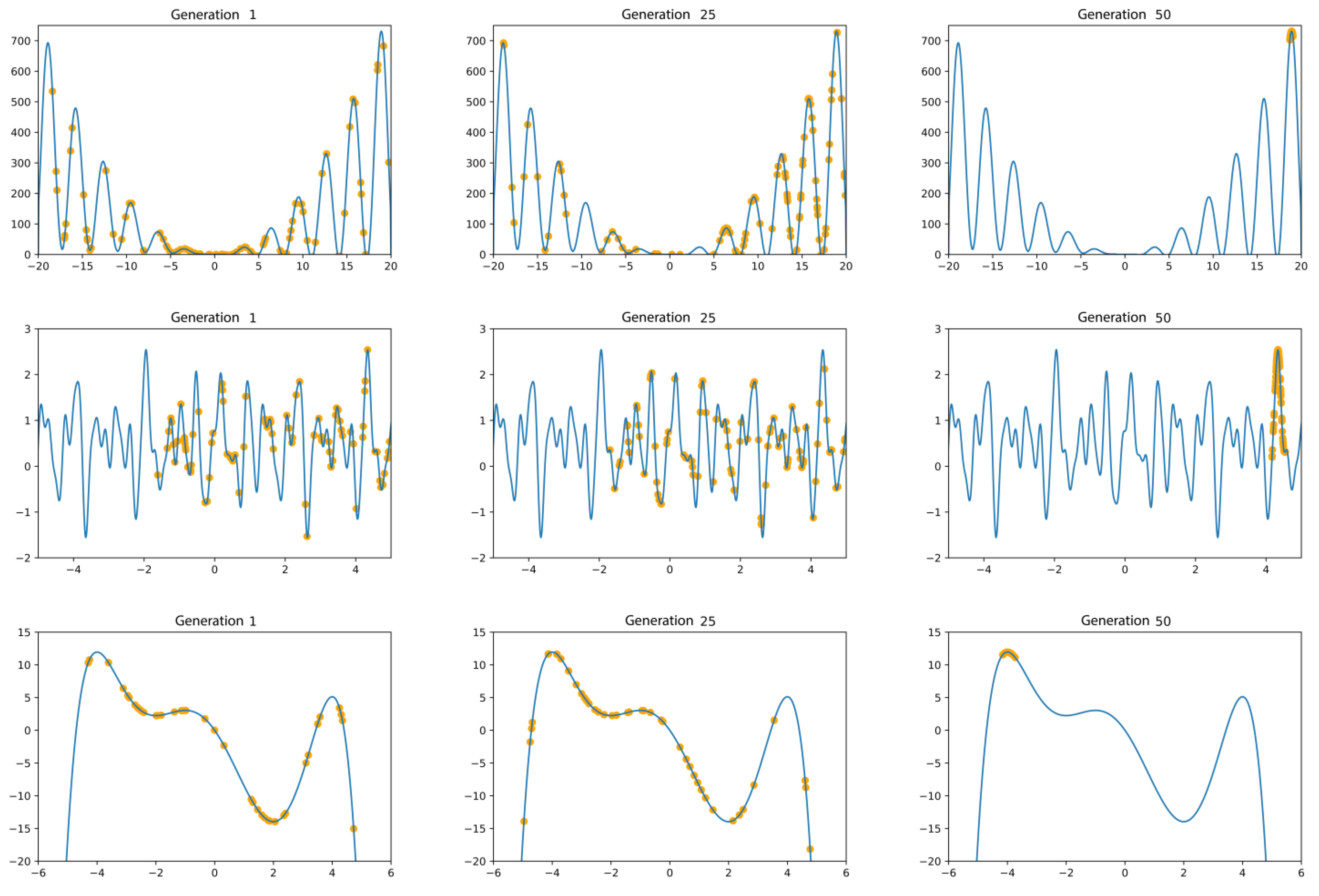
In Figure 1, it can be seen how the above functions are optimized by a genetic algorithm, using a population size of 100 individuals, with a Hall-of-Fame size equal to 1, a mutation probability of 0.2, and a crossover probability of 0.5, over 50 generations. Note that as the generations progress, the individuals are closer to the global maxima. Another interesting feature is that, despite the local optima, the genetic algorithm in all the functions can find the global optima, as it is mentioned in the Introduction and Ref. [19].
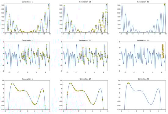
Figure 1.
The search space exploration is presented for three different generations: 1, 25, and 50. As we advance through the generations, a greater concentration of individuals (yellow dots) is seen at the global maxima. In the top panels, . In the central panels, . In the bottom panels, .
3.2. Multimodal Functions
Genetic algorithms can also address problems with multiple dimensions and maxima by modifying the representation of candidate solutions and the operators used to generate new solutions. They can explore complex search spaces efficiently and identify global or local optima by appropriately designing crossover and mutation operators and analyzing different encoding techniques.
We use the Himmelblau function to demonstrate how genetic algorithms can be used to optimize these types of multimodal functions. We use the DEAP library, a robust Python framework for evolutionary computation, to achieve our goal. The following equation defines Himmelblau’s function:
The niching and sharing technique is employed to identify all the global optima within a single genetic algorithm run. This concept draws inspiration from nature, where regions are divided into sub-environments or niches, enhancing population efficiency and survival. Individuals compete for resources in these niches independently of those in other niches. By integrating a sharing mechanism into the genetic algorithm, individuals are incentivized to explore new niches, discovering multiple optimal solutions, each considered as a niche. Typically, this is achieved by dividing an individual’s fitness value by the sum of distances from all other individuals. This approach penalizes overpopulated niches by distributing the local rewards among their individuals [77].
Niching involves dividing the population into subpopulations, each assigned to explore a specific region in the solution space. This encourages diversity by allowing genetically engineered individuals to compete for fitness locally. Conversely, sharing ensures a fair distribution of the fitness resources among individuals within the same niche. An individual’s fitness is influenced not only by its performance but also by the performance of its neighbors, preventing overemphasis on a specific region and promoting a balanced exploration. This approach prevents premature convergence to a local maximum, allowing for the simultaneous exploration of different regions and ultimately facilitating the identification of the global maximum. Applying this technique effectively requires a larger population size and more generations than a simple genetic algorithm. This is essential to spread the population across the sample space, targeting different niches and, consequently, identifying multiple optimal maxima. In our experiment, we executed the algorithm with 200 individuals and 200 generations, and the outcomes are summarised in Figure 2 and Table 1.
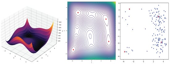
Figure 2.
On the left panel, we have Himmelblau’s function, while the center panel displays its contour diagram. The red points on the contours represent the global minima of the function. On the right panel, we can observe the application of the genetic algorithm with niching and sharing, specifically for Himmelblau’s function, the blue dots are individuals and the red dots represent the best solutions.

Table 1.
A comparison is made among the four real global optima of Himmelblau’s function [77] and those found by the genetic algorithm using niching and sharing.
As can be seen in Table 1, these results are remarkably similar to the real values. Improving these results is possible by increasing the number of individuals and generations. It should also be noted that this technique is not limited to three dimensions but can be generalized to N dimensions and can support the search for global M optima. However, it is important to remember that as the number of dimensions increases, more computational resources are required to search effectively.
3.3. Statistical Analysis
Genetic algorithms are handy tools in statistical applications for optimizing likelihood functions, thereby determining the parameters of a scientific model (which is precisely what this article aims to demonstrate). However, reporting a confidence interval for the output of a genetic algorithm can be more complex than in classical statistical methods. The most rigorous technique relies on having a mathematical model of the genetic algorithm’s convergence that extends beyond Holland’s schema theory for the simple genetic algorithm published in 1975.
Because the state of the population in a genetic algorithm depends solely on the previous state in a probabilistic manner, Markov chains have been studied as suitable models for specific applications, and more recently, others have been modeled as martingales [78,79].
However, it is possible to resort to less rigorous techniques. One approach is to assume a distribution for the optimized parameters. For instance, assuming the parameters follow a normal distribution, the confidence interval can be calculated based on standard deviations, and the confidence ellipses can be computed using Fisher matrices. This is the procedure employed in this article. Another procedure involves using the Bootstrap method or other re-sampling techniques [80].
4. Application in Cosmology
In observational cosmology, one of the fundamental tasks is to determine the values of the free parameters for a given theoretical model based on observational measurements. This involves creating a function that captures the discrepancies between observed data and theoretical predictions and using it to obtain a parameter estimate that fits the data well. The likelihood function is typically used to represent the data’s conditional probability given the theory and its parameters. Although Bayesian inference is the most robust method for parameter estimation in cosmology, as it allows for sampling the posterior probability of parameters given the data, it can be computationally intensive (see the nomenclature under the Bayesian formalism of Bayes’ theorem [81,82]); instead of sampling the posterior probability function to estimate parameter values efficiently, optimization algorithms can be used to find the maximum likelihood function. In Reference [82], there is an exciting overview of the difference between sampling and optimization, and it can be seen that they are two different tasks that can be complementary. This section presents three applications that show how genetic algorithms can be applied to analyze cosmological data. First, we offer parameter estimation in three cosmological models: CDM, CPL, and PolyCDM. We then discuss how genetic algorithms can be used in a cosmological model with multiple maximum values, such as the graduated dark energy model presented in Ref. [83].
The datasets utilized in this section comprise 31 cosmic chronometers [84,85,86,87,88,89,90,91], Baryon Acoustic Oscillation measurements (BAO) [92,93,94,95,96,97], 1048 Type Ia supernovae (SNeIa) sourced from the Pantheon compilation [98], and binned data from the Joint Light Analysis SNeIa compilation [99].
Considering the datasets mentioned above, we employ the following log-likelihood functions for the Bayesian inference and optimization methods:
where the index i ranges from 1 to 3, corresponding to the three datasets: cosmic chronometers [] and BAO [], where represents the Hubble, volume averaged, and angular distance; and SNeIa [], where denotes the distance modulus. In this context, represents the observed measurements, while represents the theoretical values for the cosmological models. The matrices encompass the covariance information, accounting for systematic and statistical errors.
We implemented a module to work with the DEAP genetic algorithms within the SimpleMC2 code for our cosmological parameter estimation [100]. In some of the subsequent results, we compare the genetic algorithm’s outcomes with those of Bayesian inference obtained using the nested sampling algorithms, a specialized type of Markov chain Monte Carlo (MCMC) technique [81,101]. Additionally, we utilize the Fisher matrix formalism described in Refs. [102,103] to calculate the confidence intervals and generate error plots for the genetic algorithm-based parameter estimation. It is important to emphasize that genetic algorithms are not employed to generate posterior samples; instead, they are used to explore maximum likelihood estimation, which can yield similar and quicker results than parameter estimation. However, they cannot replace the robustness of MCMC methods. Furthermore, we conducted maximum likelihood estimation using a classical optimization method, specifically the L-BFGS algorithm [104], for comparison purposes and to assess the advantages of genetic algorithms.
4.1. Cosmological Parameter Estimation
As previously mentioned, we employ genetic algorithms to evaluate their effectiveness in parameter estimation. As a proof of the concept, and for simplicity, we consider three cosmological models, CDM, CPL, and PolyCDM, which are described below:
- CDM. The CDM model serves as the standard cosmological model and comprises two primary components: cold dark matter (CDM), which plays a pivotal role in the universe’s structure formation, and dark energy, which exhibits a counter-gravitational behavior, leading to the universe’s accelerated expansion. The cosmological constant, denoted by , is the simplest and most straightforward representation of dark energy, which exerts a pressure equal in magnitude but opposite in sign to the universe’s energy density (). For a flat universe in the late stages of its evolution, the equation governing its expansion is given by , where a represents the scale factor, the dot denotes the derivative with respect to time, signifies the density of dark matter and baryons, and accounts for the dark energy content in the form of a cosmological constant. These two parameters describe the evolution of the universe’s content. Incorporating their initial conditions denoted with a subscript 0, this equation can be re-expressed in terms of the redshift as follows:where denotes the Hubble constant, providing the present rate of expansion of the universe. The parameters and are specific to the CDM model. The former represents the current dimensionless density of dark matter (plus baryons), while the latter signifies the dimensionless density of dark energy. These parameters are subject to the constraint ; when this equality holds, we have a flat universe [105]. Consequently, for this model, we effectively have two free parameters, namely, h and , which we simplify by denoting as for brevity.
- CPL model. One can discern dark energy’s characteristics by investigating its state equation, denoted as , where p and represent the pressure and dark energy density, respectively [106]. Chevallier, Polarski, and Linder introduced the following parametrization for the equation of state, , where signifies the current value of the equation of state. In contrast, represents its rate of change over time [106]. This equation of state leads to the following derivation:Now, the parameter estimation consists of finding the free parameters , , and and .
- PolyCDM. We can consider an extension of dynamical dark energy by introducing spatial curvature, , which adapts to the evolution of dark energy at low redshifts [41]. By performing a Taylor series expansion of the Equation (4) [107], we arrive at the PolyCDM model:where represents the dark matter; and baryon, contribution, and can be interpreted as the “lost matter” [107]. PolyCDM can be considered a parametrization of the Hubble parameter [108].
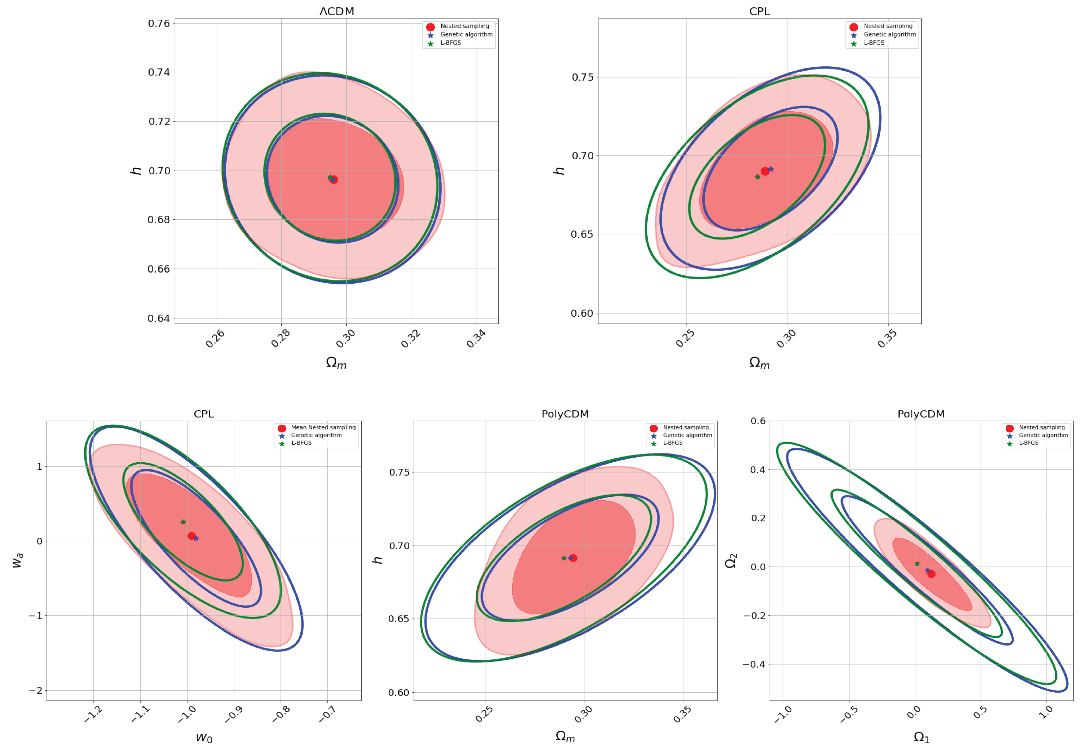
For all the models mentioned above, we use a genetic algorithm with elitism, using 50 generations, a mutation probability of 0.2, a crossover probability of 0.7, a population comprising 100 individuals, and a Hall-of-Fame size of 2 to maximize the likelihood probability function. Table 2 and Figure 3 present the parameter estimation results obtained throughout the three methods outlined earlier. It is noticeable that, in most cases, the genetic algorithm results closely align with the parameter estimations derived from the nested sampling. Consequently, although they are slower than optimization methods like the L-BFGS method, genetic algorithms offer greater precision while remaining faster than MCMC algorithms. It is important to note that genetic algorithms maximize the likelihood function rather than sampling the posterior distribution. This distinction can be computationally advantageous compared to Bayesian inference procedures in specific scenarios. However, GAs lack the assignment of weights to individuals, as found in Bayesian inference samples, and their exploration of parameter space differs from MCMC methods, which rely on Markov chains and probabilistic conditions. Genetic algorithms, instead, focus on achieving improved solutions in each generation.
Table 2.
Parameter estimation via genetic algorithms for the CDM, CPL, and PolyCDM models utilizing cosmic chronometers, BAO, and SNeIa datasets. The value represents the optimal fitness value.
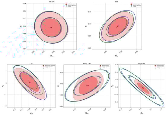
Figure 3.
Two-dimensional posterior distribution plots showing the parameter mean estimates from nested sampling and the parameter values obtained through likelihood maximization using the L-BFGS and genetic algorithm methods (see color labels). Note that the confidence intervals are different due to their nature: optimization methods that maximize the likelihood function (L-BFGS and genetic algorithms) make use of the Fisher matrix formalism to approximate the errors (see Section 3.3), while the MCMC (nested sampling) method constructs its confidence intervals from sampling the posterior probability function. In the nested sampling results, the darker red regions represent , and the lighter red regions represent .
4.2. Multimodal Models
Parameter inference in some models can lead to the identification of multiple optima, meaning that posterior probability functions can have multimodal distributions. To address this complexity, Bayesian nested inference algorithms, such as multinest [109], are a sampling method designed to deal with multimodal distributions, allowing for the effective sampling of the parameter space. In contrast, classical optimization algorithms are limited to finding a single maximum. Genetic algorithms, thanks to niche and sharing techniques (see Section 3.2), have the ability to exhaustively explore the parameter space, even in the presence of local maxima. An example of a model with multiple maxima in its posterior distribution is the case of graduated dark energy [83], which is governed by the following Friedmann equation:
where is the dimensionless density parameter of the dark energy with and . Also, is defined in terms of and another parameter in the following way: . One maximum value corresponds to the CDM model, whereas the other is present to alleviate the Hubble tension. This model resembles a rapid transition of the universe from anti-de Sitter vacua to de Sitter vacua; see the details of the model in the references [83,110,111,112,113].
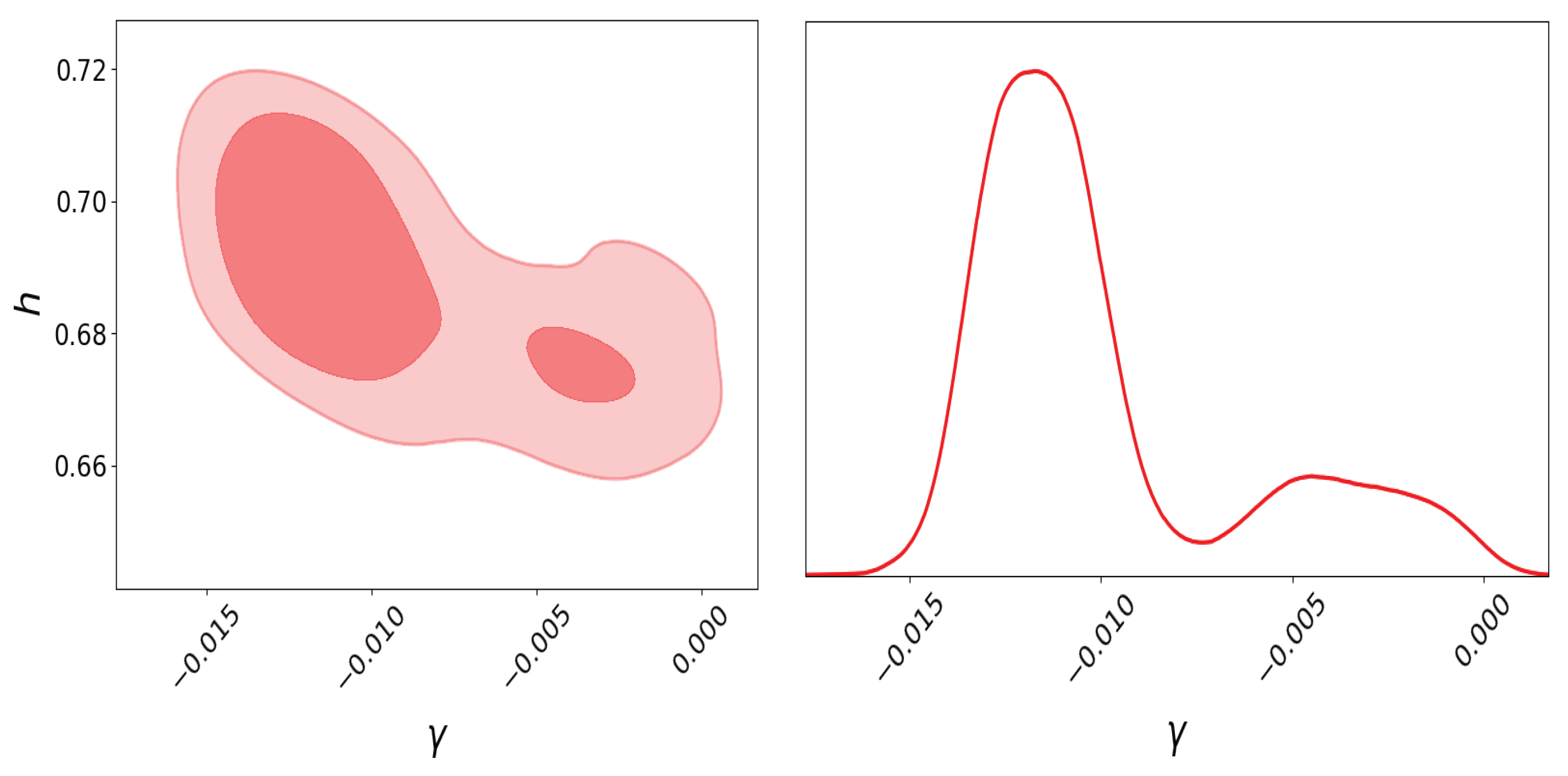
For the genetic algorithm with elitism used in this case, we set 20 generations, 200 individuals for the population, crossover and mutation probabilities of 0.5 and 0.2, respectively, and a Hall-of-Fame of size 2. Therefore, the free parameters for the graduated dark energy model are , , , and . For this example, to appreciate the multimodality in the graduated DE model, we use the same data as that in the original work (Ref. [83]), i.e., cosmic chronometers, BAO, and SNeIa (binned data from the Joint Light Analysis compilation [99]), but for simplicity, we do not use the Planck information. We also fix . Performing Bayesian inference on this model, the posterior distribution for the parameter is shown in Figure 4, in which two modes exist. In Table 3, we can analyze the outputs of the parameter estimation using nested sampling through posterior distribution sampling, the L-BFGS optimization method, and a genetic algorithm maximizing the likelihood distribution function; we can notice that the results maximizing the likelihoods are roughly consistent with the parameter estimation with Bayesian inference; however, for the value, the L-BFGS method is unable to find a value different to zero, and it is far from the estimation of this parameter using the same data.

Figure 4.
Posterior plots with nested sampling for h and parameters of the graduated DE model using HD + BAO + SN, where the bi-modality is shown. Left: Two-dimensional posterior plot for h vs. . The darker red region represents , and the lighter red region represents . Right: One-dimensional posterior distribution plot for parameter.
Table 3.
Parameter estimation with nested sampling (sampling the posterior probability distribution function), L-BFGS, and genetic algorithm. In these cases, we only consider the maximum likelihood found in the three methods and their corresponding parameter values.
As mentioned above, some algorithms for Bayesian inference, such as multinest nested sampling, could explore the regions with these two maxima; however, most MCMC methods cannot achieve this task. Using genetic algorithms with the niching and sharing techniques, we can quickly find and explore the parameter space with these two optima without performing a Bayesian inference process; we can notice them in the histograms of Figure 5, in which the GAs explore the regions of both modes of the parameter. Therefore, we can have more confidence in the results of a genetic algorithm than a classical optimization method.
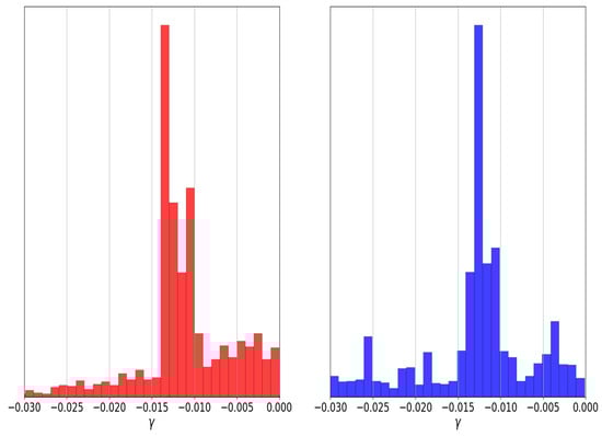
Figure 5.
Comparison between the histograms of nested sampling (red) and individuals through generations of the genetic algorithm (blue) for parameter of graduated dark energy model.
To conclude this section, it is worth noting that there are other multimodal cosmological models, mainly involving neutrinos and spatial curvature, documented in the literature [114,115,116,117,118], and it is worth exploring in future works where these techniques could prove valuable for conducting efficient and rapid assessments.
4.3. Derived Functions
As an additional application, taking advantage of the genetic algorithms’ nature, we can use the saved individuals along generations to maximize the likelihood function and calculate the derived functions to analyze their phenomenological behavior. This technique is usually used with the samples of the posterior probability with Bayesian inference algorithms, mapping the sampling of an estimated parameter to another derived one. For example, the library fgivenx [119] allows for this mapping. In the case of the individuals of likelihood optimization using genetic algorithms, the statistical meaning of the plots is not directly related to the posterior probability function; however, it can provide an idea of the behavior of the derived functions given the estimated parameters.
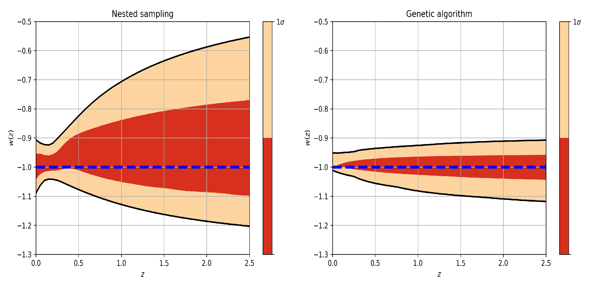
In Figure 6, we compare the equation of state reconstructed from the outputs of Section 4.1 for the CPL model, and we use the samples for the and from the nested sampling and the values of these same parameters from the history of the individuals of the genetic algorithm population. We can notice that the behavior of the equation of state, analyzing the darkest regions, is similar in both cases, and it suggests that for a quick test, we can use this technique with genetic algorithms. Regarding the confidence regions, because we are only optimizing the likelihood function with the genetic algorithms, we cannot have a formal way to estimate them correctly.

Figure 6.
Equation of state for CPL model plotted with fgivenx from (left) nested sampling and (right) genetic algorithms. ’The darker zones represent ’ and the lighter . The dotted blue line represents the value of the Equation of State to CDM.
5. Conclusions
In this study, we have leveraged genetic algorithms as an effective tool to estimate the free parameters of four cosmological models. Individuals generated in each genetic algorithm population have demonstrated the ability to achieve faster parameter estimates than those obtained using MCMC methods, thus reducing the number of likelihood function evaluations required. In addition, these genetic algorithms allow for a rapid computation of derived parameters, which adds flexibility and efficiency to the estimation process.
However, it is important to note that genetic algorithms differ from Bayesian approaches in their sampling process. While MCMC methods fully sample the posterior probability function, genetic algorithms focus on maximizing the likelihood function. This distinction implies that genetic algorithms cannot directly provide confidence regions with the same statistical significance as Bayesian inference procedures. However, they offer significant advantages, such as a faster speed and better results than other optimization methods, such as the L-BFGS algorithm.
Additionally, we have explored the usefulness of sharing and niche techniques in genetic algorithms, ensuring practical parameter space exploration, even in local or global optima. These features may be especially valuable in cosmology as a prior analysis to maximize the likelihood function before undertaking more computationally expensive Bayesian parameter estimation.
Throughout this paper, we can understand why genetic algorithms have been a very promising field of research over the last decades. Their flexibility allows for their application in diverse tasks, such as optimization, combinatorics, statistics, and even to speed up computational algorithms. The potential future applications of genetic algorithms in cosmological research are vast. With the presented study, we show the prospect of using them as a complement within cosmological data analysis. This is in agreement and complementary with the existing research that also focuses on the statistical applications of evolutionary computation [39,120]. In our case, we have not proposed a novel method or algorithm; however, we have analyzed how to use GAs so that they can complement a traditional analysis of cosmological data and be an alternative to optimize the likelihood function. We are convinced that genetic algorithms are a great technique with diverse cosmological and statistical applications. For example, in a parallel work, we have explored their usefulness to improve cosmological neural reconstructions [31] and to reduce the computational time of Bayesian inference routines. Therefore, we are confident that genetic algorithms are an excellent complementary element to the cosmological data analysis toolkit.
Author Contributions
All authors have contributed equally to all stages of the research: conceptualisation, methodology, formal analysis, and original writing draft. All authors have read and agreed to the published version of the manuscript.
Funding
This research was funded by FOSEC SEP-CONACYT Investigación Básica A1-S-21925, PRONACES-CONACYT/304001/2020, UNAM-DGAPA-PAPIIT IN117723, SIP20230505-IPN, FORDECYT-PRONACES-CONACYT CF-MG-2558591 and COFAA-IPN, and EDI-IPN grants.
Data Availability Statement
The datasets utilised comprise 31 cosmic chronometers [84,85,86,87,88,89,90,91], Baryon Acoustic Oscillation measurements (BAO) [92,93,94,95,96,97], 1048 Type Ia supernovae (SNeIa) sourced from the Pantheon compilation [98], and binned data from the Joint Light Analysis SNeIa compilation [99].
Conflicts of Interest
The authors declare no conflicts of interest.
Notes
| 1 | Let us consider a binary representation of a genetic algorithm where each individual is a sequence of binary values representing a potential solution. Suppose an individual’s chromosome (binary sequence) is 101010. A mutation operation might involve flipping one of the bits, resulting in a new chromosome, like 111010 or 100010. A mutation probability determines the choice of which bit to flip. If the mutation probability is low, only a few bits are expected to change, maintaining some of the original information. This process introduces diversity in the population, allowing the algorithm to explore different regions of the search space and preventing premature convergence to suboptimal solutions. In a genetic algorithm, a bit denotes the smallest unit of information representing a decision within a solution. Unlike a bit in memory, it symbolizes binary choices in a solution space rather than directly storing data. |
| 2 | https://igomezv.github.io/SimpleMC (accessed on 18 December 2023). |
References
- Srinivas, M.; Patnaik, L.M. Genetic algorithms: A survey. Computer 1994, 27, 17–26. [Google Scholar] [CrossRef]
- Tomassini, M. A survey of genetic algorithms. In Annual Reviews of Computational Physics III; World Scientific: Singapore, 1995; pp. 87–118. [Google Scholar]
- Mitchell, M. Genetic algorithms: An overview. Complex 1995, 1, 31–39. [Google Scholar] [CrossRef]
- Kumar, M.; Husain, M.; Upreti, N.; Gupta, D. Genetic Algorithm: Review and Application; SSRN: New York, NY, USA, 2010. [Google Scholar]
- Katoch, S.; Chauhan, S.S.; Kumar, V. A review on genetic algorithm: Past, present, and future. Multimed. Tools Appl. 2021, 80, 8091–8126. [Google Scholar] [CrossRef]
- Dumitrescu, D.; Lazzerini, B.; Jain, L.C.; Dumitrescu, A. Evolutionary Computation; CRC Press: Boca Raton, FL, USA, 2000. [Google Scholar]
- Yang, X.S. Nature-Inspired Metaheuristic Algorithms; Luniver Press: Bristol, UK, 2010. [Google Scholar]
- Sadeeq, H.T.; Abdulazeez, A.M. Metaheuristics: A Review of Algorithms. Int. J. Online Biomed. Eng. 2023, 19, 142–164. [Google Scholar] [CrossRef]
- Kennedy, J.; Eberhart, R. Particle swarm optimization. In Proceedings of the ICNN’95-International Conference on Neural Networks, Perth, Australia, 27 November–1 December 1995; IEEE: Piscataway, NJ, USA, 1995; Volume 4, pp. 1942–1948. [Google Scholar]
- Sadeeq, H.T.; Abdulazeez, A.M. Giant trevally optimizer (GTO): A novel metaheuristic algorithm for global optimization and challenging engineering problems. IEEE Access 2022, 10, 121615–121640. [Google Scholar] [CrossRef]
- Sadeeq, H.T.; Abdulazeez, A.M. Car side impact design optimization problem using giant trevally optimizer. Structures 2023, 55, 39–45. [Google Scholar] [CrossRef]
- Hashish, M.S.; Hasanien, H.M.; Ullah, Z.; Alkuhayli, A.; Badr, A.O. Giant Trevally Optimization Approach for Probabilistic Optimal Power Flow of Power Systems Including Renewable Energy Systems Uncertainty. Sustainability 2023, 15, 13283. [Google Scholar] [CrossRef]
- Wang, L.; Cao, Q.; Zhang, Z.; Mirjalili, S.; Zhao, W. Artificial rabbits optimization: A new bio-inspired meta-heuristic algorithm for solving engineering optimization problems. Eng. Appl. Artif. Intell. 2022, 114, 105082. [Google Scholar] [CrossRef]
- Alsaiari, A.O.; Moustafa, E.B.; Alhumade, H.; Abulkhair, H.; Elsheikh, A. A coupled artificial neural network with artificial rabbits optimizer for predicting water productivity of different designs of solar stills. Adv. Eng. Softw. 2023, 175, 103315. [Google Scholar] [CrossRef]
- Holland, J.H. Adaptation in Natural and Artificial Systems: An Introductory Analysis with Applications to Biology, Control, and Artificial Intelligence; MIT Press: Cambridge, MA, USA, 1992. [Google Scholar]
- Holland, J.H. Genetic algorithms and the optimal allocation of trials. SIAM J. Comput. 1973, 2, 88–105. [Google Scholar] [CrossRef]
- Langdon, W.B. Genetic Programming and Data Structures: Genetic Programming + Data Structures = Automatic Programming! Kluwer Academic Publishers: Boston, MA, USA, 1998. [Google Scholar]
- Beyer, H.G.; Schwefel, H.P. Evolution strategies—A comprehensive introduction. Nat. Comput. 2002, 1, 3–52. [Google Scholar] [CrossRef]
- Rudolph, G. Convergence analysis of canonical genetic algorithms. IEEE Trans. Neural Netw. 1994, 5, 96–101. [Google Scholar] [CrossRef]
- García, J.; Acosta, C.; Mesa, M. Genetic algorithms for mathematical optimization. J. Phys. Conf. Ser. 2020, 1448, 012020. [Google Scholar] [CrossRef]
- Anastasio, M.A.; Yoshida, H.; Nagel, R.; Nishikawa, R.M.; Doi, K. A genetic algorithm-based method for optimizing the performance of a computer-aided diagnosis scheme for detection of clustered microcalcifications in mammograms. Med. Phys. 1998, 25, 1613–1620. [Google Scholar] [CrossRef]
- Bevilacqua, A.; Campanini, R.; Lanconelli, N. A distributed genetic algorithm for parameters optimization to detect microcalcifications in digital mammograms. In Proceedings of the Workshops on Applications of Evolutionary Computation, Como, Italy, 18–20 April 2001; Springer: Berlin/Heidelberg, Germany, 2001; pp. 278–287. [Google Scholar]
- Ghaheri, A.; Shoar, S.; Naderan, M.; Hoseini, S.S. The applications of genetic algorithms in medicine. Oman Med. J. 2015, 30, 406. [Google Scholar] [CrossRef]
- Zelenkov, Y.; Reshettsov, I. Analysis of the COVID-19 pandemic using a compartmental model with time-varying parameters fitted by a genetic algorithm. Expert Syst. Appl. 2023, 224, 120034. [Google Scholar] [CrossRef]
- Esquivel, R.M.; Gómez-Vargas, I.; Montalvo, T.R.; Vázquez, J.A.; García-Salcedo, R. The inverse problem of a dynamical system solved with genetic algorithms. J. Phys. Conf. Ser. 2021, 1723, 012021. [Google Scholar] [CrossRef]
- Simpson, A.R.; Priest, S.D. The application of genetic algorithms to optimisation problems in geotechnics. Comput. Geotech. 1993, 15, 1–19. [Google Scholar] [CrossRef]
- Drachal, K.; Pawłowski, M. A review of the applications of genetic algorithms to forecasting prices of commodities. Economies 2021, 9, 6. [Google Scholar] [CrossRef]
- Victorino, I.R.d.S.; Maciel Filho, R. Application of Genetic Algorithms To the Optimization of an Industrial Reactor. IFAC Proc. Vol. 2006, 39, 857–862. [Google Scholar] [CrossRef]
- Kuri-Morales, A. Closed determination of the number of neurons in the hidden layer of a multi-layered perceptron network. Soft Comput. 2017, 21, 597–609. [Google Scholar] [CrossRef]
- Whitley, D.; Starkweather, T.; Bogart, C. Genetic algorithms and neural networks: Optimizing connections and connectivity. Parallel Comput. 1990, 14, 347–361. [Google Scholar] [CrossRef]
- Gómez-Vargas, I.; Andrade, J.B.; Vázquez, J.A. Neural networks optimized by genetic algorithms in cosmology. Phys. Rev. D 2023, 107, 043509. [Google Scholar] [CrossRef]
- Abel, S.; Constantin, A.; Harvey, T.R.; Lukas, A. Evolving Heterotic Gauge Backgrounds: Genetic Algorithms versus Reinforcement Learning. Fortschritte Der Phys. 2022, 70, 2200034. [Google Scholar] [CrossRef]
- Bourilkov, D. Machine and deep learning applications in particle physics. Int. J. Mod. Phys. A 2019, 34, 1930019. [Google Scholar] [CrossRef]
- Akrami, Y.; Scott, P.; Edsjö, J.; Conrad, J.; Bergström, L. A profile likelihood analysis of the constrained MSSM with genetic algorithms. J. High Energy Phys. 2010, 2010, 57. [Google Scholar] [CrossRef]
- Charbonneau, P. Genetic algorithms in astronomy and astrophysics. Astrophys. J. Suppl. 1995, 101, 309. [Google Scholar] [CrossRef]
- Fridman, P. Radio astronomy image enhancement in the presence of phase errors using genetic algorithms. In Proceedings of the 2001 International Conference on Image Processing (Cat. No. 01CH37205), Thessaloniki, Greece, 7–10 October 2001; IEEE: Piscataway, NJ, USA, 2001; Volume 3, pp. 612–615. [Google Scholar]
- Rajpaul, V. Genetic algorithms in astronomy and astrophysics. arXiv 2012, arXiv:1202.1643. [Google Scholar]
- Holl, B.; Sozzetti, A.; Sahlmann, J.; Giacobbe, P.; Ségransan, D.; Unger, N.; Delisle, J.B.; Barbato, D.; Lattanzi, M.; Morbidelli, R.; et al. Gaia Data Release 3-Astrometric orbit determination with Markov chain Monte Carlo and genetic algorithms: Systems with stellar, sub-stellar, and planetary mass companions. Astron. Astrophys. 2023, 674, A10. [Google Scholar] [CrossRef]
- Axiak, M.; Kitching, T.; van Hemert, J. Evolution Strategies for Cosmology: A Comparison of Nested Sampling Methods. arXiv 2011, arXiv:1101.0717. [Google Scholar]
- Luo, X.L.; Feng, J.; Zhang, H.H. A genetic algorithm for astroparticle physics studies. Comput. Phys. Commun. 2020, 250, 106818. [Google Scholar] [CrossRef]
- Gómez-Vargas, I.; Medel-Esquivel, R.; García-Salcedo, R.; Vázquez, J.A. Neural network reconstructions for the Hubble parameter, growth rate and distance modulus. Eur. Phys. J. C 2023, 83, 304. [Google Scholar] [CrossRef]
- Kamerkar, A.; Nesseris, S.; Pinol, L. Machine learning cosmic inflation. Phys. Rev. D 2023, 108, 043509. [Google Scholar] [CrossRef]
- Chacón, J.; Gómez-Vargas, I.; Méndez, R.M.; Vázquez, J.A. Analysis of dark matter halo structure formation in N-body simulations with machine learning. Phys. Rev. D 2023, 107, 123515. [Google Scholar] [CrossRef]
- de Dios Rojas Olvera, J.; Gómez-Vargas, I.; Vázquez, J.A. Observational cosmology with artificial neural networks. Universe 2022, 8, 120. [Google Scholar] [CrossRef]
- Arjona, R.; Nesseris, S. What can Machine Learning tell us about the background expansion of the Universe? Phys. Rev. D 2020, 101, 123525. [Google Scholar] [CrossRef]
- Nesseris, S.; Garcia-Bellido, J. A new perspective on Dark Energy modeling via Genetic Algorithms. J. Cosmol. Astropart. Phys. 2012, 2012, 033. [Google Scholar] [CrossRef]
- Wang, K.; Guo, P.; Yu, F.; Duan, L.; Wang, Y.; Du, H. Computational intelligence in astronomy: A survey. Int. J. Comput. Intell. Syst. 2018, 11, 575. [Google Scholar] [CrossRef]
- Bogdanos, C.; Nesseris, S. Genetic algorithms and supernovae type Ia analysis. J. Cosmol. Astropart. Phys. 2009, 2009, 6. [Google Scholar] [CrossRef]
- Nesseris, S.; Shafieloo, A. A model-independent null test on the cosmological constant. Mon. Not. R. Astron. Soc. 2010, 408, 1879–1885. [Google Scholar] [CrossRef]
- Alestas, G.; Kazantzidis, L.; Nesseris, S. Machine learning constraints on deviations from general relativity from the large scale structure of the Universe. Phys. Rev. D 2022, 106, 103519. [Google Scholar] [CrossRef]
- Pellejero-Ibáñez, M.; Angulo, R.E.; Aricó, G.; Zennaro, M.; Contreras, S.; Stücker, J. Cosmological parameter estimation via iterative emulation of likelihoods. Mon. Not. R. Astron. Soc. 2020, 499, 5257–5268. [Google Scholar] [CrossRef]
- Wraith, D.; Wraith, D.; Kilbinger, M.; Benabed, K.; Capp’e, O.; Cardoso, J.F.; Cardoso, J.F.; Fort, G.; Prunet, S.; Robert, C.P. Estimation of cosmological parameters using adaptive importance sampling. Phys. Rev. D 2009, 80, 023507. [Google Scholar] [CrossRef]
- Graff, P.; Feroz, F.; Hobson, M.P.; Lasenby, A. BAMBI: Blind accelerated multimodal Bayesian inference. Mon. Not. R. Astron. Soc. 2012, 421, 169–180. [Google Scholar] [CrossRef]
- Nygaard, A.; Holm, E.B.; Hannestad, S.; Tram, T. CONNECT: A neural network based framework for emulating cosmological observables and cosmological parameter inference. J. Cosmol. Astropart. Phys. 2023, 2023, 025. [Google Scholar] [CrossRef]
- Gómez-Vargas, I.; Esquivel, R.M.; García-Salcedo, R.; Vázquez, J.A. Neural network within a bayesian inference framework. J. Phys. Conf. Ser. 2021, 1723, 012022. [Google Scholar] [CrossRef]
- Alsing, J.; Charnock, T.; Feeney, S.; Wandelt, B. Fast likelihood-free cosmology with neural density estimators and active learning. Mon. Not. R. Astron. Soc. 2019, 488, 4440–4458. [Google Scholar] [CrossRef]
- Leclercq, F. Bayesian optimization for likelihood-free cosmological inference. Phys. Rev. D 2018, 98, 063511. [Google Scholar] [CrossRef]
- Bagavathi, C.; Saraniya, O. Evolutionary Mapping Techniques for Systolic Computing System. In Deep Learning and Parallel Computing Environment for Bioengineering Systems; Elsevier: Amsterdam, The Netherlands, 2019; pp. 207–223. [Google Scholar]
- Passino, K.M. Biomimicry of bacterial foraging for distributed optimization and control. IEEE Control Syst. Mag. 2002, 22, 52–67. [Google Scholar]
- Mirjalili, S.; Mirjalili, S.M.; Lewis, A. Grey wolf optimizer. Adv. Eng. Softw. 2014, 69, 46–61. [Google Scholar] [CrossRef]
- Faris, H.; Aljarah, I.; Al-Betar, M.A.; Mirjalili, S. Grey wolf optimizer: A review of recent variants and applications. Neural Comput. Appl. 2018, 30, 413–435. [Google Scholar] [CrossRef]
- Simon, D. Biogeography-based optimization. IEEE Trans. Evol. Comput. 2008, 12, 702–713. [Google Scholar] [CrossRef]
- Mitchell, M. An Introduction to Genetic Algorithms; MIT Press: Cambridge, MA, USA, 1998. [Google Scholar]
- Waddington, C.H. An Introduction to Modern Genetics; Routledge: London, UK, 2016. [Google Scholar]
- Kumar, A. Encoding schemes in genetic algorithm. Int. J. Adv. Res. Eng. 2013, 2, 1–7. [Google Scholar]
- Beasley, D.; Bull, D.R.; Martin, R.R. An overview of genetic algorithms: Part 1, fundamentals. Univ. Comput. 1993, 15, 56–69. [Google Scholar]
- Mirjalili, S.; Mirjalili, S. Genetic algorithm. Evolutionary Algorithms and Neural Networks: Theory and Applications; Springer: Cham, Switzerland, 2019; pp. 43–55. [Google Scholar]
- Sivanandam, S.; Deepa, S.; Sivanandam, S.; Deepa, S. Genetic Algorithms; Springer: Berlin/Heidelberg, Germany, 2008. [Google Scholar]
- Goldberg, D.E.; Deb, K. A comparative analysis of selection schemes used in genetic algorithms. In Foundations of Genetic Algorithms; Elsevier: Amsterdam, The Netherlands, 1991; Volume 1, pp. 69–93. [Google Scholar]
- Miller, B.L.; Goldberg, D.E. Genetic algorithms, tournament selection, and the effects of noise. Complex Syst. 1995, 9, 193–212. [Google Scholar]
- Lee, C.Y. Entropy-Boltzmann selection in the genetic algorithms. IEEE Trans. Syst. Man Cybern. Part B (Cybern.) 2003, 33, 138–149. [Google Scholar]
- Marsili Libelli, S.; Alba, P. Adaptive mutation in genetic algorithms. Soft Comput. 2000, 4, 76–80. [Google Scholar] [CrossRef]
- Fortin, F.A.; De Rainville, F.M. Distributed Evolutionary Algorithms. Available online: https://github.com/deap (accessed on 18 December 2023).
- Staats, K. Karoo_gp. Available online: http://kstaats.github.io/karoo_gp/ (accessed on 18 December 2023).
- Sipper, M. Tiny Genetic Programming. Available online: https://github.com/moshesipper/tiny_gp (accessed on 18 December 2023).
- Bonson, J.P.C. Symbiotic Bid-Based GP. Available online: https://github.com/jpbonson/SBBFramework (accessed on 18 December 2023).
- Wirsansky, E. Hands-On Genetic Algorithms with Python: Applying Genetic Algorithms to Solve Real-World Deep Learning and Artificial Intelligence Problems; Packt Publishing: Birmingham, UK, 2020. [Google Scholar]
- Eiben, A.E.; Rudolph, G. Theory of evolutionary algorithms: A bird’s eye view. Theor. Comput. Sci. 1999, 229, 3–9. [Google Scholar] [CrossRef]
- Oliveto, P.S.; Witt, C. On the runtime analysis of the simple genetic algorithm. Theor. Comput. Sci. 2014, 545, 2–19. [Google Scholar] [CrossRef]
- Šílenỳ, J. Earthquake source parameters and their confidence regions by a genetic algorithm with a ‘memory’. Geophys. J. Int. 1998, 134, 228–242. [Google Scholar] [CrossRef]
- Esquivel, R.M.; Gómez-Vargas, I.; Vázquez, J.A.; Salcedo, R.G. An introduction to Markov Chain Monte Carlo. Boletín EstadíStica Investig. Oper. 2021, 1, 47–74. [Google Scholar]
- Hogg, D.W.; Foreman-Mackey, D. Data analysis recipes: Using markov chain monte carlo. Astrophys. J. Suppl. Ser. 2018, 236, 11. [Google Scholar] [CrossRef]
- Akarsu, Ö.; Barrow, J.D.; Escamilla, L.A.; Vazquez, J.A. Graduated dark energy: Observational hints of a spontaneous sign switch in the cosmological constant. Phys. Rev. D 2020, 101, 063528. [Google Scholar] [CrossRef]
- Jimenez, R.; Verde, L.; Treu, T.; Stern, D. Constraints on the equation of state of dark energy and the Hubble constant from stellar ages and the cosmic microwave background. Astrophys. J. 2003, 593, 622. [Google Scholar] [CrossRef]
- Simon, J.; Verde, L.; Jimenez, R. Constraints on the redshift dependence of the dark energy potential. Phys. Rev. D 2005, 71, 123001. [Google Scholar] [CrossRef]
- Stern, D.; Jimenez, R.; Verde, L.; Kamionkowski, M.; Stanford, S.A. Cosmic chronometers: Constraining the equation of state of dark energy. I: H(z) measurements. J. Cosmol. Astropart. Phys. 2010, 2010, 008. [Google Scholar] [CrossRef]
- Moresco, M.; Verde, L.; Pozzetti, L.; Jimenez, R.; Cimatti, A. New constraints on cosmological parameters and neutrino properties using the expansion rate of the Universe to z ∼ 1.75. J. Cosmol. Astropart. Phys. 2012, 2012, 053. [Google Scholar] [CrossRef]
- Zhang, C.; Zhang, H.; Yuan, S.; Liu, S.; Zhang, T.J.; Sun, Y.C. Four new observational H(z) data from luminous red galaxies in the Sloan Digital Sky Survey data release seven. Res. Astron. Astrophys. 2014, 14, 1221. [Google Scholar] [CrossRef]
- Moresco, M. Raising the bar: New constraints on the Hubble parameter with cosmic chronometers at z ∼ 2. Mon. Not. R. Astron. Soc. Lett. 2015, 450, L16–L20. [Google Scholar] [CrossRef]
- Moresco, M.; Pozzetti, L.; Cimatti, A.; Jimenez, R.; Maraston, C.; Verde, L.; Thomas, D.; Citro, A.; Tojeiro, R.; Wilkinson, D. A 6% measurement of the Hubble parameter at z ∼ 0.45: Direct evidence of the epoch of cosmic re-acceleration. J. Cosmol. Astropart. Phys. 2016, 2016, 014. [Google Scholar] [CrossRef]
- Ratsimbazafy, A.; Loubser, S.; Crawford, S.; Cress, C.; Bassett, B.; Nichol, R.; Väisänen, P. Age-dating luminous red galaxies observed with the Southern African Large Telescope. Mon. Not. R. Astron. Soc. 2017, 467, 3239–3254. [Google Scholar] [CrossRef]
- Alam, S.; Ata, M.; Bailey, S.; Beutler, F.; Bizyaev, D.; Blazek, J.A.; Bolton, A.S.; Brownstein, J.R.; Burden, A.; Chuang, C.H.; et al. The clustering of galaxies in the completed SDSS-III Baryon Oscillation Spectroscopic Survey: Cosmological analysis of the DR12 galaxy sample. Mon. Not. R. Astron. Soc. 2017, 470, 2617–2652. [Google Scholar] [CrossRef]
- Ata, M.; Baumgarten, F.; Bautista, J.; Beutler, F.; Bizyaev, D.; Blanton, M.R.; Blazek, J.A.; Bolton, A.S.; Brinkmann, J.; Brownstein, J.R.; et al. The clustering of the SDSS-IV extended Baryon Oscillation Spectroscopic Survey DR14 quasar sample: First measurement of baryon acoustic oscillations between redshift 0.8 and 2.2. Mon. Not. R. Astron. Soc. 2018, 473, 4773–4794. [Google Scholar] [CrossRef]
- Blomqvist, M.; Des Bourboux, H.D.M.; de Sainte Agathe, V.; Rich, J.; Balland, C.; Bautista, J.E.; Dawson, K.; Font-Ribera, A.; Guy, J.; Le Goff, J.M.; et al. Baryon acoustic oscillations from the cross-correlation of Lyα absorption and quasars in eBOSS DR14. Astron. Astrophys. 2019, 629, A86. [Google Scholar] [CrossRef]
- de Sainte Agathe, V.; Balland, C.; Des Bourboux, H.D.M.; Blomqvist, M.; Guy, J.; Rich, J.; Font-Ribera, A.; Pieri, M.M.; Bautista, J.E.; Dawson, K.; et al. Baryon acoustic oscillations at z = 2.34 from the correlations of Lyα absorption in eBOSS DR14. Astron. Astrophys. 2019, 629, A85. [Google Scholar] [CrossRef]
- Beutler, F.; Blake, C.; Colless, M.; Jones, D.H.; Staveley-Smith, L.; Campbell, L.; Parker, Q.; Saunders, W.; Watson, F. The 6dF Galaxy Survey: Baryon acoustic oscillations and the local Hubble constant. Mon. Not. R. Astron. Soc. 2011, 416, 3017–3032. [Google Scholar] [CrossRef]
- Ross, A.J.; Samushia, L.; Howlett, C.; Percival, W.J.; Burden, A.; Manera, M. The clustering of the SDSS DR7 main Galaxy sample–I. A 4 per cent distance measure at z = 0.15. Mon. Not. R. Astron. Soc. 2015, 449, 835–847. [Google Scholar] [CrossRef]
- Scolnic, D.M.; Jones, D.; Rest, A.; Pan, Y.; Chornock, R.; Foley, R.; Huber, M.; Kessler, R.; Narayan, G.; Riess, A.; et al. The complete light-curve sample of spectroscopically confirmed SNe Ia from Pan-STARRS1 and cosmological constraints from the combined pantheon sample. Astrophys. J. 2018, 859, 101. [Google Scholar] [CrossRef]
- Betoule, M.; Kessler, R.; Guy, J.; Mosher, J.; Hardin, D.; Biswas, R.; Astier, P.; El-Hage, P.; Konig, M.; Kuhlmann, S.; et al. Improved cosmological constraints from a joint analysis of the SDSS-II and SNLS supernova samples. Astron. Astrophys. 2014, 568, A22. [Google Scholar] [CrossRef]
- Vazquez, J.; Gomez-Vargas, I.; Slosar, A. Updated Version of a Simple MCMC Code for Cosmological Parameter Estimation Where Only Expansion History Matters. 2023. Available online: https://github.com/ja-vazquez/SimpleMC (accessed on 18 December 2023).
- Skilling, J. Nested sampling. AIP Conf. Proc. 2004, 735, 395–405. [Google Scholar]
- Padilla, L.E.; Tellez, L.O.; Escamilla, L.A.; Vazquez, J.A. Cosmological parameter inference with Bayesian statistics. Universe 2021, 7, 213. [Google Scholar] [CrossRef]
- Sivia, D.; Skilling, J. Data Analysis: A Bayesian Tutorial; OUP, Oxford University Press: Oxford, UK, 2006. [Google Scholar]
- Zhu, C.; Byrd, R.H.; Lu, P.; Nocedal, J. Algorithm 778: L-BFGS-B: Fortran subroutines for large-scale bound-constrained optimization. ACM Trans. Math. Softw. (TOMS) 1997, 23, 550–560. [Google Scholar] [CrossRef]
- Liddle, A. An Introduction to Modern Cosmology; John Wiley & Sons: Hoboken, NJ, USA, 2015. [Google Scholar]
- Linden, S.; Virey, J.M. Test of the Chevallier-Polarski-Linder parametrization for rapid dark energy equation of state transitions. Phys. Rev. D 2008, 78, 023526. [Google Scholar] [CrossRef]
- Vazquez, J.A.; Hee, S.; Hobson, M.; Lasenby, A.; Ibison, M.; Bridges, M. Observational constraints on conformal time symmetry, missing matter and double dark energy. J. Cosmol. Astropart. Phys. 2018, 2018, 062. [Google Scholar] [CrossRef]
- Zhai, Z.; Blanton, M.; Slosar, A.; Tinker, J. An evaluation of cosmological models from the expansion and growth of structure measurements. Astrophys. J. 2017, 850, 183. [Google Scholar] [CrossRef]
- Feroz, F.; Hobson, M.; Bridges, M. MultiNest: An efficient and robust Bayesian inference tool for cosmology and particle physics. Mon. Not. R. Astron. Soc. 2009, 398, 1601–1614. [Google Scholar] [CrossRef]
- Acquaviva, G.; Akarsu, Ö.; Katırcı, N.; Vazquez, J.A. Simple-graduated dark energy and spatial curvature. Phys. Rev. D 2021, 104, 023505. [Google Scholar] [CrossRef]
- Akarsu, Ö.; Kumar, S.; Özülker, E.; Vazquez, J.A. Relaxing cosmological tensions with a sign switching cosmological constant. Phys. Rev. D 2021, 104, 123512. [Google Scholar] [CrossRef]
- Akarsu, O.; Di Valentino, E.; Kumar, S.; Nunes, R.C.; Vazquez, J.A.; Yadav, A. LambdasCDM model: A promising scenario for alleviation of cosmological tensions. arXiv 2023, arXiv:2307.10899. [Google Scholar]
- Akarsu, Ö.; Kumar, S.; Özülker, E.; Vazquez, J.A.; Yadav, A. Relaxing cosmological tensions with a sign switching cosmological constant: Improved results with Planck, BAO, and Pantheon data. Phys. Rev. D 2023, 108, 023513. [Google Scholar] [CrossRef]
- Kreisch, C.D.; Park, M.; Calabrese, E.; Cyr-Racine, F.Y.; An, R.; Bond, J.R.; Dore, O.; Dunkley, J.; Gallardo, P.; Gluscevic, V.; et al. The Atacama Cosmology Telescope: The Persistence of Neutrino Self-Interaction in Cosmological Measurements. arXiv 2022, arXiv:2207.03164. [Google Scholar]
- Camarena, D.; Cyr-Racine, F.Y.; Houghteling, J. The two-mode puzzle: Confronting self-interacting neutrinos with the full shape of the galaxy power spectrum. arXiv 2023, arXiv:2309.03941. [Google Scholar]
- Cedeno, F.X.L.; Nucamendi, U. Revisiting cosmological diffusion models in Unimodular Gravity and the H0 tension. Phys. Dark Universe 2021, 32, 100807. [Google Scholar] [CrossRef]
- Park, M.; Kreisch, C.D.; Dunkley, J.; Hadzhiyska, B.; Cyr-Racine, F.Y. Λ CDM or self-interacting neutrinos: How CMB data can tell the two models apart. Phys. Rev. D 2019, 100, 063524. [Google Scholar] [CrossRef]
- de Cruz Pérez, J.; Park, C.G.; Ratra, B. Current data are consistent with flat spatial hypersurfaces in the Λ CDM cosmological model but favor more lensing than the model predicts. Phys. Rev. D 2023, 107, 063522. [Google Scholar] [CrossRef]
- Handley, W. fgivenx: A Python package for functional posterior plotting. arXiv 2019, arXiv:1908.01711. [Google Scholar] [CrossRef]
- Surendran, S.P.; Thomas, R.; Joy, M. Evolutionary optimization of cosmological parameters using metropolis acceptance criterion. arXiv 2022, arXiv:2205.01752. [Google Scholar]


Disclaimer/Publisher’s Note: The statements, opinions and data contained in all publications are solely those of the individual author(s) and contributor(s) and not of MDPI and/or the editor(s). MDPI and/or the editor(s) disclaim responsibility for any injury to people or property resulting from any ideas, methods, instructions or products referred to in the content. |
© 2023 by the authors. Licensee MDPI, Basel, Switzerland. This article is an open access article distributed under the terms and conditions of the Creative Commons Attribution (CC BY) license (https://creativecommons.org/licenses/by/4.0/).