
Two-Stage Deep-Learning Classifier for Diagnostics of Lung Cancer Using Metabolites

 ,
,
Abstract
:1. Introduction
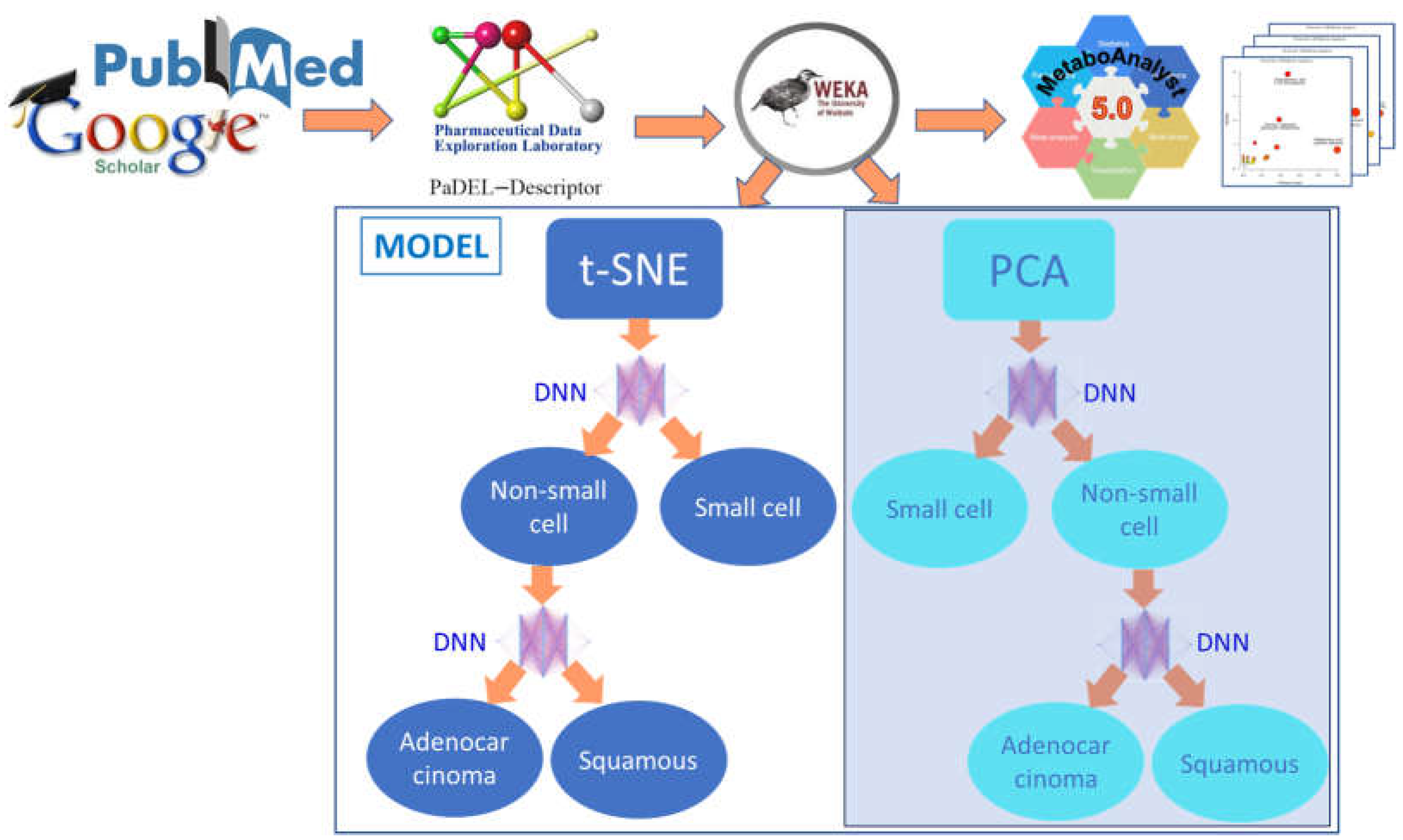
2. Methods
2.1. Datasets for Cancer Classifications
2.2. MetaboAnalyst
2.3. Raw Data and Physiochemical Descriptors
2.4. Discretization and InfoGain
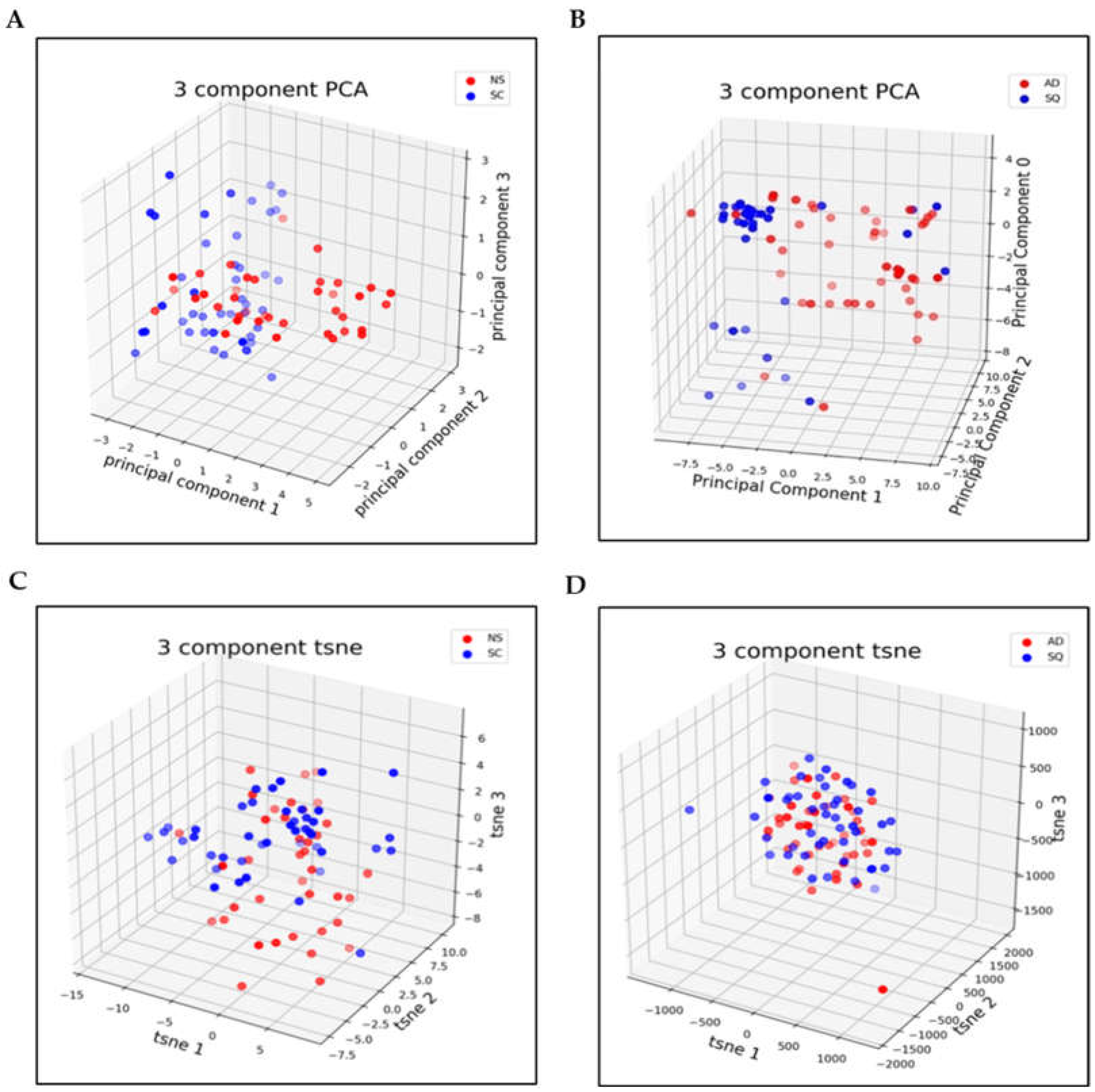
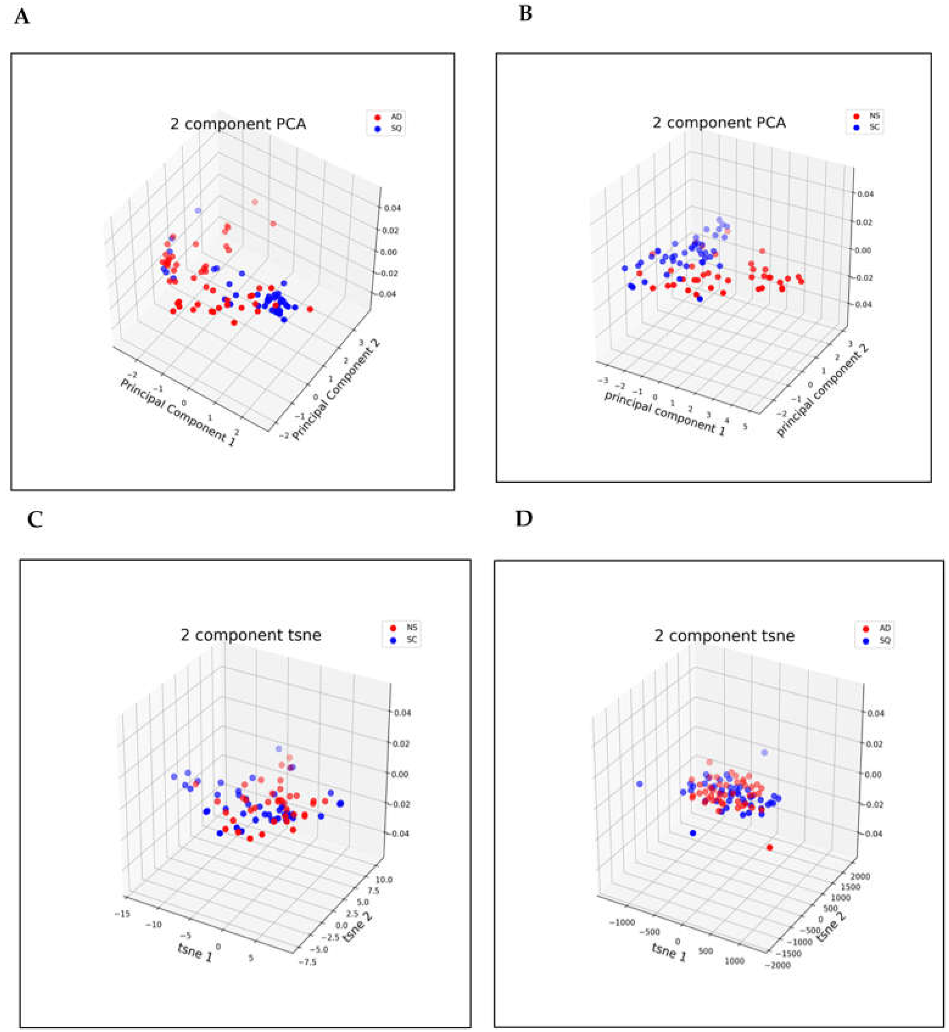
2.5. Dimensionality Reduction
2.6. Dimensionality Reduction for NS/SC
2.7. Dimensionality Reduction for AD/SQ
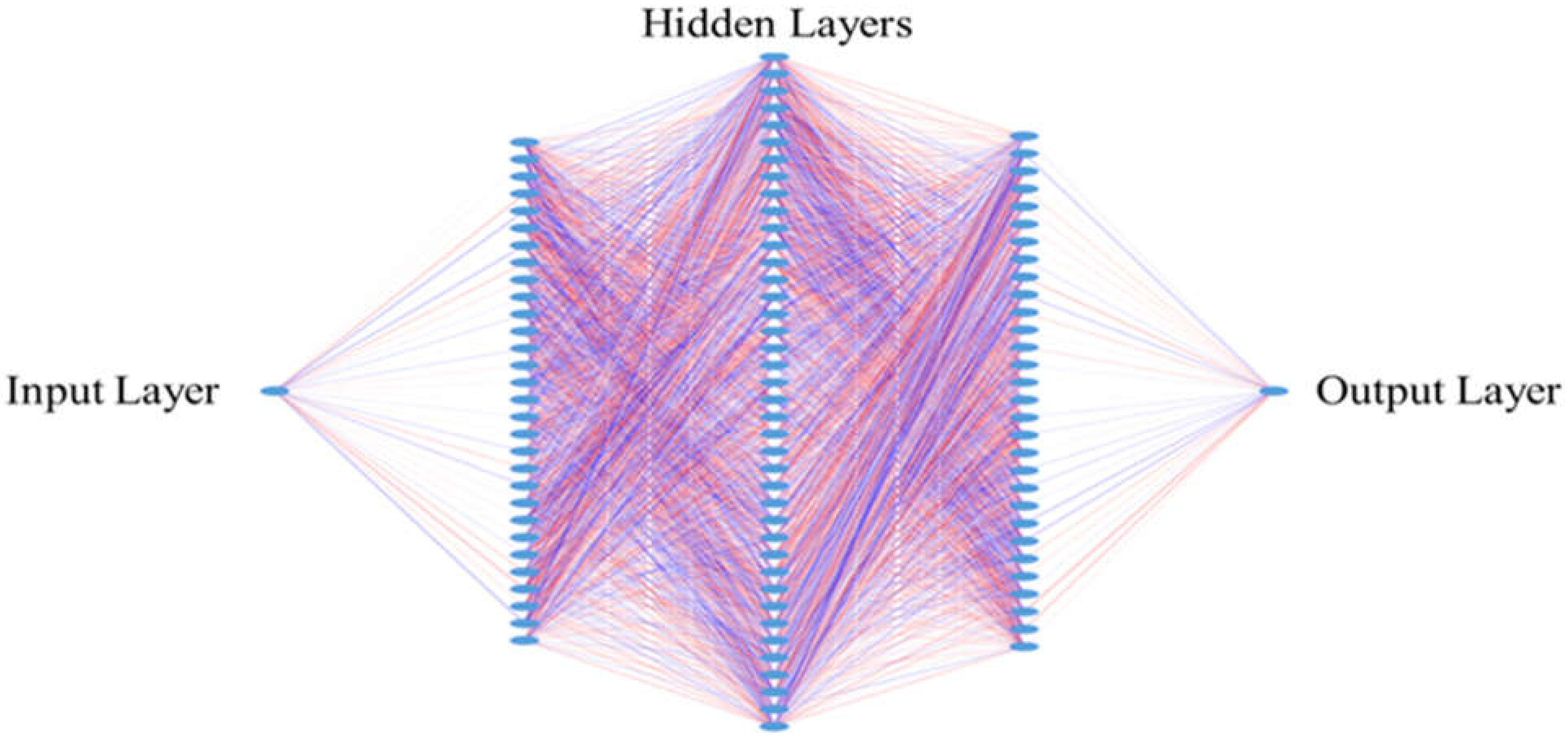
2.8. Design for the Neural Networks
2.9. Hyperparameters
3. Results
3.1. Important Pathways for Lung Cancers
3.1.1. Important Pathways for Non-Small-Cell Lung Cancers
3.1.2. Important Pathways for Adenocarcinoma Lung Cancers
3.1.3. Important Pathways for Squamous Cell Lung Cancers
3.1.4. Small-Cell Carcinoma Pathways
3.2. Dimensionality Reduction
3.3. Metrics
4. Discussion
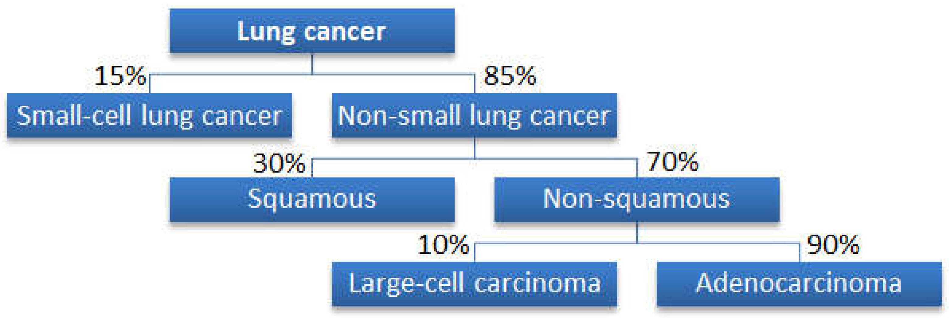
Why Is a Tree Structure Needed?
5. Future Work
6. Conclusions
Supplementary Materials
Author Contributions
Funding
Institutional Review Board Statement
Informed Consent Statement
Data Availability Statement
Conflicts of Interest
Acronyms and Abbreviations
References
- SEER. Cancer of the Lung and Bronchus—Cancer Stat Facts. Available online: https://seer.cancer.gov/statfacts/html/lungb.html (accessed on 14 May 2023).
- Petkevicius, J.; Simeliunaite, I.; Zaveckiene, J. Multivariable appearance of LAC and its subtypes on CT images. In Proceedings of the ESTI ESCR 2018 Congress, Geneva, Switzerland, 24–26 May 2018; Poster Number P-0086. Available online: https://epos.myesr.org/poster/esr/esti-escr2018/P-0086 (accessed on 10 January 2023).
- Denisenko, T.V.; Budkevich, I.N.; Zhivotovsky, B. Cell death-based treatment of lung adenocarcinoma. Cell Death Dis. 2018, 9, 117. [Google Scholar] [CrossRef]
- Bernhardt, E.B.; Jalal, S.I. Small Cell Lung Cancer. In Lung Cancer: Treatment and Research; Reckamp, K.L., Ed.; Cancer Treatment and Research; Springer: Cham, Switzerland, 2016; Volume 170, pp. 301–322. [Google Scholar] [CrossRef]
- Huang, T.; Li, J.; Zhang, C.; Hong, Q.; Jiang, D.; Ye, M.; Duan, S. Distinguishing lung adenocarcinoma from lung squamous cell carcinoma by two hypomethylated and three hypermethylated genes: A meta-analysis. PLoS ONE 2016, 11, e0149088. [Google Scholar] [CrossRef] [PubMed]
- del Ciello, A.; Franchi, P.; Contegiacomo, A.; Cicchetti, G.; Bonomo, L.; Larici, A.R. Missed lung cancer: When, where, and why? Diagn. Interv. Radiol. 2017, 23, 118–126. [Google Scholar] [CrossRef] [PubMed]
- Ratnapalan, S.; Bentur, Y.; Koren, G. Doctor, will that x-ray harm my unborn child? Can. Med. Assoc. J. 2008, 179, 1293–1296. [Google Scholar] [CrossRef]
- Mazzone, P.J.; Wang, X.-F.; Beukemann, M.; Zhang, Q.; Seeley, M.; Mohney, R.; Holt, T.; Pappan, K.L. Metabolite profiles of the serum of patients with non–small cell carcinoma. J. Thorac. Oncol. 2016, 11, 72–78. [Google Scholar] [CrossRef] [PubMed]
- Kouznetsova, V.L.; Kim, E.; Romm, E.L.; Zhu, A.; Tsigelny, I.F. Recognition of early and late stages of bladder cancer using metabolites and machine learning. Metabolomics 2019, 15, 94. [Google Scholar] [CrossRef] [PubMed]
- Kouznetsova, V.L.; Li, J.; Romm, E.; Tsigelny, I.F. Finding distinctions between oral cancer and periodontitis using saliva metabolites and machine learning. Oral Dis. 2021, 27, 484–493. [Google Scholar] [CrossRef]
- Wu, J.; Zan, X.; Gao, L.; Zhao, J.; Fan, J.; Shi, H.; Wan, Y.; Yu, E.; Li, S.; Xie, X.A. Machine learning method for identifying lung cancer based on routine blood indices: Qualitative feasibility study. JMIR Med. Inform. 2019, 7, e13476. [Google Scholar] [CrossRef]
- Fahrmann, J.F.; Kim, K.; DeFelice, B.C.; Taylor, S.L.; Gandara, D.R.; Yoneda, K.Y.; Cooke, D.T.; Fiehn, O.; Kelly, K.; Miyamoto, S. Investigation of metabolomic blood biomarkers for detection of adenocarcinoma lung cancer. Cancer Epidemiol. Biomark. Prev. 2015, 24, 1716–1723. [Google Scholar] [CrossRef]
- Chong, J.; Soufan, O.; Li, C.; Caraus, I.; Li, S.; Bourque, G.; Wishart, D.S.; Xia, J. MetaboAnalyst 4.0: Towards more transparent and integrative metabolomics analysis. Nucleic Acids Res. 2018, 46, W486–W494. [Google Scholar] [CrossRef]
- Chen, Y.; Ma, Z.; Zhong, J.; Li, L.; Min, L.; Xu, L.; Li, H.; Zhang, J.; Wu, W.; Dai, L. Simultaneous quantification of serum monounsaturated and polyunsaturated phosphatidylcholines as potential biomarkers for diagnosing non-small cell lung cancer. Sci. Rep. 2018, 8, 7137. [Google Scholar] [CrossRef]
- Wedge, D.C.; Allwood, J.W.; Dunn, W.; Vaughan, A.A.; Simpson, K.; Brown, M.; Priest, L.; Blackhall, F.H.; Whetton, A.D.; Dive, C.; et al. Is serum or plasma more appropriate for intersubject comparisons in metabolomic studies? An assessment in patients with small-cell lung cancer. Anal. Chem. 2011, 83, 6689–6697. [Google Scholar] [CrossRef] [PubMed]
- Yu, L.; Li, K.; Xu, Z.; Cui, G.; Zhang, X. Integrated omics and gene expression analysis identifies the loss of metabolite–Metabolite correlations in small cell lung cancer. OncoTargets Ther. 2018, 11, 3919–3929. [Google Scholar] [CrossRef] [PubMed]
- Liu, J.; Mazzone, P.J.; Cata, J.P.; Kurz, A.; Bauer, M.; Mascha, E.J.; Sessler, D.I. Serum free fatty acid biomarkers of lung cancer. Chest 2014, 146, 670–679. [Google Scholar] [CrossRef] [PubMed]
- Yap, C.W. PaDEL-descriptor: An open source software to calculate molecular descriptors and fingerprints. J. Comput. Chem. 2011, 32, 1466–1474. [Google Scholar] [CrossRef]
- Alam, M. Data Normalization in Machine Learning. Towards Data Science. December 2020. Available online: https://towardsdatascience.com/data-normalization-in-machine-learning-395fdec69d02 (accessed on 3 March 2023).
- Hall, M. weka.attributeSelection. Class InfoGainAttributeEval. Available online: https://weka.sourceforge.io/doc.dev/weka/attributeSelection/InfoGainAttributeEval.html (accessed on 4 March 2023).
- Lutes, J. Entropy and Information Gain in Decision Trees. Towards Data Science. November 2020. Available online: https://towardsdatascience.com/entropy-and-information-gain-in-decision-trees-c7db67a3a293 (accessed on 4 March 2023).
- Jolliffe, I. Principal component analysis. In International Encyclopedia of Statistical Science, 2011th ed.; Lovric, M., Ed.; Springer: Berlin, Germany, 2010; pp. 1094–1096. [Google Scholar] [CrossRef]
- van der Maaten, L.; Hinton, G. Visualizing non-metric similarities in multiple maps. Mach. Learn. 2012, 87, 33–55. [Google Scholar] [CrossRef]
- Tripathy, B.K.; Anveshrithaa, S.; Ghela, S. Unsupervised Learning Approaches for Dimensionality Reduction and Data Visualization, 1st ed.; CRC Press: Boca Raton, FL, USA, 2022; Chapter 13, t-Distributed stochastic neighbor embedding (t-SNE); pp. 127–135. [Google Scholar]
- Jerfel, G.; Wang, S.; Wong-Fannjiang, C.; Heller, K.A.; Ma, Y.; Jordan, M.I. Variational refinement for importance sampling using the forward Kullback-Leibler divergence. In Proceedings of the Thirty-Seventh Conference on Uncertainty in Artificial Intelligence, Online, 27–30 July 2021. JMLR Press: Cambridge, MA, USA, 2021; Volume 161, pp. 1819–1829. Available online: https://proceedings.mlr.press/v161/jerfel21a.html (accessed on 22 April 2023).
- Kingma, D.P.; Ba, J. Adam: A method for stochastic optimization. arXiv 2017, arXiv:1412.6980. [Google Scholar]
- Dhillon, K.K.; Gupta, S. Biochemistry, ketogenesis. In StatPearls [Internet]; StatPearls Publishing: Treasure Island, FL, USA, 2023. Available online: https://www.ncbi.nlm.nih.gov/books/NBK493179/ (accessed on 8 March 2023).
- Reinfeld, B.I.; Madden, M.Z.; Wolf, M.M.; Chytil, A.; Bader, J.E.; Patterson, A.R.; Sugiura, A.; Cohen, A.S.; Ali, A.; Do, B.T.; et al. Cell-programmed nutrient partitioning in the tumour microenvironment. Nature 2021, 593, 282–288. [Google Scholar] [CrossRef]
- Osman, C.; Voelker, D.R.; Langer, T. Making heads or tails of phospholipids in mitochondria. J. Cell Biol. 2011, 192, 7–16. [Google Scholar] [CrossRef]
- Dolce, V.; Capello, A.R.; Lappano, R.; Maggiolini, M. Glycerophospholipid synthesis as a novel drug target against cancer. Curr. Mol. Pharmacol. 2011, 4, 167–175. [Google Scholar] [CrossRef]
- Wu, G.; Lupton, J.R.; Turner, N.D.; Fang, Y.-Z.; Yang, S. Glutathione metabolism and its implications for health. J. Nutr. 2004, 134, 489–492. [Google Scholar] [CrossRef] [PubMed]
- Bansal, A.; Celeste Simon, M. Glutathione metabolism in cancer progression and treatment resistance. J. Cell Biol. 2018, 217, 2291–2298. [Google Scholar] [CrossRef] [PubMed]
- Leonardi, R.; Jackowski, S. Biosynthesis of pantothenic acid and coenzyme A. EcoSal Plus 2007, 2, 10-1128. [Google Scholar] [CrossRef] [PubMed]
- Brosnan, J.T.; Brosnan, M.E. The sulfur-containing amino acids: An overview. J. Nutr. 2006, 136, 1636S–1640S. [Google Scholar] [CrossRef]
- Hösli, L.; Andrès, P.F.; Hösli, E. Ionic mechanisms associated with the depolarization by glutamate and aspartate on human and rat spinal neurones in tissue culture. Pflügers Archiv. 1976, 363, 43–48. [Google Scholar] [CrossRef]
- Clancy, S.; Brown, W. Translation: DNA to mRNA to protein. Nat. Educ. 2008, 1, 101. [Google Scholar]
- Cerri, R.; Barros, R.C.; de Carvalho, A.C. Hierarchical multi-label classification using local neural networks. J. Comput. Syst. Sci. 2014, 80, 39–56. [Google Scholar] [CrossRef]


| Hyperparameter | Value |
|---|---|
| Number of neurons NS/SC | [300, 400, 300] |
| Number of neurons AD/SQ | [300, 400, 300] |
| Dropout rate | 0.5 |
| Optimizer | Adam |
| Decay | Exponential decay |
| Decay rate and decay steps | 0.999, 10,000 |
| Learning rate | 0.01 |
| Epochs | 500 |
| Dimensionality Reduction Algorithm | First Step: NS/SC Classification Accuracy | Second Step: AD/SQ Classification Accuracy | Overall Accuracy | Naïve Multiclass Classifier |
|---|---|---|---|---|
| t-SNE | 0.962 ± 0.04 | 0.911 ± 0.04 | 0.920 ± 0.096 | 0.76 |
| PCA | 0.923 ± 0.01 | 0.846 ± 0.09 | 0.852 ± 0.063 | 0.76 |
| Dimensionality Reduction Algorithm | First Step: NS/SC Classification Accuracy | Second Step: AD/SQ Classification Accuracy | Overall Accuracy | Naïve Multiclass Classifier |
|---|---|---|---|---|
| t-SNE | 0.952 ± 0.03 | 0.895 ± 0.03 | 0.902 ± 0.071 | NA |
| PCA | 0.882 ± 0.03 | 0.842 ± 0.02 | 0.812 ± 0.061 | NA |
| Single Multiclass Classifier | Two-Stage Classifiers | |
|---|---|---|
| Best Overall Accuracy | 0.760 | 0.920 |
| Advantage |
|
|
| Disadvantage |
|
|
Disclaimer/Publisher’s Note: The statements, opinions and data contained in all publications are solely those of the individual author(s) and contributor(s) and not of MDPI and/or the editor(s). MDPI and/or the editor(s) disclaim responsibility for any injury to people or property resulting from any ideas, methods, instructions or products referred to in the content. |
© 2023 by the authors. Licensee MDPI, Basel, Switzerland. This article is an open access article distributed under the terms and conditions of the Creative Commons Attribution (CC BY) license (https://creativecommons.org/licenses/by/4.0/).
Share and Cite
Choudhary, A.; Yu, J.; Kouznetsova, V.L.; Kesari, S.; Tsigelny, I.F. Two-Stage Deep-Learning Classifier for Diagnostics of Lung Cancer Using Metabolites. Metabolites 2023, 13, 1055. https://doi.org/10.3390/metabo13101055
Choudhary A, Yu J, Kouznetsova VL, Kesari S, Tsigelny IF. Two-Stage Deep-Learning Classifier for Diagnostics of Lung Cancer Using Metabolites. Metabolites. 2023; 13(10):1055. https://doi.org/10.3390/metabo13101055
Chicago/Turabian StyleChoudhary, Ashvin, Jianpeng Yu, Valentina L. Kouznetsova, Santosh Kesari, and Igor F. Tsigelny. 2023. "Two-Stage Deep-Learning Classifier for Diagnostics of Lung Cancer Using Metabolites" Metabolites 13, no. 10: 1055. https://doi.org/10.3390/metabo13101055
APA StyleChoudhary, A., Yu, J., Kouznetsova, V. L., Kesari, S., & Tsigelny, I. F. (2023). Two-Stage Deep-Learning Classifier for Diagnostics of Lung Cancer Using Metabolites. Metabolites, 13(10), 1055. https://doi.org/10.3390/metabo13101055