

Benchmarking Outlier Detection Methods for Detecting IEM Patients in Untargeted Metabolomics Data
 , ,
, , 
Abstract

1. Introduction
2. Materials and Methods
2.1. Evaluating the Performance of Each Outlier Detection Method
2.2. Cross-Validation and Parameter Selection
2.2.1. Erasmus MC Dataset
2.2.2. Miller Dataset
2.2.3. Radboudumc Dataset
3. Results
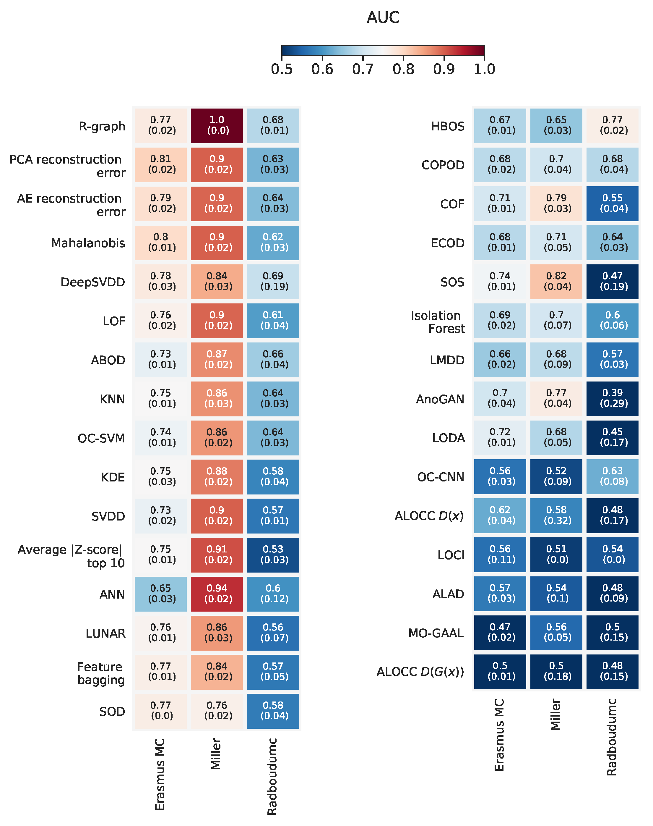
3.1. Performance Differences across Methods
3.2. Performance Differences across Datasets
3.3. Clinical Relevance of Outlier Detection Methods on Detecting IEM Patients
4. Discussion
5. Conclusions
Author Contributions
Funding
Institutional Review Board Statement
Informed Consent Statement
Data Availability Statement
Conflicts of Interest
Abbreviations
| ANN | Artificial neural network |
| AUC | Area under the curve |
| CV | Cross-validation |
| GAN | Generative adversarial network |
| ROC | Receiver operating characteristic |
| IEM | Inborn error of metabolism |
| PCA | Principle component analysis |
| PC | Principle component |
| UHPLC | Ultra-high performance liquid chromatography |
Appendix A. Datasets
Appendix A.1. Erasmus MC Dataset
Appendix A.2. Miller Dataset
Appendix A.3. Radboudumc Dataset
Appendix B. Detailed Description of Outlier Detection Methods
Appendix B.1. Autoencoder
Appendix B.2. ANN Classifier
- Uncorrelated normal noise: outlier profiles were drawn from N(=0, ) with three different values for , namely 0.25, 0.5, and 1.
- Subspace perturbation: following the method described by [16], where outlier profiles were acquired by perturbing normal profiles as follows:
Appendix B.3. ALOCC
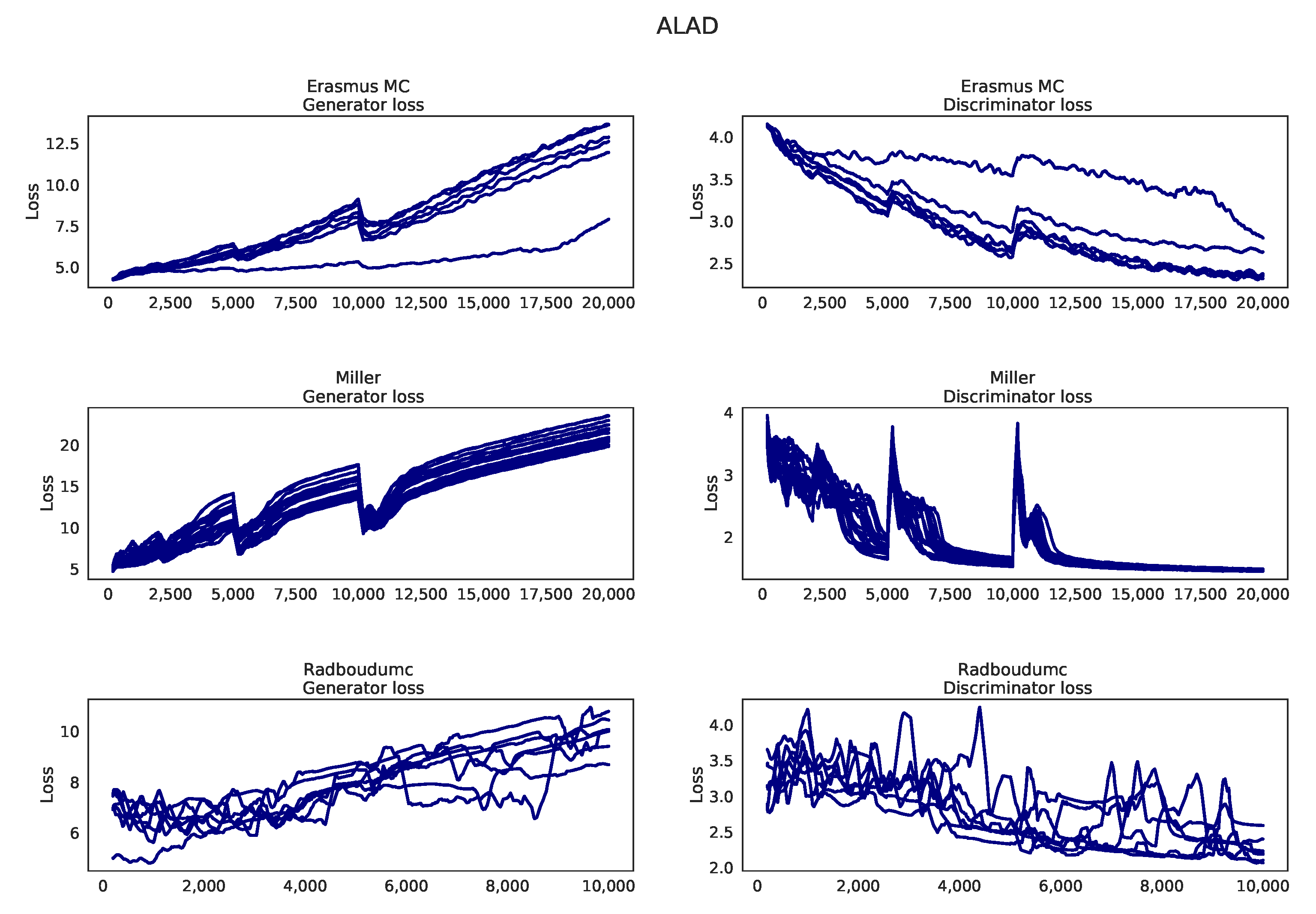
Appendix B.4. ALAD
Appendix B.5. AnoGAN
Appendix B.6. ABOD
Appendix Average of Top 10 Most Extreme Absolute Z-Scores
Appendix B.7. COPOD
Appendix B.8. COF
Appendix B.9. DeepSVDD
Appendix B.10. ECOD
Appendix B.11. HBOS
Appendix B.12. Isolation Forest
Appendix B.13. KDE
Appendix B.14. Feature Bagging
Appendix B.15. KNN
Appendix B.16. LMDD
Appendix B.17. LOCI
Appendix B.18. LODA
Appendix B.19. LOF
Appendix B.20. LUNAR
Appendix B.21. Mahalanobis
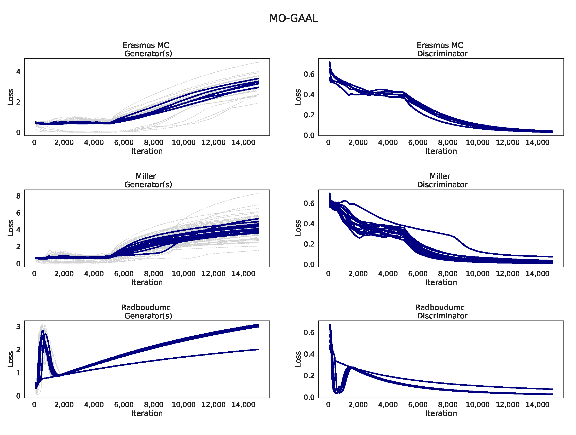
Appendix B.22. MO-GAAL
Appendix B.23. OC-SVM
Appendix B.24. OC-CNN
Appendix B.25. PCA reconstruction error
Appendix B.26. R-graph
Appendix B.27. SVDD
Appendix B.28. SOS
Appendix B.29. SOD

| Nr. | Name Method | Type | Summary of Working Principle | Distance Metric | Performs (Indirect) Dimensionality Reduction | Uses a Form of an (Artificial) Outlier Class for Training |
|---|---|---|---|---|---|---|
| 1 | AE reconstruction error | ANN | Reconstruction error between autoencoder reconstructed sample and input sample | l2 | Yes, latent space of the AE | |
| 2 | ALOCC | ANN (GAN) | GAN-based method, but replaces generator for an autoencoder. Outlier scores are obtained from discriminator that discriminates reconstructed samples from real samples. | Yes, latent space of the generator | ||
| 3 | ALAD | ANN (GAN) | GAN with multiple generator and discriminator networks. Outlier scores obtained from the l1 error between the activations in a hidden layer of the discriminator between reconstructed and input sample. | l1 | Yes, latent space of the generator | Generated samples from the generator |
| 4 | AnoGAN | ANN (GAN) | Reconstruction error between reconstructed and input sample after finding an approximate point in latent space of a query sample. | l1 | Yes, latent space of the generator | Generated samples from the generator |
| 5 | ANN classifier | ANN | ANN classifier that distinguishes noise from normal samples. | Yes | Random noise or subspace perturbation | |
| 6 | ABOD | Probabilistic | A comparison of the variance of angles between query sample and other samples in the dataset. Outlier samples are expected to have a lower (angle) variance. | No | ||
| 7 | Average of top 10 most extreme absolute Z-scores | Probabilistic | ||||
| 8 | COPOD | Probabilistic | Combines empirical cumulative distributions in a copula to estimate a ‘probability’ per sample. | No | ||
| 9 | COF | Compares the average chaining distance of a point with the average chaining distance of the k-nearest neighbors. | No | |||
| 10 | DeepSVDD | Support vector + ANN | Minimum volume of sphere containing majority of the normal samples using an ANN for non-linear mapping. | Yes | ||
| 11 | ECOD | Computes left- and right-tail univariate empirical cumulative distribution functions (ECDFs) per feature. ECOD uses the uni-variate ECDFs to estimate tail probabilities for the datapoint and aggregates these tail probabilities to a final outlier score. | No | |||
| 12 | HBOS | Density / proximity | Builds a histogram for each dimension and aggregates the results from each histogram into a single outlier score. | |||
| 13 | Isolation Forest | Ensemble | Number of splits needed to isolate a sample. | No | ||
| 14 | KDE | Density / proximity / Probabilistic | Density based on Gaussian kernel density approximation. | Depends on the used kernel | No | |
| 15 | Feature bagging | Ensemble | Ensemble of detectors that use a random subset of features. | |||
| 16 | KNN | Density / proximity | Mean, largest, or median distance of the k-nearest neighbors. | Euclidean, l1, l2 | No | |
| 17 | LMDD | |||||
| 18 | LOCI | Density / proximity | Compares the density of a sample with the density of its neighborhood. Density is measured by considering the multi-granularity deviation factor. | |||
| 19 | LODA | Ensemble | Using an ensemble of one-dimensional histograms by projecting the data to a (random) one-dimensional space. | Inconclusive | ||
| 20 | LOF | Density / proximity | Compares the average distance of a sample to its neighboring samples with the average distance of those samples with their neighborhood. | No | ||
| 21 | LUNAR | Graph + ANN | Uses a graph neural network (GNN), where the graph is determined from the local neighborhood of each sample. GNN is trained using an artificial outlier class. | Yes, depending on number of nodes in hidden layers | Subspace perturbation | |
| 22 | Mahalanobis | Density / proximity | Mahalanobis calculated from the estimated covariance matrix. | Mahalanobis | No | |
| 23 | MO-GAAL | ANN (GAN) | GAN with multiple generators to generate different parts of the normal data. | |||
| 24 | OC-SVM | Support vector | Finds a hyperplane that maximizes the distance of the normal data to the origin. | No | Origin is outlier class | |
| 25 | OC-CNN | ANN | ANN classifier that distinguishes noise from normal samples after feature extractor | Yes, latent space of the feature extractor (AE) | Random noise or subspace perturbation | |
| 26 | PCA reconstruction error | Density / proximity | Reconstruction error between input sample and reconstructed sample after projection to lower dimensional space from PCA. | l2 | Yes, PCA | |
| 27 | R-graph | Graph | Represents each samples as a linear combination of other samples, using a Markov process to propagate scores though the graph. | Projection in a (lower) subspace | ||
| 28 | SVDD | Support vector | Minimum volume of sphere containing majority of the normal samples (using a kernel). | |||
| 29 | SOS | Graph | Euclidean | |||
| 30 | SOD | Each sample’s outlierness is evaluated in a relevant subspace. | Projection in a (lower) subspace |
Appendix C. Optimal Settings for Each Dataset and Outlier Detection Method
| Method | Setting | Erasmus MC | Miller | Radboudumc |
|---|---|---|---|---|
| ALAD | epochs | 100 | 10,000 | 500 |
| ALAD | latent_dim | 4 | 3 | 4 |
| ALOCC D(x) | epochs | 100 | 5000 | 100 |
| ALOCC G(D(x)) | epochs | 2000 | 500 | 1000 |
| ANN | bias | False | False | True |
| ANN | epochs | 500 | 2000 | 5000 |
| ANN | noise | normal | subspace_ perturbation | normal |
| ANN | std | 1 | 1 | 0.25 |
| AnoGAN | epochs | 2000 | 100 | 2000 |
| AnoGAN | latent_dim | 3 | 3 | 3 |
| DeepSVDD | epochs | 10 | 1000 | 1000 |
| HBOS | alpha | 0.1 | 0.1 | 0.5 |
| HBOS | n_bins | 100 | 50 | 250 |
| Isolation Forest | n_estimators | 500 | 500 | 500 |
| KDE | bandwidth | 0.25 | 0.25 | 0.5 |
| KNN | distance | euclidean | euclidean | l1 |
| KNN | method | mean | mean | mean |
| KNN | n_neighbors_frac | 0.05 | 0.05 | 0.1 |
| LOCI | alpha | 0.1 | 0.5 | 0.5 |
| LOCI | k | 1 | 1 | 2 |
| LODA | n_bins | 50 | 10 | auto |
| LODA | n_random_cuts | 500 | 500 | 100 |
| LOF | n_neighbors_frac | 0.05 | 0.1 | 0.05 |
| LUNAR | n_neighbors_frac | 0.1 | 0.1 | 0.1 |
| MO-GAAL | k | 5 | 5 | 5 |
| OC-CNN | bias | True | True | True |
| OC-CNN | epochs | 5000 | 15000 | 5000 |
| OC-CNN | noise | uniform | normal | uniform |
| OC-CNN | sigma | 0.5 | 1 | 0.5 |
| OC-SVM | kernel | rbf | rbf | linear |
| PCA reconstruction error | n_components | 50 | 25 | 100 |
| R-graph | gamma | 100 | 100 | 50 |
| R-graph | n_nonzero_frac | 0.05 | 0.25 | 0.25 |
| R-graph | steps | 100 | 25 | 10 |
| SOD | n_neighbors_frac | 0.05 | 0.05 | 0.25 |
| SOS | perplexity_frac | 0.5 | 0.25 | 0.5 |
| SVDD | C | 2 | 1 | 2 |
| SVDD | kernel | rbf | linear | linear |
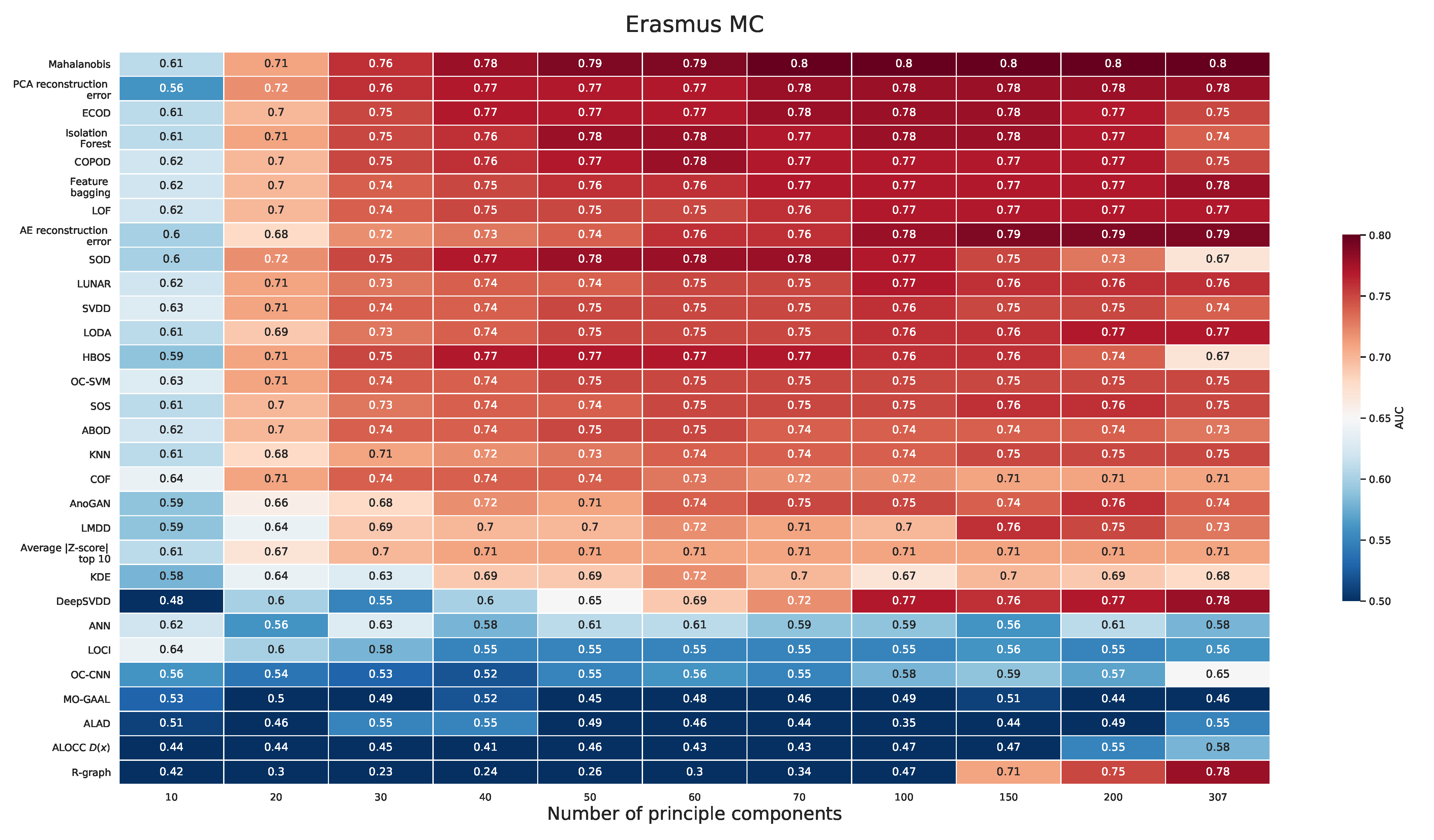
Appendix D. PCA Prior to Applying the Outlier Detection Method (Erasmus MC)

| Method | Setting | Value |
|---|---|---|
| OCSVM | kernel | rbf |
| SVDD | C | 1 |
| SVDD | kernel | rbf |
| PCA reconstruction error | n_components | 9 |
| ALOCC D(x) | epochs | 10,000 |
| OC-CNN | bias | False |
| OC-CNN | epochs | 10,000 |
| OC-CNN | noise | uniform |
| OC-CNN | sigma | 0.1 |
| ANN | bias | False |
| ANN | epochs | 10,000 |
| ANN | noise | normal |
| ANN | std | 0.25 |
| LODA | n_bins | 50 |
| LODA | n_random_cuts | 500 |
| LOCI | alpha | 0.1 |
| LOCI | k | 1 |
| R-graph | gamma | 100 |
| R-graph | n_nonzero_frac | 0.05 |
| R-graph | steps | 100 |
| MO-GAAL | k | 5 |
| HBOS | alpha | 0.1 |
| HBOS | n_bins | 100 |
| DeepSVDD | epochs | 10 |
| SOS | perplexity_frac | 0.5 |
| SOD | n_neighbors_frac | 0.1 |
| Isolation Forest | n_estimators | 500 |
| LOF | n_neighbors_frac | 0.05 |
| KNN | distance | euclidean |
| KNN | method | largest |
| KNN | n_neighbors_frac | 0.05 |
| KDE | bandwidth | 0.25 |
| LUNAR | n_neighbors_frac | 0.1 |
| AnoGAN | epochs | 10,000 |
| AnoGAN | latent_dim | 3 |
| ALAD | epochs | 10,000 |
| ALAD | latent_dim | 3 |
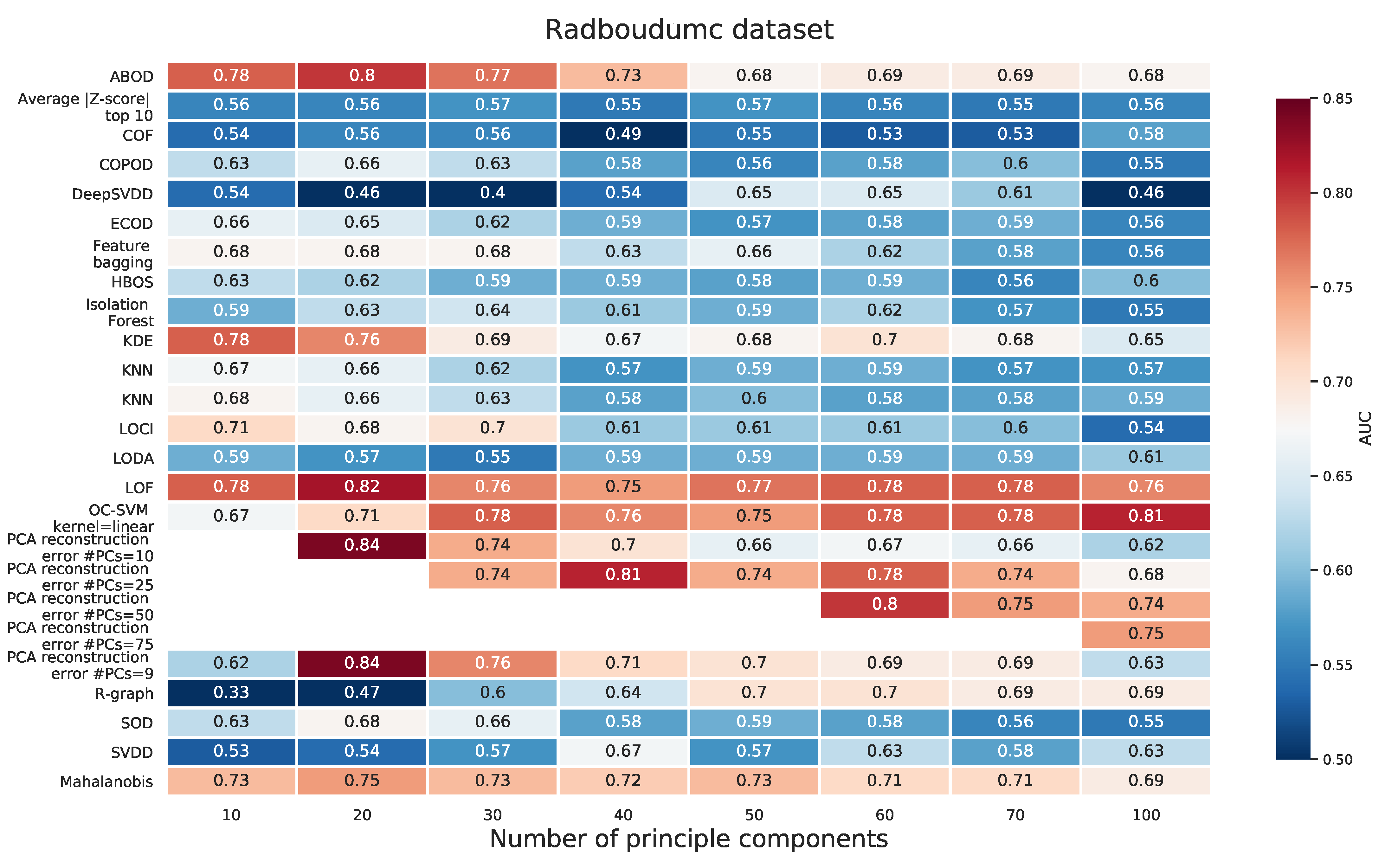
Appendix E. PCA Prior to Applying the Outlier Detection Method for Radboudumc Dataset


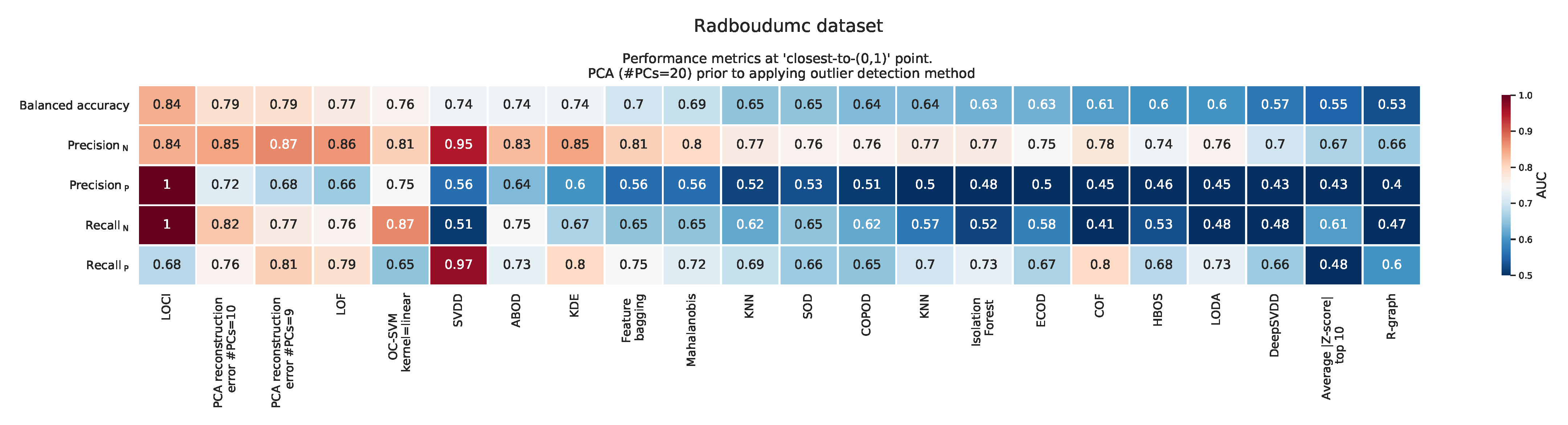
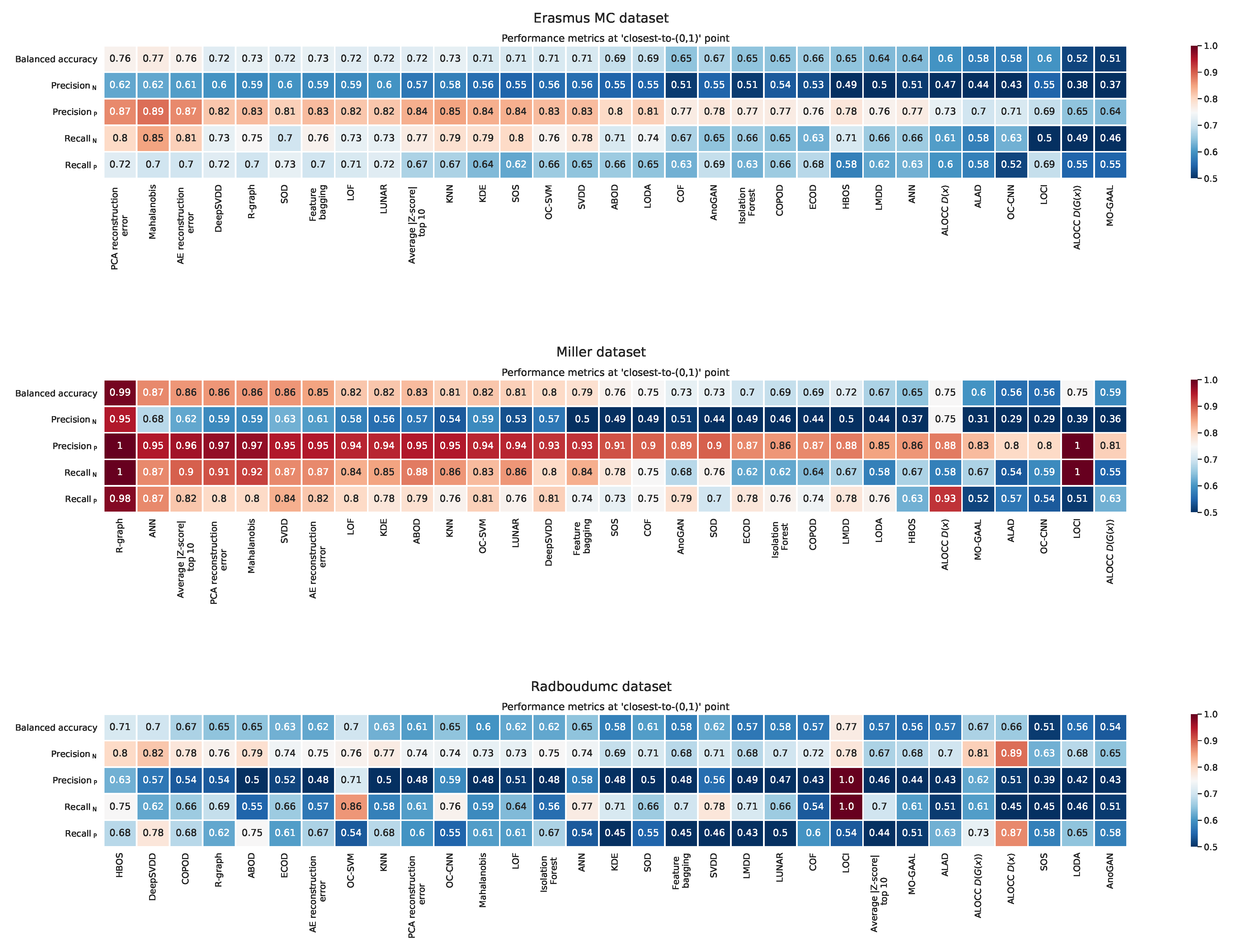
Appendix F. Balanced Accuracy, Recall, and Precision at the ‘Closest to the (0,1)’ Point

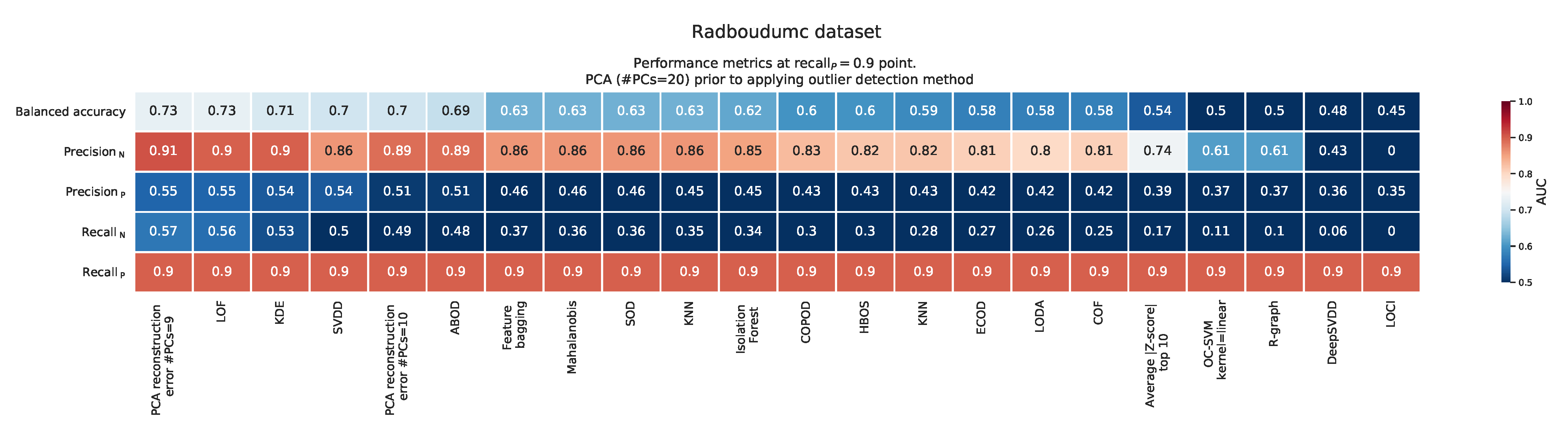
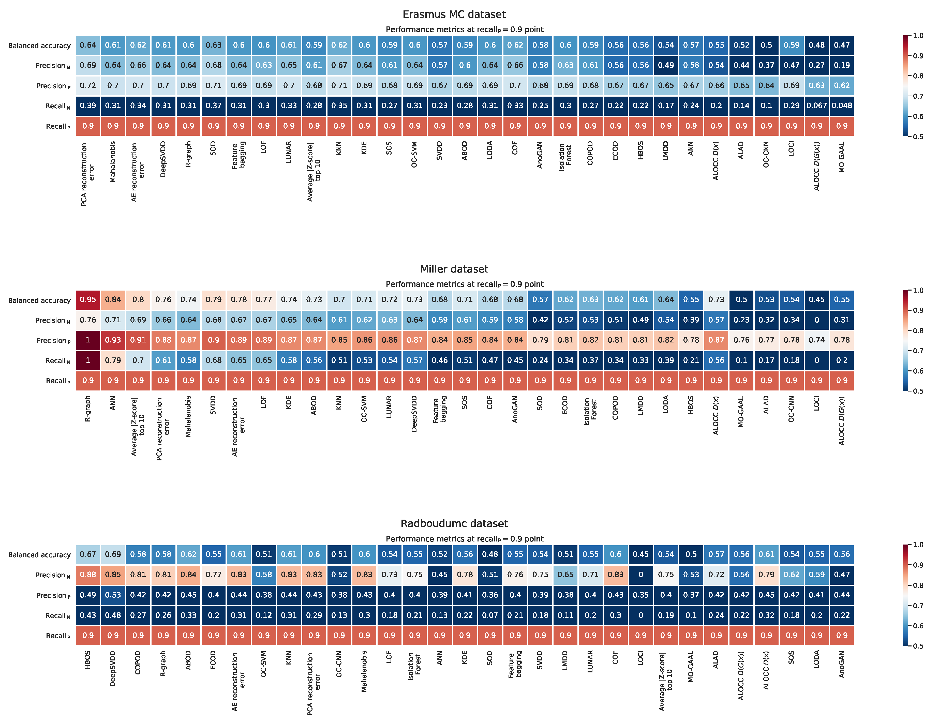
Appendix G. Balanced Accuracy, Recall, and Precision at the ‘Recall P = 0.9’ Point

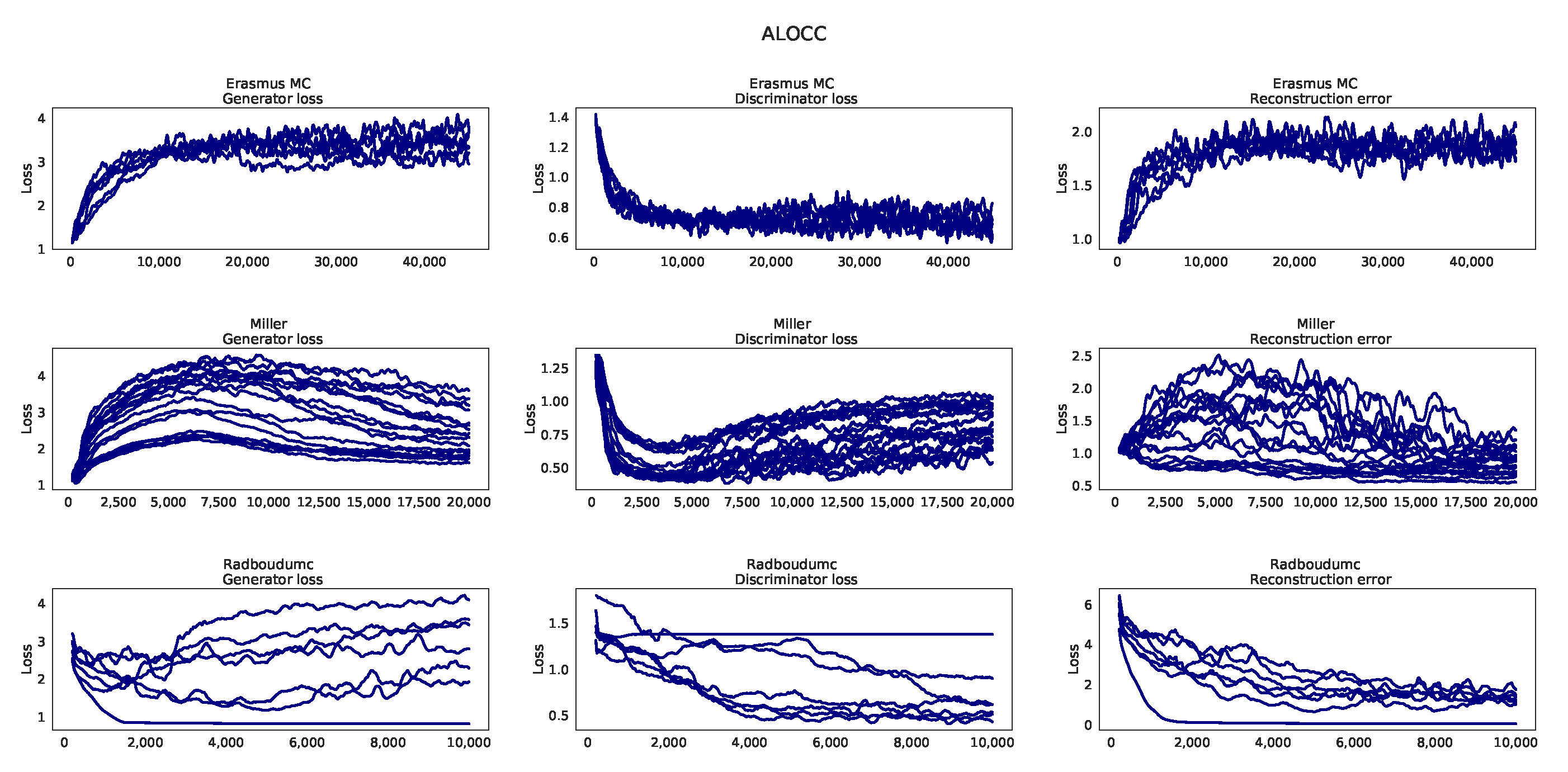
Appendix H. Learning Curves ALOCC

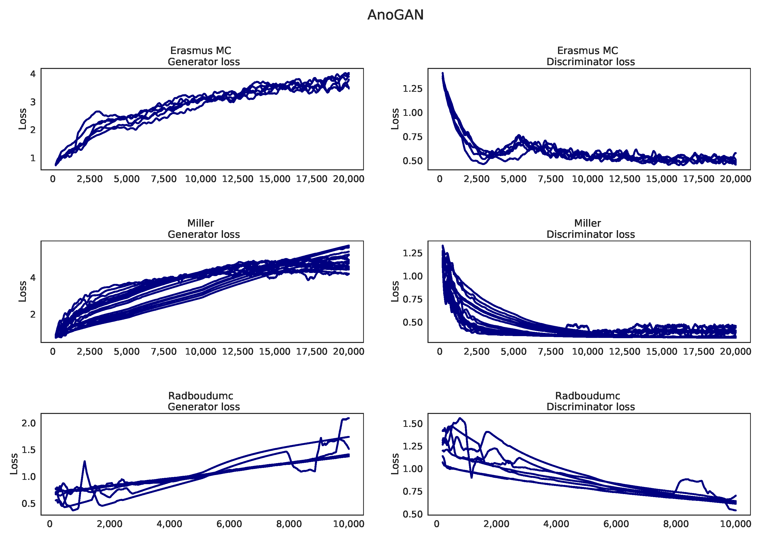
Appendix I. Learning Curves AnoGAN

Appendix J. Learning Curves ALAD

Appendix K. Learning curves MO-GAAL

Appendix L. Overview with Standard Deviations on AUC

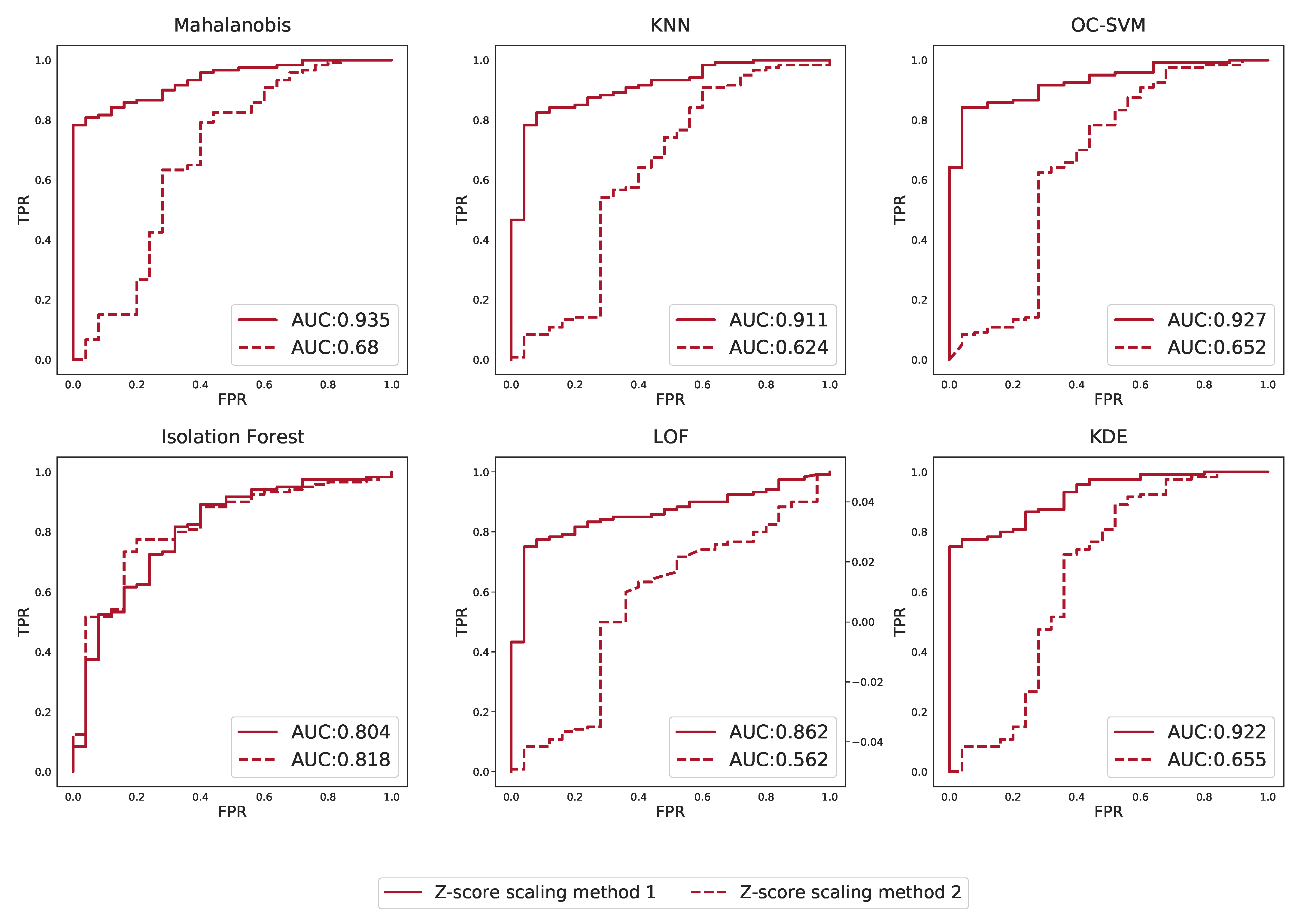
Appendix M. Effect of Scaling Based on Different Groups on Outlier Detection Performance

References
- Miller, M.J.; Kennedy, A.D.; Eckhart, A.D.; Burrage, L.C.; Wulff, J.E.; Miller, L.A.D.; Milburn, M.V.; Ryals, J.A.; Beaudet, A.L.; Sun, Q.; et al. Untargeted metabolomic analysis for the clinical screening of inborn errors of metabolism. J. Inherit. Metab. Dis. 2015, 38, 1029–1039. [Google Scholar] [CrossRef] [PubMed]
- Coene, K.L.M.; Kluijtmans, L.A.J.; Heeft, E.v.; Engelke, U.F.H.; de Boer, S.; Hoegen, B.; Kwast, H.J.T.; Vorst, M.v.d.; Huigen, M.C.D.G.; Keularts, I.M.L.W.; et al. Next-generation metabolic screening: Targeted and untargeted metabolomics for the diagnosis of inborn errors of metabolism in individual patients. J. Inherit. Metab. Dis. 2018, 41, 337–353. [Google Scholar] [CrossRef] [PubMed]
- Bonte, R.; Bongaerts, M.; Demirdas, S.; Langendonk, J.G.; Huidekoper, H.H.; Williams, M.; Onkenhout, W.; Jacobs, E.H.; Blom, H.J.; Ruijter, G.J.G. Untargeted metabolomics-based screening method for inborn errors of metabolism using semi-automatic sample preparation with an UHPLC- orbitrap-MS platform. Metabolites 2019, 9, 289. [Google Scholar] [CrossRef]
- Almontashiri, N.A.M.; Zha, L.; Young, K.; Law, T.; Kellogg, M.D.; Bodamer, O.A.; Peake, R.W.A. Clinical validation of targeted and untargeted metabolomics testing for genetic disorders: A 3 year comparative study. Sci. Rep. 2020, 10, 9382. [Google Scholar] [CrossRef]
- Donti, T.R.; Cappuccio, G.; Hubert, L.; Neira, J.; Atwal, P.S.; Miller, M.J.; Cardon, A.L.; Sutton, V.R.; Porter, B.E.; Baumer, F.M.; et al. Diagnosis of adenylosuccinate lyase deficiency by metabolomic profiling in plasma reveals a phenotypic spectrum. Mol. Genet. Metab. Rep. 2016, 8, 61–66. [Google Scholar] [CrossRef] [PubMed]
- Hoegen, B.; Zammit, A.; Gerritsen, A.; Engelke, U.F.H.; Castelein, S.; Vorst, M.v.; Kluijtmans, L.A.J.; Huigen, M.C.D.G.; Wevers, R.A.; Gool, A.J.v.; et al. Metabolomics-based screening of inborn errors of metabolism: Enhancing clinical application with a robust computational pipeline. Metabolites 2021, 11, 568. [Google Scholar] [CrossRef]
- Janeckova, H.; Kalivodova, A.; Najdekr, L.; Friedecky, D.; Hron, K.; Bruheim, P.; Adam, T. Untargeted metabolomic analysis of urine samples in the diagnosis of some inherited metabolic disorders. Biomed. Pap. 2015, 159, 582–585. [Google Scholar] [CrossRef] [PubMed]
- Kennedy, A.D.; Pappan, K.L.; Donti, T.R.; Evans, A.M.; Wulff, J.E.; Miller, L.A.D.; Sutton, V.R.; Sun, Q.; Miller, M.J.; Elsea, S.H. Elucidation of the complex metabolic profile of cerebrospinal fluid using an untargeted biochemical profiling assay. Mol. Genet. Metab. 2017, 121, 83–90. [Google Scholar] [CrossRef]
- Sindelar, M.; Dyke, J.P.; Deeb, R.S.; Sondhi, D.; Kaminsky, S.M.; Kosofsky, B.E.; Ballon, D.J.; Crystal, R.G.; Gross, S.S. Untargeted metabolite profiling of cerebrospinal fluid uncovers biomarkers for severity of late infantile neuronal ceroid lipofuscinosis (CLN2, batten disease). Sci. Rep. 2018, 8, 15229. [Google Scholar] [CrossRef]
- Tebani, A.; Abily-Donval, L.; Schmitz-Afonso, I.; Piraud, M.; Ausseil, J.; Zerimech, F.; Pilon, C.; Pereira, T.; Marret, S.; Afonso, C.; et al. Analysis of mucopolysaccharidosis type VI through integrative functional metabolomics. Int. J. Mol. Sci. 2019, 20, 446. [Google Scholar] [CrossRef]
- Wangler, M.F.; Hubert, L.; Donti, T.R.; Ventura, M.J.; Miller, M.J.; Braverman, N.; Gawron, K.; Bose, M.; Moser, A.B.; Jones, R.O.; et al. A metabolomic map of zellweger spectrum disorders reveals novel disease biomarkers. Genet. Med. 2018, 20, 1274–1283. [Google Scholar] [CrossRef] [PubMed]
- Wikoff, W.R.; Gangoiti, J.A.; Barshop, B.A.; Siuzdak, G. Metabolomics identifies perturbations in human disorders of propionate metabolism. Clin. Chem. 2007, 53, 2169–2176. [Google Scholar] [CrossRef] [PubMed]
- Engel, J.; Blanchet, L.; Engelke, U.F.H.; Wevers, R.A.; Buydens, L.M.C. Towards the disease biomarker in an individual patient using statistical health monitoring. PLoS ONE 2014, 9, e92452. [Google Scholar] [CrossRef] [PubMed]
- Brini, A.; Avagyan, V.; de Vos, R.C.H.; Vossen, J.H.; Heuvel, E.R.v.; Engel, J. Improved one-class modeling of high-dimensional metabolomics data via eigenvalue-shrinkage. Metabolites 2021, 11, 237. [Google Scholar] [CrossRef] [PubMed]
- Breunig, M.M.; Kriegel, H.; Ng, R.T.; Sander, J. LOF. In Proceedings of the 2000 ACM SIGMOD International Conference on Management of Data—SIGMOD ’00, Dallas, TX, USA, 16–18 May 2000; ACM Press: New York, NY, USA, 2000. [Google Scholar]
- Goodge, A.; Hooi, B.; Ng, S.; Ng, W.S. Lunar: Unifying local outlier detection methods via graph neural networks. In Proceedings of the AAAI Conference on Artificial Intelligence, virtually, 22 February–1 March 2022. [Google Scholar]
- Schölkopf, B.; Platt, J.C.; Shawe-Taylor, J.; Smola, A.J.; Williamson, R.C. Estimating the support of a high-dimensional distribution. Neural Comput. 2001, 13, 1443–1471. [Google Scholar] [CrossRef] [PubMed]
- David, M.J. Tax and Robert P.W. Duin. Support vector data description. Mach. Learn. 2004, 54, 45–66. [Google Scholar]
- Janssens, E.P.J.; Huszár, F.; van den Herik, J. Stochastic outlier selection. In Technical Report, Technical Report TiCC TR 2012–001; Tilburg University, Tilburg Center for Cognition and Communication: Tilburg, The Netherlands, 2012. [Google Scholar]
- You, C.; Robinson, D.P.; Vidal, R. Provable self-representation based outlier detection in a union of subspaces. In Proceedings of the IEEE Conference on Computer Vision and Pattern Recognition (CVPR), Honolulu, HI, USA, 21–26 July 2017. [Google Scholar]
- Liu, F.T.; Ting, K.M.; Zhou, Z. Isolation forest. In Proceedings of the 2008 Eighth IEEE International Conference on Data Mining, Pisa, Italy, 15–19 December 2008. [Google Scholar]
- Oza, P.; Patel, V.M. One-class convolutional neural network. IEEE Signal Process. Lett. 2019, 26, 277–281. [Google Scholar] [CrossRef]
- Ruff, L.; Vandermeulen, R.; Goernitz, N.; Deecke, L.; Siddiqui, S.A.; Binder, A.; Müller, E.; Kloft, M. Deep one-class classification. In Proceedings of the 35th International Conference on Machine Learning, Stockholm, Sweden, 10–15 July 2018; Dy, J., Krause, A., Eds.; Volume 80, pp. 4393–4402. [Google Scholar]
- Sabokrou, M.; Khalooei, M.; Fathy, M.; Adeli, E. Adversarially learned one-class classifier for novelty detection. In Proceedings of the 2018 IEEE/CVF Conference on Computer Vision and Pattern Recognition, Salt Lake City, UT, USA, 18–23 June 2018. [Google Scholar]
- Schlegl, T.; Seeböck, P.; Waldstein, S.M.; Schmidt-Erfurth, U.; Langs, G. Unsupervised anomaly detection with generative adversarial networks to guide marker discovery. In Lecture Notes in Computer Science; Springer International Publishing: New York, NY, USA, 2017; pp. 146–157. [Google Scholar]
- Liu, Y.; Li, Z.; Zhou, C.; Jiang, Y.; Sun, J.; Wang, M.; He, X. Generative adversarial active learning for unsupervised outlier detection. IEEE Trans. Knowl. Data Eng. 2020, 32, 1517–1528. [Google Scholar] [CrossRef]
- Zenati, H.; Romain, M.; Foo, C.; Lecouat, B.; Chandrasekhar, V.R. Adversarially learned anomaly detection. In Proceedings of the 2018 IEEE International Conference on Data Mining (ICDM), Singapore, 17–20 November 2018; pp. 727–736. [Google Scholar]
- Goodfellow, I.J.; Pouget-Abadie, J.; Mirza, M.; Xu, B.; Warde-Farley, D.; Ozair, S.; Courville, A.C.; Bengio, Y. Generative adversarial nets. In Proceedings of the 27th International Conference on Neural Information Processing Systems, Montreal, QC, Canada, 8–13 December 2014. [Google Scholar]
- Han, S.; Hu, X.; Huang, H.; Jiang, M.; Zhao, Y. Adbench: Anomaly detection benchmark. arXiv 2022, arXiv:abs/2206.09426. [Google Scholar] [CrossRef]
- Campos, G.O.; Zimek, A.; Sander, J.; Campello, R.J.G.B.; Micenková, B.; Schubert, E.; Assent, I.; Houle, M.E. On the evaluation of unsupervised outlier detection: Measures, datasets, and an empirical study. Data Min. Knowl. Discov. 2016, 30, 891–927. [Google Scholar] [CrossRef]
- Pedregosa, F.; Varoquaux, G.; Gramfort, A.; Michel, V.; Thirion, B.; Grisel, O.; Blondel, M.; Prettenhofer, P.; Weiss, R.; Dubourg, V.; et al. Scikit-learn: Machine learning in python. J. Mach. Learn. Res. 2011, 12, 2825–2830. [Google Scholar]
- Zhao, Y.; Nasrullah, Z.; Li, Z. Pyod: A python toolbox for scalable outlier detection. J. Mach. Learn. Res. 2019, 20, 1–7. [Google Scholar]
- Smith, C.A.; Want, E.J.; O’Maille, G.; Abagyan, R.; Siuzdak, G. XCMS: Processing mass spectrometry data for metabolite profiling using nonlinear peak alignment, matching, and identification. Anal. Chem. 2006, 78, 779–787. [Google Scholar] [CrossRef] [PubMed]
- Goodfellow, I. Nips 2016 tutorial: Generative adversarial networks. arXiv 2017, arXiv:1701.00160. [Google Scholar]
- Bongaerts, M.; Bonte, R.; Demirdas, S.; Jacobs, E.H.; Oussoren, E.; Ploeg, A.T.v.; Wagenmakers, M.A.E.M.; Hofstra, R.M.W.; Blom, H.J.; Reinders, M.J.T.; et al. Using out-of-batch reference populations to improve untargeted metabolomics for screening inborn errors of metabolism. Metabolites 2020, 11, 8. [Google Scholar] [CrossRef]
- Brunius, C.; Shi, L.; Landberg, R. Large-scale untargeted lc-ms metabolomics data correction using between-batch feature alignment and cluster-based within-batch signal intensity drift correction. Metabolomics 2016, 12, 173. [Google Scholar] [CrossRef]
- Abadi, M.; Agarwal, A.; Barham, P.; Brevdo, E.; Chen, Z.; Citro, C.; Corrado, G.S.; Davis, A.; Dean, J.; Devin, M.; et al. TensorFlow: Large-Scale Machine Learning on Heterogeneous Systems. 2015. Available online: tensorflow.org (accessed on 26 June 2022).
- Chollet, F. Keras. 2015. Available online: https://keras.io (accessed on 26 June 2022).
- Kriegel, H.; Schubert, M.; Zimek, A. Angle-based outlier detection in high-dimensional data. In Proceedings of the 14th ACM SIGKDD International Conference on Knowledge Discovery and Data Mining, KDD ’08, Las Vegas, NA, USA, 24–27 August 2008; Association for Computing Machinery: New York, NY, USA, 2008; pp. 444–452. [Google Scholar]
- Li, Z.; Zhao, Y.; Botta, N.; Ionescu, C.; Hu, X. COPOD: Copula-Based Outlier Detection. In Proceedings of the 2020 IEEE International Conference On Data Mining (ICDM), Sorrento, Italy, 17–20 November 2020; pp. 1118–1123. [Google Scholar]
- Tang, J.; Chen, Z.; Fu, A.W.; Cheung, D.W. Enhancing effectiveness of outlier detections for low density patterns. In Proceedings of the 6th Pacific-Asia Conference on Advances in Knowledge Discovery and Data Mining, PAKDD ’02, Taipei, Taiwan, 6–8 May 2002; Springer: Berlin/Heidelberg, Germany, 2002; pp. 535–548. [Google Scholar]
- Li, Z.; Zhao, Y.; Hu, X.; Botta, N.; Ionescu, C.; Chen, G. ECOD: Unsupervised outlier detection using empirical cumulative distribution functions. IEEE Trans. Knowl. Data Eng. 2022. [Google Scholar] [CrossRef]
- Goldstein, M.; Dengel, A.R. Histogram-based outlier score (hbos): A fast unsupervised anomaly detection algorithm. In Proceedings of the Poster and Demo Track of the 35th German Conference on Artificial Intelligence (KI-2012), Saarbrücken, Germany, 24–27 September 2012; pp. 59–63. [Google Scholar]
- Lazarevic, A.; Kumar, V. Feature bagging for outlier detection. Proceeding of the Eleventh ACM SIGKDD International Conference on Knowledge Discovery in Data Mining—KDD ’05, Chicago, IL, USA, 21–24 August 2005; ACM Press: New York, NY, USA, 2005. [Google Scholar]
- Arning, A.; Agrawal, R.; Raghavan, P. A linear method for deviation detection in large databases. In Proceedings of the Second International Conference on Knowledge Discovery and Data Mining, Portland, OR, USA, 2–4 August 1996. [Google Scholar]
- Papadimitriou, S.; Kitagawa, H.; Gibbons, P.B.; Faloutsos, C. Loci: Fast outlier detection using the local correlation integral. Proceedings 19th International Conference on Data Engineering (Cat. No.03CH37405), Bangalore, India, 5–8 March 2003; pp. 315–326. [Google Scholar]
- Pevný, T. Loda: Lightweight on-line detector of anomalies. Mach. Learn. 2015, 102, 275–304. [Google Scholar] [CrossRef]
- Kriegel, H.; Kröger, P.; Schubert, E.; Zimek, A. Outlier detection in axis-parallel subspaces of high dimensional data. In Advances in Knowledge Discovery and Data Mining; Springer: Berlin/Heidelberg, Germany, 2009; pp. 831–838. [Google Scholar]


| Dataset | Experimental Set-Up | Tissue Type | # Experimental Batches | # Normal Samples | # Abnormal Samples | # Different IEM | Receiving Treatment | # Features |
|---|---|---|---|---|---|---|---|---|
| Erasmuc MC [3] | LC-MS(+) | Blood plasma | 25 | 552 | 122 | 62 | 50% | 307 |
| Miller et al. [1] | GS-MS & LC-MS(+/−) | Blood plasma | 1 * | 70 | 120 | 21 | >50% ** | 661 † |
| Radboudumc [2] | LC-MS(+) | Blood plasma | 12 | 123 | 41 | 28 | ≈75% | 6362 |
Disclaimer/Publisher’s Note: The statements, opinions and data contained in all publications are solely those of the individual author(s) and contributor(s) and not of MDPI and/or the editor(s). MDPI and/or the editor(s) disclaim responsibility for any injury to people or property resulting from any ideas, methods, instructions or products referred to in the content. |
© 2023 by the authors. Licensee MDPI, Basel, Switzerland. This article is an open access article distributed under the terms and conditions of the Creative Commons Attribution (CC BY) license (https://creativecommons.org/licenses/by/4.0/).
Share and Cite
Bongaerts, M.; Kulkarni, P.; Zammit, A.; Bonte, R.; Kluijtmans, L.A.J.; Blom, H.J.; Engelke, U.F.H.; Tax, D.M.J.; Ruijter, G.J.G.; Reinders, M.J.T. Benchmarking Outlier Detection Methods for Detecting IEM Patients in Untargeted Metabolomics Data. Metabolites 2023, 13, 97. https://doi.org/10.3390/metabo13010097
Bongaerts M, Kulkarni P, Zammit A, Bonte R, Kluijtmans LAJ, Blom HJ, Engelke UFH, Tax DMJ, Ruijter GJG, Reinders MJT. Benchmarking Outlier Detection Methods for Detecting IEM Patients in Untargeted Metabolomics Data. Metabolites. 2023; 13(1):97. https://doi.org/10.3390/metabo13010097
Chicago/Turabian StyleBongaerts, Michiel, Purva Kulkarni, Alan Zammit, Ramon Bonte, Leo A. J. Kluijtmans, Henk J. Blom, Udo F. H. Engelke, David M. J. Tax, George J. G. Ruijter, and Marcel J. T. Reinders. 2023. "Benchmarking Outlier Detection Methods for Detecting IEM Patients in Untargeted Metabolomics Data" Metabolites 13, no. 1: 97. https://doi.org/10.3390/metabo13010097
APA StyleBongaerts, M., Kulkarni, P., Zammit, A., Bonte, R., Kluijtmans, L. A. J., Blom, H. J., Engelke, U. F. H., Tax, D. M. J., Ruijter, G. J. G., & Reinders, M. J. T. (2023). Benchmarking Outlier Detection Methods for Detecting IEM Patients in Untargeted Metabolomics Data. Metabolites, 13(1), 97. https://doi.org/10.3390/metabo13010097