
Optimization of Imputation Strategies for High-Resolution Gas Chromatography–Mass Spectrometry (HR GC–MS) Metabolomics Data

 , ,
, ,  and
and 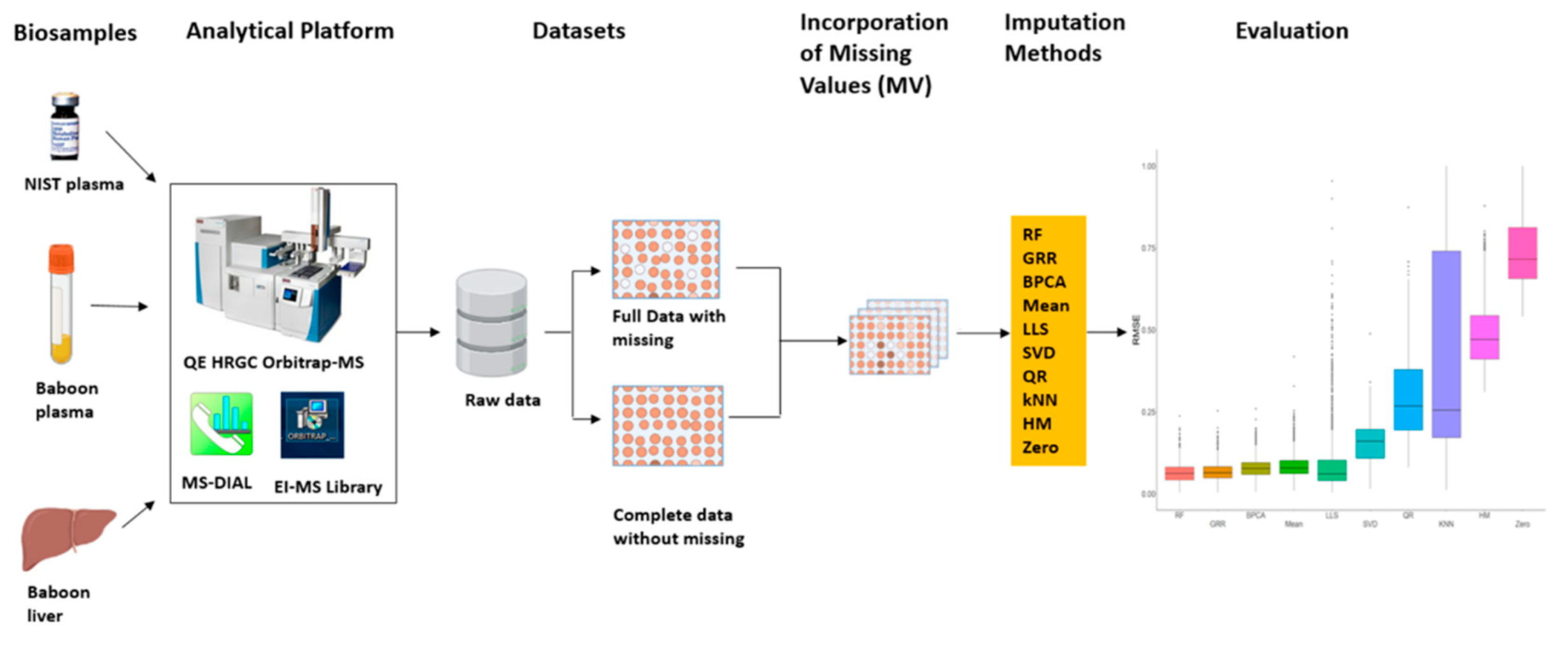
Abstract
1. Introduction
2. Results
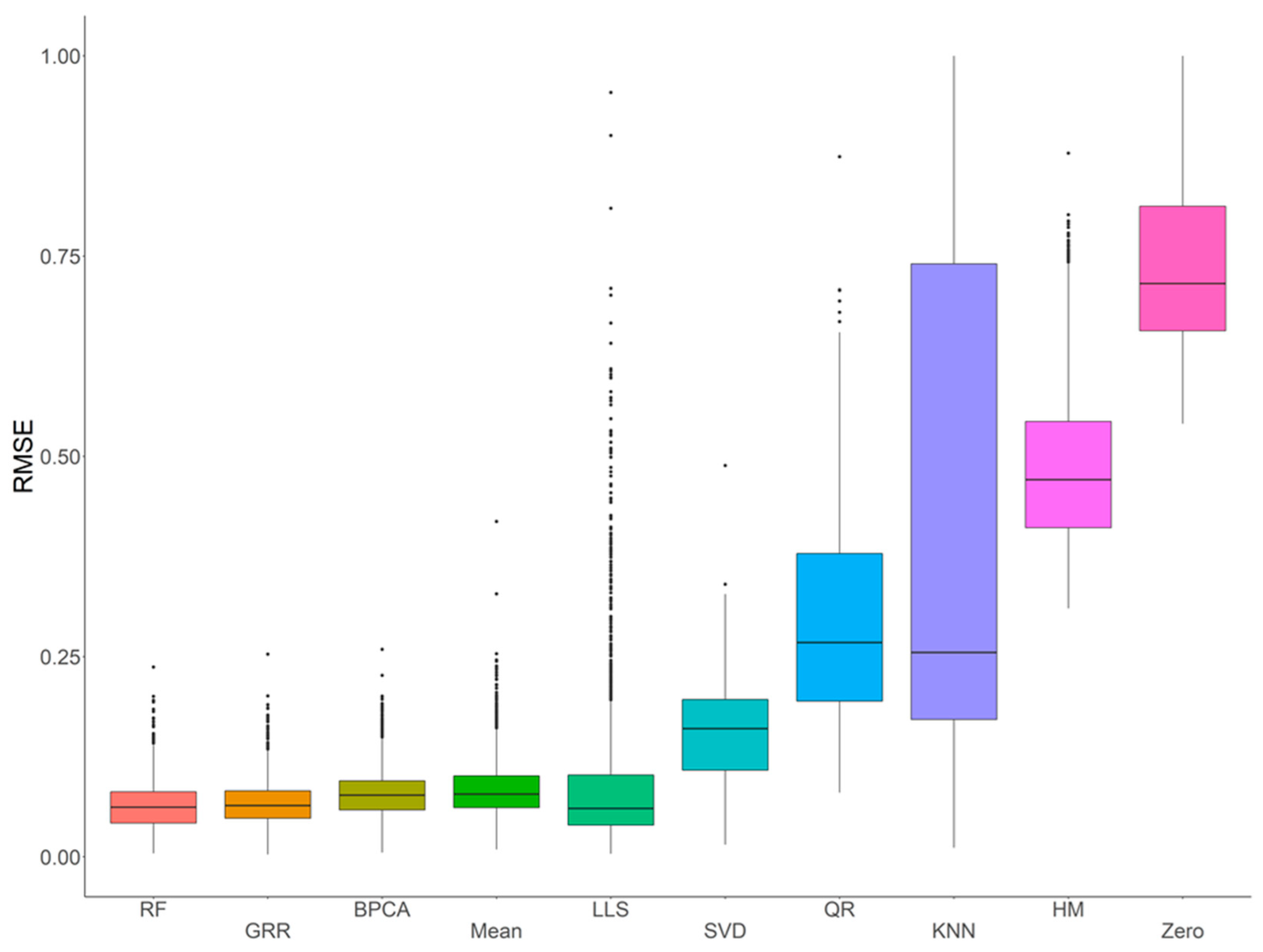
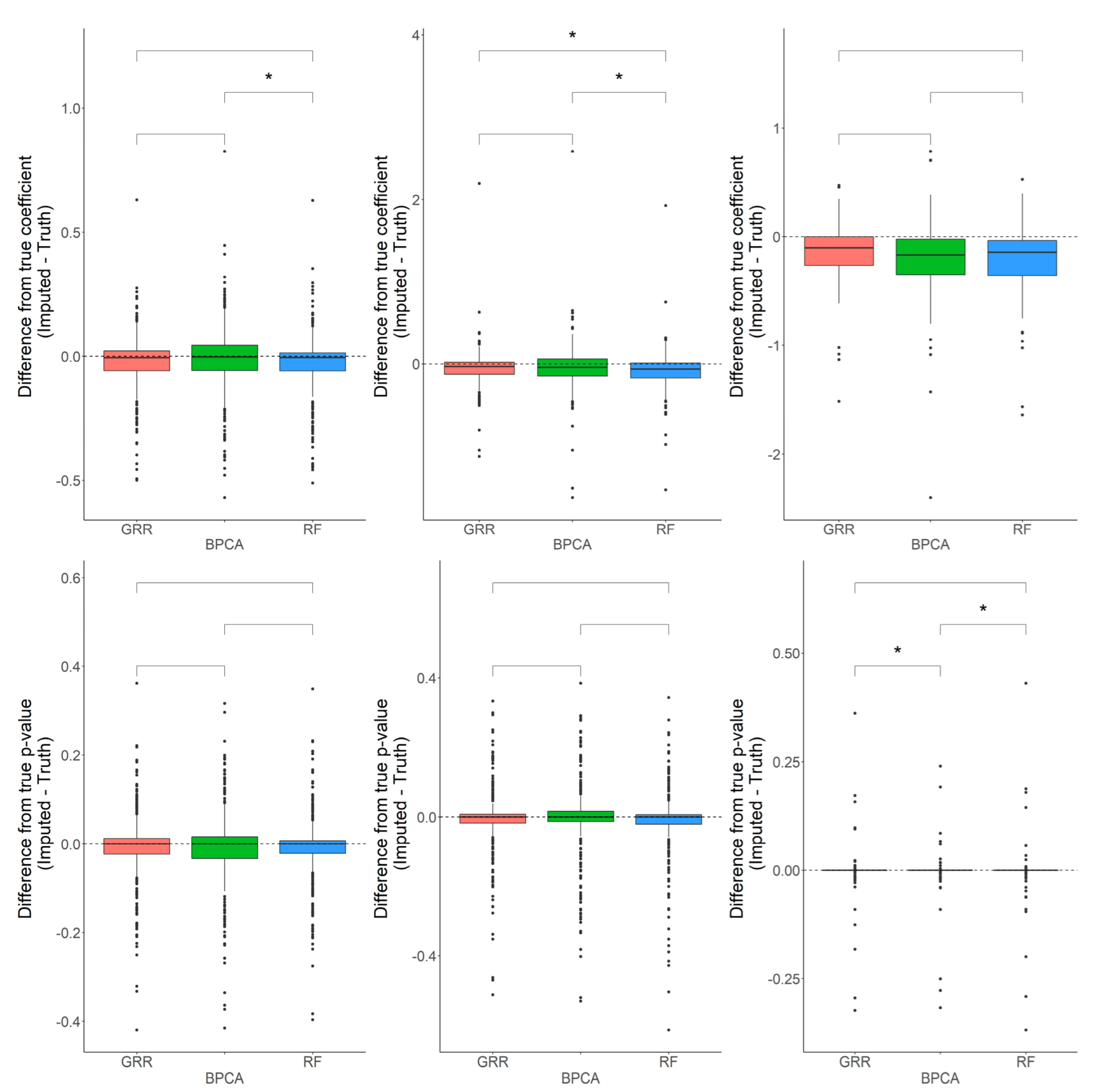
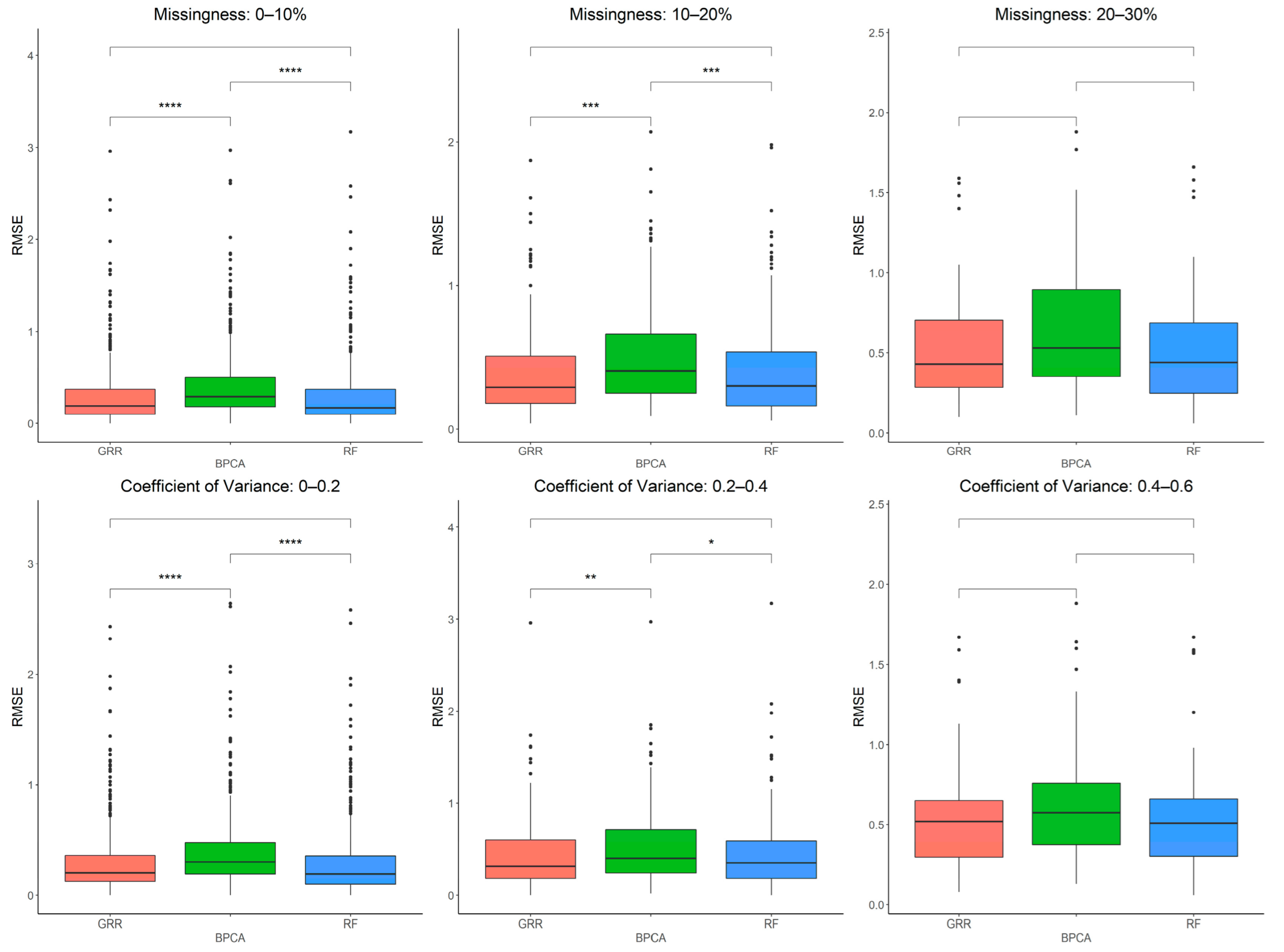
2.1. Missing Values Simulation and Imputation Evaluation Using HR GC–MS Metabolomics Data for Replicates of NIST Plasma
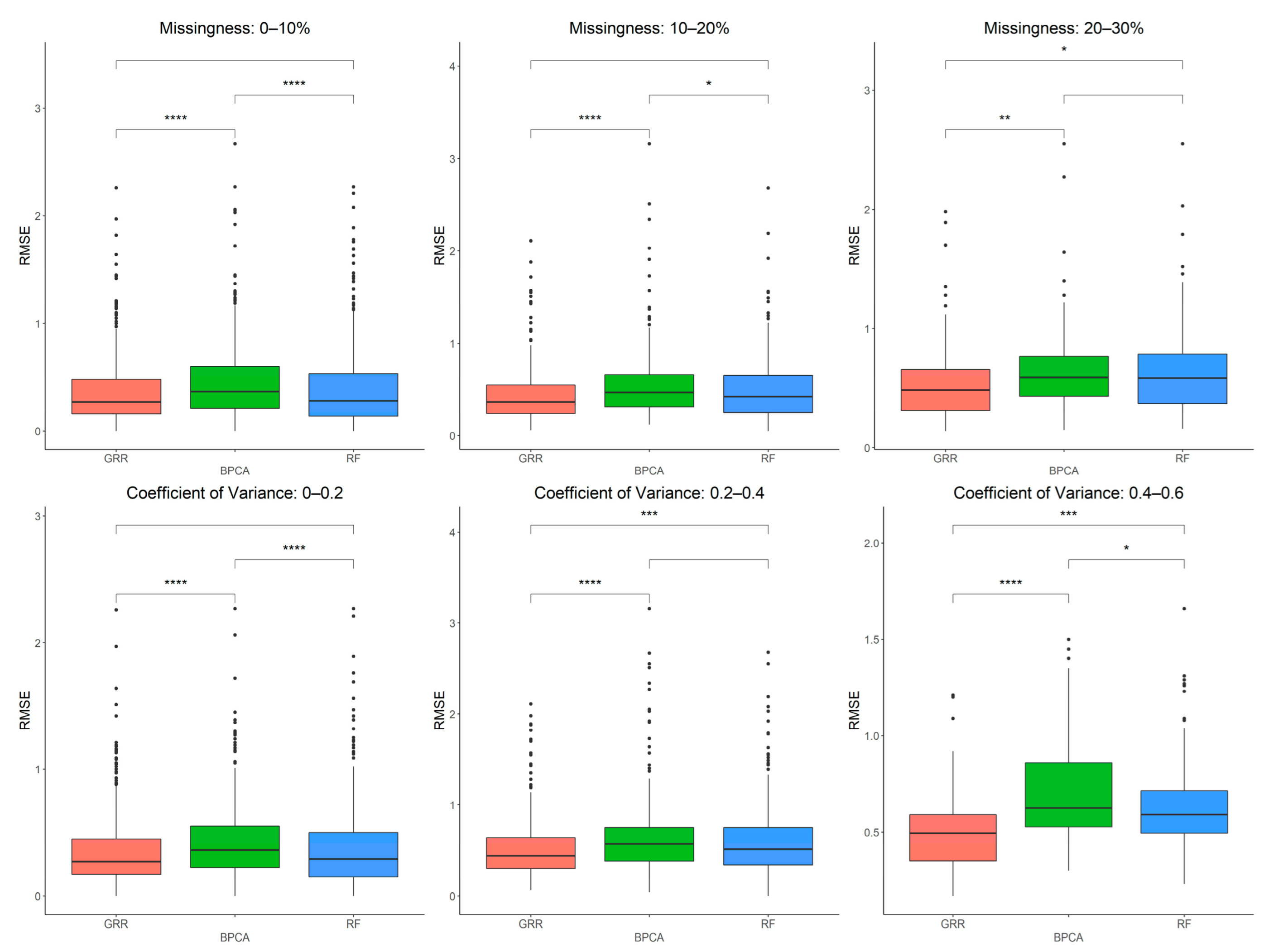
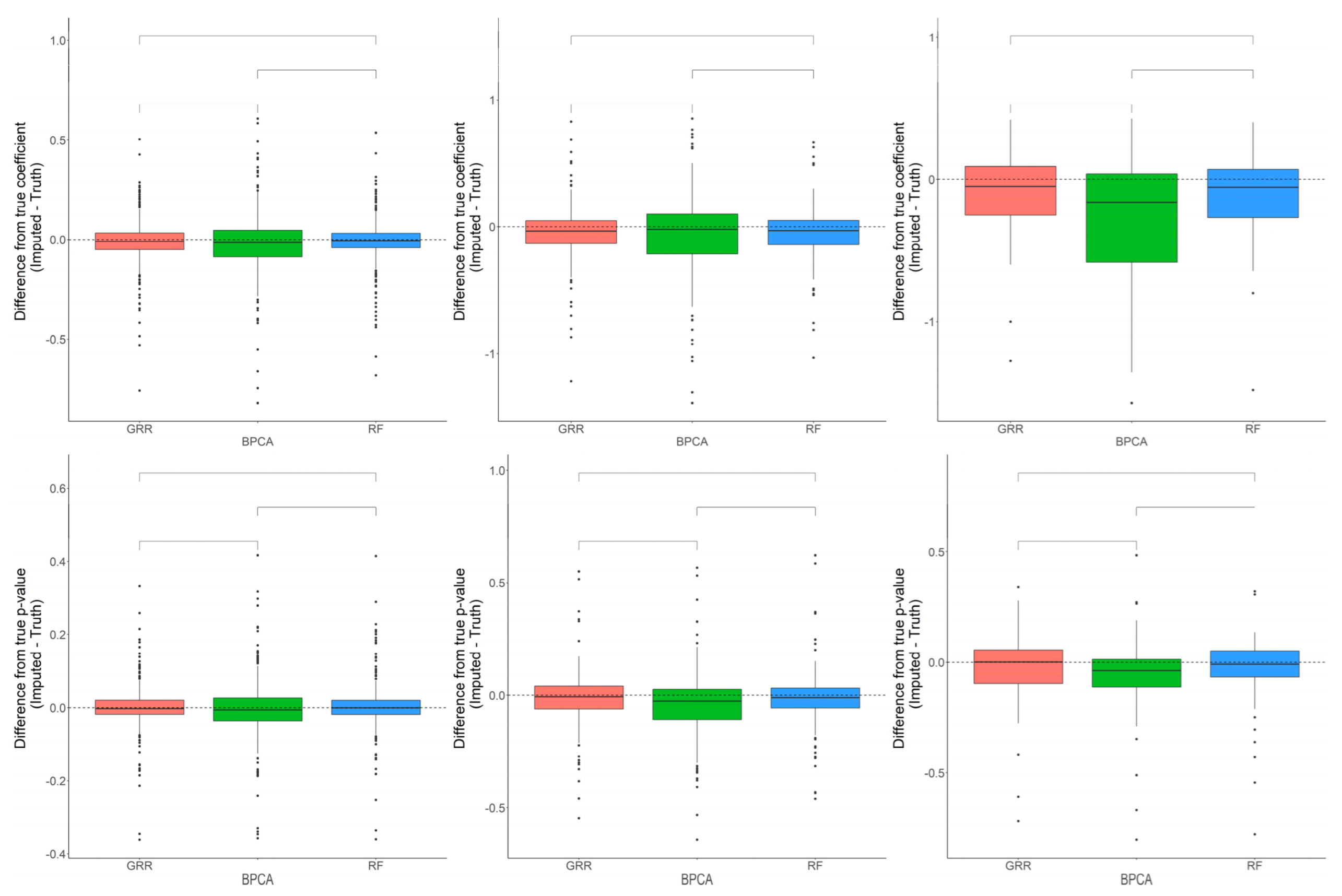
2.2. Evaluation of RF, GRR, and BPCA Imputation Methods on NHP Plasma
2.3. Evaluation of RF, GRR, and BPCA Imputation Methods Using Metabolomics Data from Baboon Liver Biopsy Samples
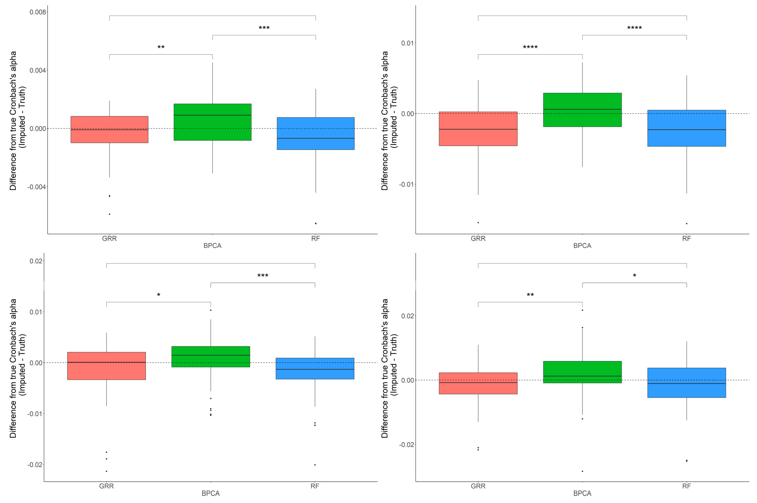
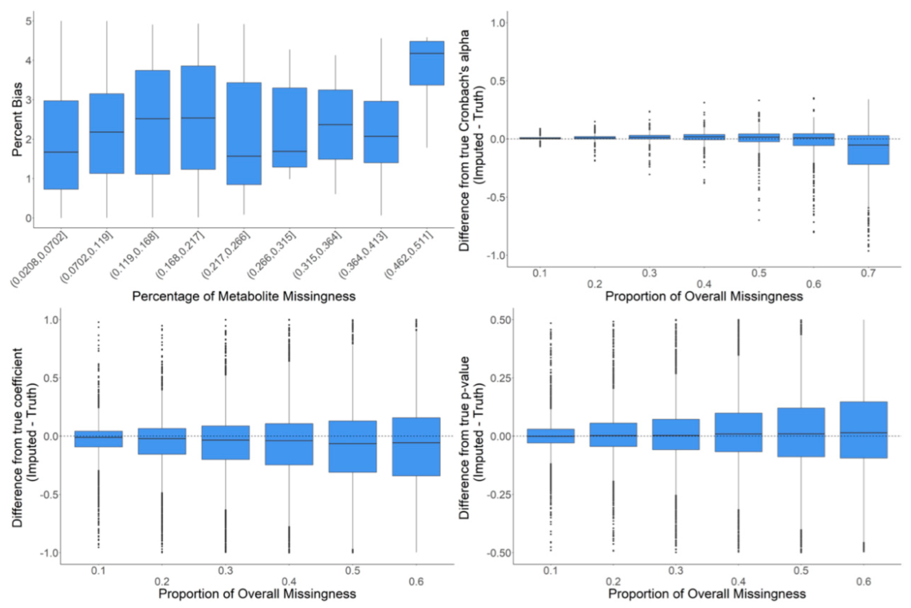
2.4. In-Depth Evaluation of RF Imputation Accuracy at Wide Range of Missingness Using the Entire Baboon Liver HR GC–MS Metabolomics Dataset
3. Discussion
4. Materials and Methods
4.1. Chemicals and Reagents
4.2. Sample Processing
4.3. GC-HR Orbitrap MS Data Acquisition and Preprocessing
4.4. Generation of Missing Values
4.5. Evaluation of Imputation Methods
5. Conclusions
Supplementary Materials
Author Contributions
Funding
Institutional Review Board Statement
Informed Consent Statement
Data Availability Statement
Conflicts of Interest
References
- Faquih, T.; Van Smeden, M.; Luo, J.; Le Cessie, S.; Kastenmüller, G.; Krumsiek, J.; Noordam, R.; Van Heemst, D.; Rosendaal, F.R.; Vlieg, A.V.H.; et al. A Workflow for Missing Values Imputation of Untargeted Metabolomics Data. Metabolites 2020, 10, 486. [Google Scholar] [CrossRef]
- Segers, K.; Declerck, S.; Mangelings, D.; Heyden, Y.V.; Eeckhaut, A.V. Analytical techniques for metabolomic studies: A review. Bioanalysis 2019, 11, 2297–2318. [Google Scholar] [CrossRef]
- Pang, H.; Jia, W.; Hu, Z. Emerging Applications of Metabolomics in Clinical Pharmacology. Clin. Pharmacol. Ther. 2019, 106, 544–556. [Google Scholar] [CrossRef]
- Zhang, A.; Sun, H.; Wang, X. Power of metabolomics in biomarker discovery and mining mechanisms of obesity. Obes. Rev. 2013, 14, 344–349. [Google Scholar] [CrossRef]
- Kohler, I.; Hankemeier, T.; van der Graaf, P.H.; Knibbe, C.A.; van Hasselt, J.C. Integrating clinical metabolomics-based biomarker discovery and clinical pharmacology to enable precision medicine. Eur. J. Pharm. Sci. 2017, 109, S15–S21. [Google Scholar] [CrossRef]
- Dawidowska, J.; Krzyżanowska, M.; Markuszewski, M.J.; Kaliszan, M. The Application of Metabolomics in Forensic Science with Focus on Forensic Toxicology and Time-of-Death Estimation. Metabolites 2021, 11, 801. [Google Scholar] [CrossRef]
- Ardalani, H.; Vidkjær, N.H.; Kryger, P.; Fiehn, O.; Fomsgaard, I.S. Metabolomics unveils the influence of dietary phytochemicals on residual pesticide concentrations in honey bees. Environ. Int. 2021, 152, 106503. [Google Scholar] [CrossRef]
- Wishart, D.S. Metabolomics: Applications to food science and nutrition research. Trends Food Sci. Technol. 2008, 19, 482–493. [Google Scholar] [CrossRef]
- Shah, J.S.; Brock, G.N.; Rai, S.N. Metabolomics data analysis and missing value issues with application to infarcted mouse hearts. BMC Bioinform. 2015, 16, P16. [Google Scholar] [CrossRef]
- Bijlsma, S.; Bobeldijk, I.; Verheij, E.R.; Ramaker, R.; Kochhar, S.; Macdonald, I.A.; van Ommen, B.; Smilde, A.K. Large-scale human metabolomics studies: A strategy for data (pre-) processing and validation. Anal. Chem. 2006, 78, 567–574. [Google Scholar] [CrossRef]
- Hrydziuszko, O.; Viant, M.R. Missing values in mass spectrometry based metabolomics: An undervalued step in the data processing pipeline. Metabolomics 2011, 8, 161–174. [Google Scholar] [CrossRef]
- Wei, R.; Wang, J.; Su, M.; Jia, E.; Chen, S.; Chen, T.; Ni, Y. Missing Value Imputation Approach for Mass Spectrometry-based Metabolomics Data. Sci. Rep. 2018, 8, 663. [Google Scholar] [CrossRef]
- Wei, R.; Wang, J.; Jia, E.; Chen, T.; Ni, Y.; Jia, W. GSimp: A Gibbs sampler based left-censored missing value imputation approach for metabolomics studies. PLoS Comput. Biol. 2018, 14, e1005973. [Google Scholar] [CrossRef]
- Shah, J.S.; Rai, S.N.; DeFilippis, A.P.; Hill, B.G.; Bhatnagar, A.; Brock, G.N. Distribution based nearest neighbor imputation for truncated high dimensional data with applications to pre-clinical and clinical metabolomics studies. BMC Bioinform. 2017, 18, 114. [Google Scholar] [CrossRef]
- Kokla, M.; Virtanen, J.; Kolehmainen, M.; Paananen, J.; Hanhineva, K. Random forest-based imputation outperforms other methods for imputing LC-MS metabolomics data: A comparative study. BMC Bioinform. 2019, 20, 492. [Google Scholar] [CrossRef]
- Ni, Y.; Su, M.; Qiu, Y.; Jia, W.; Du, X. ADAP-GC 3.0: Improved Peak Detection and Deconvolution of Co-eluting Metabolites from GC/TOF-MS Data for Metabolomics Studies. Anal. Chem. 2016, 88, 8802–8811. [Google Scholar] [CrossRef]
- Emmanuel, T.; Maupong, T.; Mpoeleng, D.; Semong, T.; Mphago, B.; Tabona, O. A survey on missing data in machine learning. J. Big Data 2021, 8, 140. [Google Scholar] [CrossRef]
- Zhang, Z. Missing data imputation: Focusing on single imputation. Ann. Transl. Med. 2016, 4, 9. [Google Scholar] [CrossRef]
- Li, H.; Zhao, C.; Shao, F.; Li, G.-Z.; Wang, X. A hybrid imputation approach for microarray missing value estimation. BMC Genom. 2015, 16, S1. [Google Scholar] [CrossRef]
- Taylor, S.L.; Ruhaak, L.R.; Kelly, K.; Weiss, R.H.; Kim, K. Effects of imputation on correlation: Implications for analysis of mass spectrometry data from multiple biological matrices. Brief. Bioinform. 2017, 18, 312–320. [Google Scholar] [CrossRef][Green Version]
- Shah, J.; Brock, G.N.; Gaskins, J. BayesMetab: Treatment of missing values in metabolomic studies using a Bayesian modeling approach. BMC Bioinform. 2019, 20 (Suppl. 24), 673. [Google Scholar] [CrossRef]
- Jin, Z.; Kang, J.; Yu, T. Missing value imputation for LC-MS metabolomics data by incorporating metabolic network and adduct ion relations. Bioinformatics 2018, 34, 1555–1561. [Google Scholar] [CrossRef]
- Kumar, N.; Hoque, A.; Shahjaman; Shahjaman Islam, S.S.; Mollah, N.H. A New Approach of Outlier-robust Missing Value Imputation for Metabolomics Data Analysis. Curr. Bioinform. 2019, 14, 43–52. [Google Scholar] [CrossRef]
- Hong, S.; Lynn, H.S. Accuracy of random-forest-based imputation of missing data in the presence of non-normality, non-linearity, and interaction. BMC Med. Res. Methodol. 2020, 20, 199. [Google Scholar] [CrossRef]
- Gromski, P.S.; Xu, Y.; Kotze, H.L.; Correa, E.; Ellis, D.I.; Armitage, E.G.; Turner, M.L.; Goodacre, R. Influence of missing values substitutes on multivariate analysis of metabolomics data. Metabolites 2014, 4, 433–452. [Google Scholar] [CrossRef]
- Traquete, F.; Luz, J.; Cordeiro, C.; Silva, M.S.; Ferreira, A.E.N. Binary Simplification as an Effective Tool in Metabolomics Data Analysis. Metabolites 2021, 11, 788. [Google Scholar] [CrossRef]
- Rubin, D.B. Multiple Imputation after 18+ Years. J. Am. Stat. Assoc. 1996, 91, 473–489. [Google Scholar] [CrossRef]
- Donders, A.R.T.; van der Heijden, G.J.; Stijnen, T.; Moons, K.G. Review: A gentle introduction to imputation of missing values. J. Clin. Epidemiol. 2006, 59, 1087–1091. [Google Scholar] [CrossRef]
- Van Buuren, S.; Groothuis-Oudshoorn, K. Multivariate Imputation by Chained Equations in R. J. Stat. Softw. 2011, 45, 1–67. [Google Scholar] [CrossRef]
- Misra, B.B.; Olivier, M. High Resolution GC-Orbitrap-MS Metabolomics Using Both Electron Ionization and Chemical Ionization for Analysis of Human Plasma. J. Proteome Res. 2020, 19, 2717–2731. [Google Scholar] [CrossRef]
- Fiehn, O.; Wohlgemuth, G.; Scholz, M.; Kind, T.; Lee, D.Y.; Lu, Y.; Moon, S.; Nikolau, B. Quality control for plant metabolomics: Reporting MSI-compliant studies. Plant J. 2008, 53, 691–704. [Google Scholar] [CrossRef]
- Misra, B.B.; Puppala, S.R.; Comuzzie, A.G.; Mahaney, M.C.; VandeBerg, J.L.; Olivier, M.; Cox, L.A. Analysis of serum changes in response to a high fat high cholesterol diet challenge reveals metabolic biomarkers of atherosclerosis. PLoS ONE 2019, 14, e0214487. [Google Scholar] [CrossRef]
- Tsugawa, H.; Cajka, T.; Kind, T.; Ma, Y.; Higgins, B.; Ikeda, K.; Kanazawa, M.; VanderGheynst, J.; Fiehn, O.; Arita, M. MS-DIAL: Data-independent MS/MS deconvolution for comprehensive metabolome analysis. Nat. Methods 2015, 12, 523–526. [Google Scholar] [CrossRef]
- Lai, Z.; Tsugawa, H.; Wohlgemuth, G.; Mehta, S.; Mueller, M.; Zheng, Y.; Ogiwara, A.; Meissen, J.; Showalter, M.; Takeuchi, K.; et al. Identifying metabolites by integrating metabolome databases with mass spectrometry cheminformatics. Nat. Methods 2018, 15, 53–56. [Google Scholar] [CrossRef]


Publisher’s Note: MDPI stays neutral with regard to jurisdictional claims in published maps and institutional affiliations. |
© 2022 by the authors. Licensee MDPI, Basel, Switzerland. This article is an open access article distributed under the terms and conditions of the Creative Commons Attribution (CC BY) license (https://creativecommons.org/licenses/by/4.0/).
Share and Cite
Ampong, I.; Zimmerman, K.D.; Nathanielsz, P.W.; Cox, L.A.; Olivier, M. Optimization of Imputation Strategies for High-Resolution Gas Chromatography–Mass Spectrometry (HR GC–MS) Metabolomics Data. Metabolites 2022, 12, 429. https://doi.org/10.3390/metabo12050429
Ampong I, Zimmerman KD, Nathanielsz PW, Cox LA, Olivier M. Optimization of Imputation Strategies for High-Resolution Gas Chromatography–Mass Spectrometry (HR GC–MS) Metabolomics Data. Metabolites. 2022; 12(5):429. https://doi.org/10.3390/metabo12050429
Chicago/Turabian StyleAmpong, Isaac, Kip D. Zimmerman, Peter W. Nathanielsz, Laura A. Cox, and Michael Olivier. 2022. "Optimization of Imputation Strategies for High-Resolution Gas Chromatography–Mass Spectrometry (HR GC–MS) Metabolomics Data" Metabolites 12, no. 5: 429. https://doi.org/10.3390/metabo12050429
APA StyleAmpong, I., Zimmerman, K. D., Nathanielsz, P. W., Cox, L. A., & Olivier, M. (2022). Optimization of Imputation Strategies for High-Resolution Gas Chromatography–Mass Spectrometry (HR GC–MS) Metabolomics Data. Metabolites, 12(5), 429. https://doi.org/10.3390/metabo12050429