hcapca: Automated Hierarchical Clustering and Principal Component Analysis of Large Metabolomic Datasets in R


Abstract
1. Introduction
2. Results
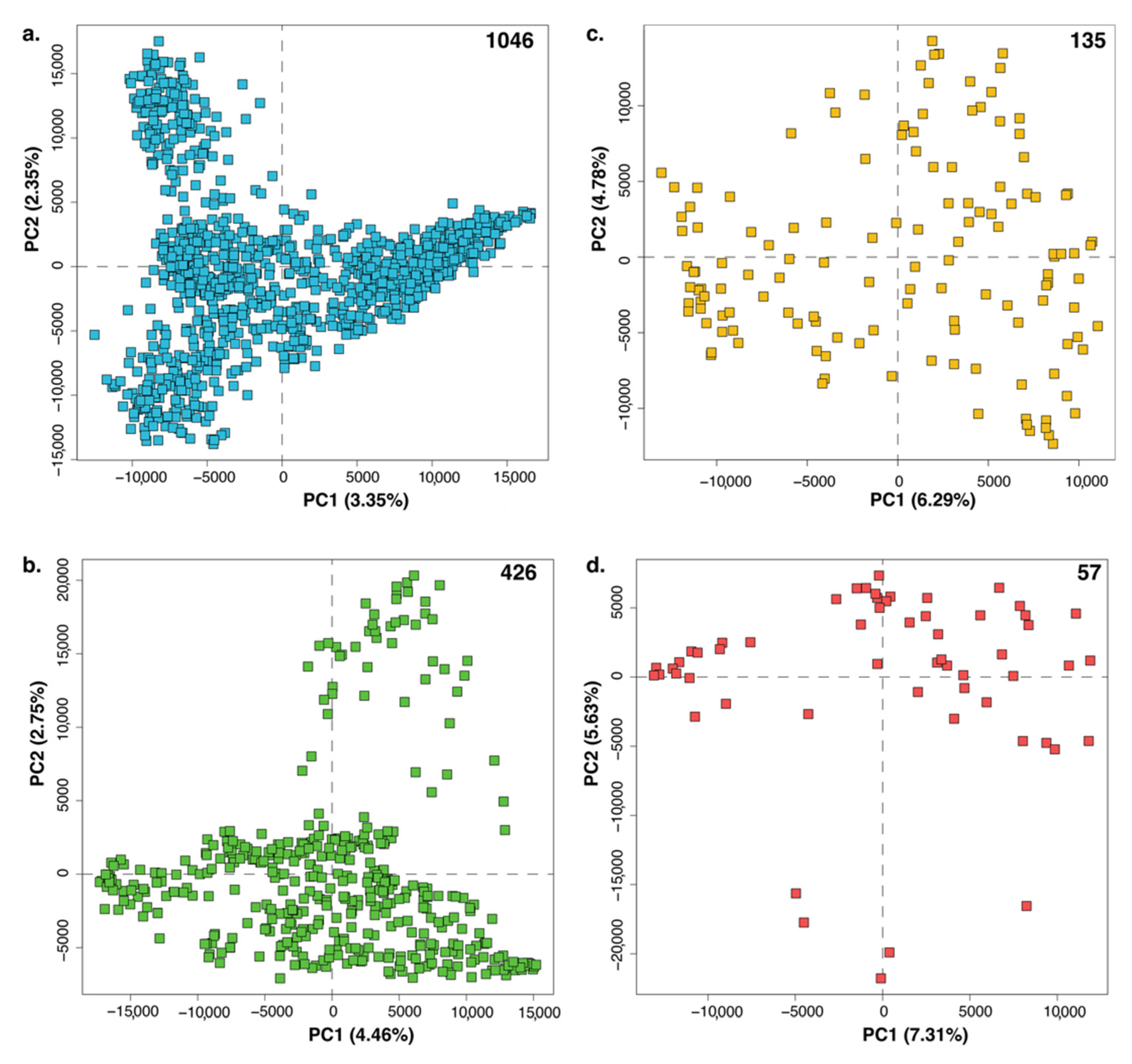
2.1. PCA
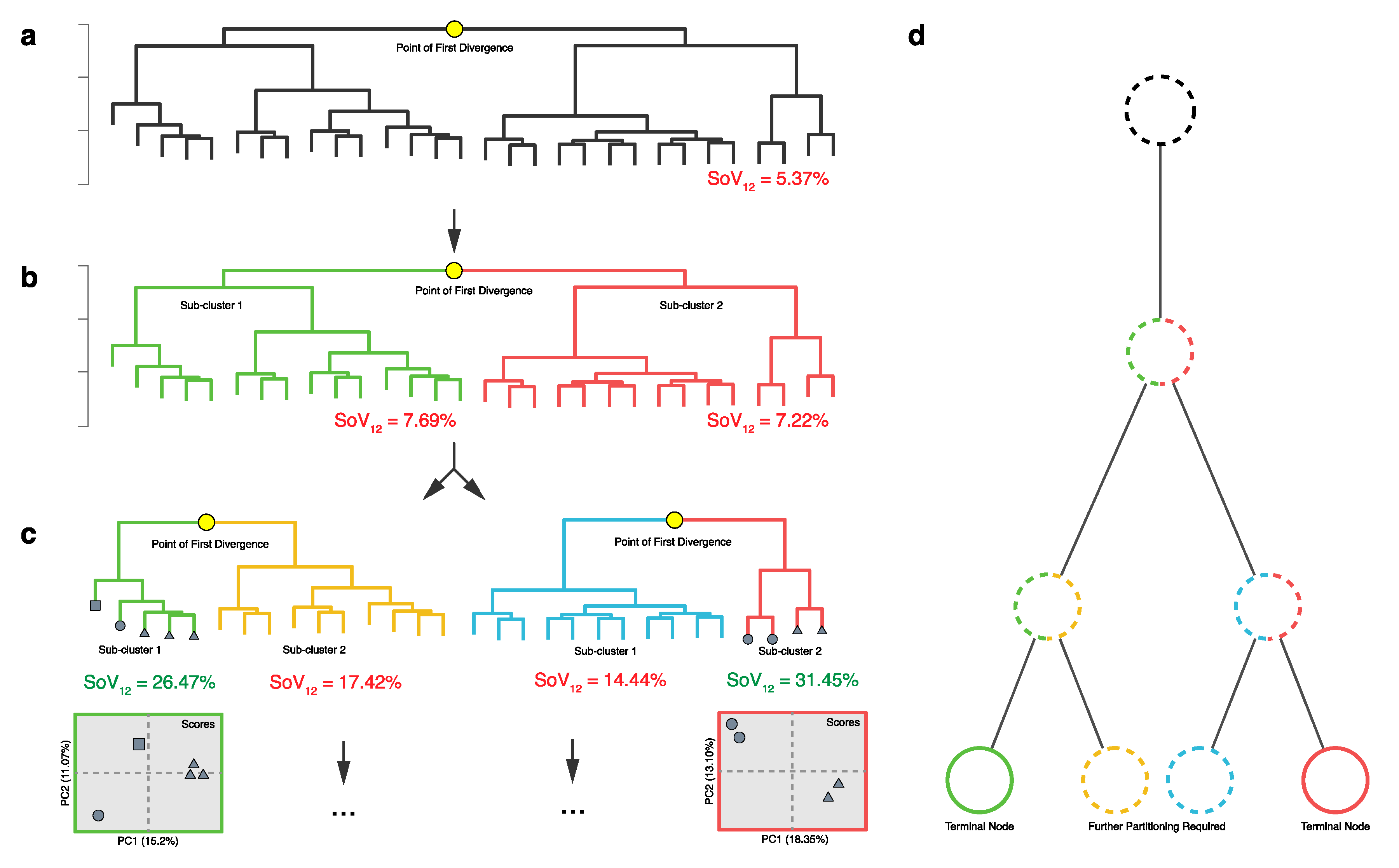
2.2. HCA
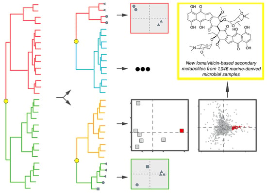
2.3. HCA and PCA in Combination
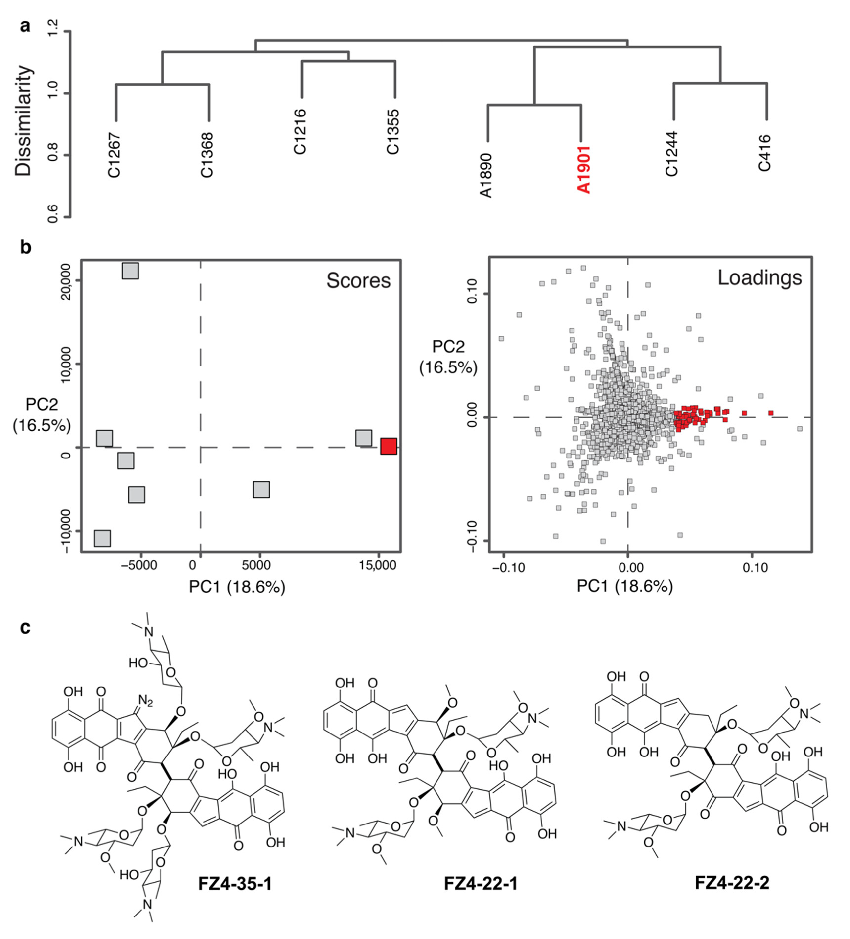
2.4. Identification of Novel Chemistry
3. Materials and Methods
3.1. Generation of Spectral Intensity Tables
3.1.1. Profile Analysis
3.1.2. MZmine2
3.1.3. Data Format
3.1.4. Hierarchical Clustering Analysis (HCA)
3.1.5. Principal Component Analysis (PCA)
3.1.6. Displaying Results
3.1.7. Source Code and Instructions
4. Conclusions
Supplementary Materials
Author Contributions
Funding
Acknowledgments
Conflicts of Interest
References
- Newman, D.J.; Cragg, G.M. Natural products as sources of new drugs over the nearly four decades from 01/1981 to 09/2019. J. Nat. Prod. 2020, 83, 770–803. [Google Scholar] [CrossRef] [PubMed]
- Jensen, P.R.; Moore, B.S.; Fenical, W. The marine actinomycete genus Salinispora: A model organism for secondary metabolite discovery. Nat. Prod. Rep. 2015, 32, 738–751. [Google Scholar] [CrossRef] [PubMed]
- Shen, B. A new golden age of natural products drug discovery. Cell 2015, 163, 1297–1300. [Google Scholar] [CrossRef]
- Harvey, A.L.; Edrada-Ebel, R.; Quinn, R.J. The re-emergence of natural products for drug discovery in the genomics era. Nat. Rev. Drug Discov. 2015, 14, 111–129. [Google Scholar] [CrossRef]
- Koehn, F.E. High impact technologies for natural products screening. Nat. Compd. Drugs Vol. I 2008, 65, 175–210. [Google Scholar] [CrossRef]
- Hou, Y.; Braun, D.R.; Michel, C.R.; Klassen, J.L.; Adnani, N.; Wyche, T.P.; Bugni, T.S. Microbial strain prioritization using metabolomics tools for the discovery of natural products. Anal. Chem. 2012, 84, 4277–4283. [Google Scholar] [CrossRef]
- Chanana, S.; Thomas, C.; Braun, D.; Hou, Y.; Wyche, T.; Bugni, T. Natural product discovery using planes of principal component analysis in R (PoPCAR). Metabolites 2017, 7, 34. [Google Scholar] [CrossRef]
- Clark, C.M.; Costa, M.S.; Sanchez, L.M.; Murphy, B.T. Coupling MALDI-TOF mass spectrometry protein and specialized metabolite analyses to rapidly discriminate bacterial function. Proc. Natl. Acad. Sci. USA 2018, 115, 4981–4986. [Google Scholar] [CrossRef]
- Baker, M. Metabolomics: From small molecules to big ideas. Nat. Methods 2011, 8, 117–121. [Google Scholar] [CrossRef]
- Astarita, G.; Langridge, J. An emerging role for metabolomics in nutrition science. Lifestyle Genom. 2013, 6, 181–200. [Google Scholar] [CrossRef]
- Gibbons, H.; O’Gorman, A.; Brennan, L. Metabolomics as a tool in nutritional research. Curr. Opin. Lipidol. 2015, 26, 30–34. [Google Scholar] [CrossRef] [PubMed]
- Wikoff, W.R.; Anfora, A.T.; Liu, J.; Schultz, P.G.; Lesley, S.A.; Peters, E.C.; Siuzdak, G. Metabolomics analysis reveals large effects of gut microflora on mammalian blood metabolites. Proc. Natl. Acad. Sci. USA 2009, 106, 3698–3703. [Google Scholar] [CrossRef]
- Nicholson, J.K.; Holmes, E.; Kinross, J.; Burcelin, R.; Gibson, G.; Jia, W.; Pettersson, S. Host-gut microbiota metabolic interactions. Science 2012, 336, 1262–1267. [Google Scholar] [CrossRef]
- Demain, A.L.; Fang, A. The natural functions of secondary metabolites. In History of Modern Biotechnology I; Fiechter, A., Ed.; Springer: Berlin/Heidelberg, Germany, 2000; pp. 1–39. ISBN 978-3-540-44964-5. [Google Scholar]
- Newman, D.J.; Cragg, G.M. Endophytic and epiphytic microbes as “sources” of bioactive agents. Front. Chem. 2015, 3, 34. [Google Scholar] [CrossRef]
- Newman, D.J.; Cragg, G.M. Plant endophytes and epiphytes: Burgeoning sources of known and “unknown” cytotoxic and antibiotic agents? Planta Med. 2020. [Google Scholar] [CrossRef] [PubMed]
- Ellis, G.A.; Thomas, C.S.; Chanana, S.; Adnani, N.; Szachowicz, E.; Braun, D.R.; Harper, M.K.; Wyche, T.P.; Bugni, T.S. Brackish habitat dictates cultivable Actinobacterial diversity from marine sponges. PLoS ONE 2017, 12, e0176968. [Google Scholar] [CrossRef]
- Ishihama, Y. Proteomic LC–MS systems using nanoscale liquid chromatography with tandem mass spectrometry. J. Chromatogr. A 2005, 1067, 73–83. [Google Scholar] [CrossRef]
- Thomas, T.; Moitinho-Silva, L.; Lurgi, M.; Björk, J.R.; Easson, C.; Astudillo-García, C.; Olson, J.B.; Erwin, P.M.; López-Legentil, S.; Luter, H.; et al. Diversity, structure and convergent evolution of the global sponge microbiome. Nat. Commun. 2016, 7, 11870. [Google Scholar] [CrossRef]
- Blin, K.; Shaw, S.; Steinke, K.; Villebro, R.; Ziemert, N.; Lee, S.Y.; Medema, M.H.; Weber, T. antiSMASH 5.0: Updates to the secondary metabolite genome mining pipeline. Nucleic Acids Res. 2019, 47, W81–W87. [Google Scholar] [CrossRef]
- Wang, M.; Jarmusch, A.K.; Vargas, F.; Aksenov, A.A.; Gauglitz, J.M.; Weldon, K.; Petras, D.; da Silva, R.; Quinn, R.; Melnik, A.V.; et al. Mass spectrometry searches using MASST. Nat. Biotechnol. 2020, 38, 23–26. [Google Scholar] [CrossRef]
- Nothias, L.F.; Petras, D.; Schmid, R.; Dührkop, K.; Rainer, J.; Sarvepalli, A.; Protsyuk, I.; Ernst, M.; Tsugawa, H.; Fleischauer, M.; et al. Feature-based molecular networking in the GNPS analysis environment. bioRxiv 2019. [Google Scholar] [CrossRef]
- Röst, H.L.; Sachsenberg, T.; Aiche, S.; Bielow, C.; Weisser, H.; Aicheler, F.; Andreotti, S.; Ehrlich, H.-C.; Gutenbrunner, P.; Kenar, E.; et al. OpenMS: A flexible open-source software platform for mass spectrometry data analysis. Nat. Methods 2016, 13, 741–748. [Google Scholar] [CrossRef] [PubMed]
- Tsugawa, H.; Cajka, T.; Kind, T.; Ma, Y.; Higgins, B.; Ikeda, K.; Kanazawa, M.; VanderGheynst, J.; Fiehn, O.; Arita, M. MS-DIAL: Data-independent MS/MS deconvolution for comprehensive metabolome analysis. Nat. Methods 2015, 12, 523–526. [Google Scholar] [CrossRef] [PubMed]
- Lai, Z.; Tsugawa, H.; Wohlgemuth, G.; Mehta, S.; Mueller, M.; Zheng, Y.; Ogiwara, A.; Meissen, J.; Showalter, M.; Takeuchi, K.; et al. Identifying metabolites by integrating metabolome databases with mass spectrometry cheminformatics. Nat. Methods 2018, 15, 53–56. [Google Scholar] [CrossRef]
- Smith, C.A.; Want, E.J.; O’Maille, G.; Abagyan, R.; Siuzdak, G. XCMS: Processing mass spectrometry data for metabolite profiling using Nonlinear Peak Alignment, Matching, and Identification. Anal. Chem. 2006, 78, 779–787. [Google Scholar] [CrossRef]
- Jarmusch, A.K.; Wang, M.; Aceves, C.M.; Advani, R.S.; Aguire, S.; Aksenov, A.A.; Aleti, G.; Aron, A.T.; Bauermeister, A.; Bolleddu, S.; et al. Repository-scale co- and re-analysis of tandem mass spectrometry data. bioRxiv 2019. [Google Scholar] [CrossRef]
- van der Hooft, J.J.J.; Wandy, J.; Young, F.; Padmanabhan, S.; Gerasimidis, K.; Burgess, K.E.V.; Barrett, M.P.; Rogers, S. Unsupervised discovery and comparison of structural families across multiple samples in untargeted metabolomics. Anal. Chem. 2017, 89, 7569–7577. [Google Scholar] [CrossRef]
- Wandy, J.; Zhu, Y.; van der Hooft, J.J.J.; Daly, R.; Barrett, M.P.; Rogers, S. Ms2lda.org: Web-based topic modelling for substructure discovery in mass spectrometry. Bioinformatics 2018, 34, 317–318. [Google Scholar] [CrossRef]
- van der Hooft, J.J.J.; Wandy, J.; Barrett, M.P.; Burgess, K.E.V.; Rogers, S. Topic modeling for untargeted substructure exploration in metabolomics. Proc. Natl. Acad. Sci. USA 2016, 113, 13738–13743. [Google Scholar] [CrossRef]
- Chong, J.; Soufan, O.; Li, C.; Caraus, I.; Li, S.; Bourque, G.; Wishart, D.S.; Xia, J. MetaboAnalyst 4.0: Towards more transparent and integrative metabolomics analysis. Nucleic Acids Res. 2018, 46, W486–W494. [Google Scholar] [CrossRef]
- Pluskal, T.; Castillo, S.; Villar-Briones, A.; Orešič, M. MZmine 2: Modular framework for processing, visualizing, and analyzing mass spectrometry-based molecular profile data. BMC Bioinform. 2010, 11, 395. [Google Scholar] [CrossRef]
- Wang, M.; Carver, J.J.; Phelan, V.V.; Sanchez, L.M.; Garg, N.; Peng, Y.; Nguyen, D.D.; Watrous, J.; Kapono, C.A.; Luzzatto-Knaan, T.; et al. Sharing and community curation of mass spectrometry data with Global Natural Products Social Molecular Networking. Nat. Biotechnol. 2016, 34, 828–837. [Google Scholar] [CrossRef]
- Tripathi, A.; Vazquez-Baeza, Y.; Gauglitz, J.M.; Wang, M.; Duhrkop, K.; Esposito-Nothias, M.; Acharya, D.; Ernst, M.; van der Hooft, J.J.J.; Zhu, Q.; et al. Chemically-informed analyses of metabolomics mass spectrometry data with qemistree. bioRxiv 2020. [Google Scholar] [CrossRef]
- Van Arnam, E.B.; Ruzzini, A.C.; Sit, C.S.; Horn, H.; Pinto-Tomás, A.A.; Currie, C.R.; Clardy, J. Selvamicin, an atypical antifungal polyene from two alternative genomic contexts. Proc. Natl. Acad. Sci. USA 2016, 113, 12940–12945. [Google Scholar] [CrossRef]
- Wyche, T.P.; Piotrowski, J.S.; Hou, Y.; Braun, D.; Deshpande, R.; McIlwain, S.; Ong, I.M.; Myers, C.L.; Guzei, I.A.; Westler, W.M.; et al. Forazoline A: Marine-derived polyketide with antifungal in vivo efficacy. Angew. Chem. Int. Ed. 2014, 53, 11583–11586. [Google Scholar] [CrossRef]
- Abdelmohsen, U.R.; Bayer, K.; Hentschel, U. Diversity, abundance and natural products of marine sponge-associated actinomycetes. Nat. Prod. Rep. 2014, 31, 381–399. [Google Scholar] [CrossRef]
- Abdelmohsen, U.R.; Yang, C.; Horn, H.; Hajjar, D.; Ravasi, T.; Hentschel, U. Actinomycetes from red sea sponges: Sources for chemical and phylogenetic diversity. Mar. Drugs 2014, 12, 2771–2789. [Google Scholar] [CrossRef]
- Yang, Q.; Franco, C.M.M.; Zhang, W. Sponge-associated actinobacterial diversity: Validation of the methods of actinobacterial DNA extraction and optimization of 16S rRNA gene amplification. Appl. Microbiol. Biotechnol. 2015, 99, 8731–8740. [Google Scholar] [CrossRef]
- Edlund, A.; Loesgen, S.; Fenical, W.; Jensen, P.R. Geographic distribution of secondary metabolite genes in the Marine Actinomycete Salinispora arenicola. Appl. Environ. Microbiol. 2011, 77, 5916–5925. [Google Scholar] [CrossRef]
- Nam, S.-J.; Kauffman, C.A.; Jensen, P.R.; Moore, C.E.; Rheingold, A.L.; Fenical, W. Actinobenzoquinoline and Actinophenanthrolines A-C, unprecedented alkaloids from a Marine Actinobacterium. Org. Lett. 2015, 17, 3240–3243. [Google Scholar] [CrossRef]
- Leutou, A.S.; Yang, I.; Kang, H.; Seo, E.K.; Nam, S.-J.; Fenical, W. Nocarimidazoles A and B from a marine-derived Actinomycete of the genus Nocardiopsis. J. Nat. Prod. 2015, 78, 2846–2849. [Google Scholar] [CrossRef] [PubMed]
- Shaaban, K.A.; Saunders, M.A.; Zhang, Y.; Tran, T.; Elshahawi, S.I.; Ponomareva, L.V.; Wang, X.; Zhang, J.; Copley, G.C.; Sunkara, M.; et al. Spoxazomicin D and Oxachelin C, potent Neuroprotective Carboxamides from the Appalachian coal fire-associated isolate Streptomyces sp. RM-14-6. J. Nat. Prod. 2017, 80, 2–11. [Google Scholar] [CrossRef]
- Wang, X.; Zhang, Y.; Ponomareva, L.V.; Qiu, Q.; Woodcock, R.; Elshahawi, S.I.; Chen, X.; Zhou, Z.; Hatcher, B.E.; Hower, J.C.; et al. Mccrearamycins A–D, Geldanamycin-derived Cyclopentenone Macrolactams from an Eastern Kentucky abandoned coal mine microbe. Angew. Chem. Int. Ed. 2017, 56, 2994–2998. [Google Scholar] [CrossRef] [PubMed]
- Wang, X.; Elshahawi, S.I.; Cai, W.; Zhang, Y.; Ponomareva, L.V.; Chen, X.; Copley, G.C.; Hower, J.C.; Zhan, C.-G.; Parkin, S.; et al. Bi- and tetracyclic Spirotetronates from the coal mine fire isolate Streptomyces sp. LC-6-2. J. Nat. Prod. 2017, 80, 1141–1149. [Google Scholar] [CrossRef]
- Derewacz, D.K.; McNees, C.R.; Scalmani, G.; Covington, C.L.; Shanmugam, G.; Marnett, L.J.; Polavarapu, P.L.; Bachmann, B.O. Structure and stereochemical determination of hypogeamicins from a cave-derived actinomycete. J. Nat. Prod. 2014, 77, 1759–1763. [Google Scholar] [CrossRef] [PubMed]
- Beemelmanns, C.; Ramadhar, T.R.; Kim, K.H.; Klassen, J.L.; Cao, S.; Wyche, T.P.; Hou, Y.; Poulsen, M.; Bugni, T.S.; Currie, C.R.; et al. Macrotermycins A-D, glycosylated macrolactams from a termite-associated Amycolatopsis sp. M39. Org. Lett. 2017, 19, 1000–1003. [Google Scholar] [CrossRef]
- Wyche, T.P.; Ruzzini, A.C.; Beemelmanns, C.; Kim, K.H.; Klassen, J.L.; Cao, S.; Poulsen, M.; Bugni, T.S.; Currie, C.R.; Clardy, J. Linear peptides are the major products of a biosynthetic pathway that encodes for cyclic depsipeptides. Org. Lett. 2017, 19, 1772–1775. [Google Scholar] [CrossRef]
- Doroghazi, J.R.; Albright, J.C.; Goering, A.W.; Ju, K.; Haines, R.R.; Tchalukov, K.A.; Labeda, D.P.; Kelleher, N.L.; Metcalf, W.W. A roadmap for natural product discovery based on large-scale genomics and metabolomics. Nat. Chem. Biol. 2014, 10, 963–968. [Google Scholar] [CrossRef]
- Ziemert, N.; Lechner, A.; Wietz, M.; Millan-Aguinaga, N.; Chavarria, K.L.; Jensen, P.R. Diversity and evolution of secondary metabolism in the marine actinomycete genus Salinispora. Proc. Natl. Acad. Sci. USA 2014, 111, E1130–E1139. [Google Scholar] [CrossRef] [PubMed]
- Goodwin, C.R.; Sherrod, S.D.; Marasco, C.C.; Bachmann, B.O.; Schramm-Sapyta, N.; Wikswo, J.P.; McLean, J.A. Phenotypic mapping of metabolic profiles using self-organizing maps of high-dimensional mass spectrometry data. Anal. Chem. 2014, 86, 6563–6571. [Google Scholar] [CrossRef]
- Goodwin, C.R.; Covington, B.C.; Derewacz, D.K.; McNees, C.R.; Wikswo, J.P.; McLean, J.A.; Bachmann, B.O. Structuring microbial metabolic responses to multiplexed stimuli via self-organizing metabolomics Maps. Chem. Biol. 2015, 22, 661–670. [Google Scholar] [CrossRef] [PubMed]
- Altman, N.; Krzywinski, M. Points of significance: Clustering. Nat. Methods 2017, 14, 545–546. [Google Scholar] [CrossRef]
- Frank, A.M.; Bandeira, N.; Shen, Z.; Tanner, S.; Briggs, S.P.; Smith, R.D.; Pevzner, P.A. Clustering millions of tandem mass spectra. J. Proteome Res. 2008, 7, 113–122. [Google Scholar] [CrossRef]
- Meinicke, P.; Lingner, T.; Kaever, A.; Feussner, K.; Göbel, C.; Feussner, I.; Karlovsky, P.; Morgenstern, B. Metabolite-based clustering and visualization of mass spectrometry data using one-dimensional self-organizing maps. Algorithms Mol. Biol. 2008, 3, 9. [Google Scholar] [CrossRef] [PubMed]
- Broeckling, C.D.; Afsar, F.A.; Neumann, S.; Ben-Hur, A.; Prenni, J.E. RAMClust: A novel feature clustering method enables spectral-matching-based annotation for metabolomics data. Anal. Chem. 2014, 86, 6812–6817. [Google Scholar] [CrossRef]
- Damian, D.; Orešič, M.; Verheij, E.; Meulman, J.; Friedman, J.; Adourian, A.; Morel, N.; Smilde, A.; van der Greef, J. Applications of a new subspace clustering algorithm (COSA) in medical systems biology. Metabolomics 2007, 3, 69–77. [Google Scholar] [CrossRef]
- Li, X.; Lu, X.; Tian, J.; Gao, P.; Kong, H.; Xu, G. Application of fuzzy c-means clustering in data analysis of metabolomics. Anal. Chem. 2009, 81, 4468–4475. [Google Scholar] [CrossRef]
- Depke, T.; Franke, R.; Brönstrup, M. Clustering of MS2 spectra using unsupervised methods to aid the identification of secondary metabolites from Pseudomonas aeruginosa. J. Chromatogr. B 2017, 1071, 19–28. [Google Scholar] [CrossRef]
- Clark, C.M.; Costa, M.S.; Conley, E.; Li, E.; Sanchez, L.M.; Murphy, B.T. Using the open-source MALDI TOF-MS IDBac pipeline for analysis of microbial protein and specialized metabolite data. J. Vis. Exp. 2019, 147, e59219. [Google Scholar] [CrossRef]
- Krug, D.; Zurek, G.; Revermann, O.; Vos, M.; Velicer, G.J.; Müller, R. Discovering the hidden secondary metabolome of Myxococcus xanthus: A study of intraspecific diversity. Appl. Environ. Microbiol. 2008, 74, 3058–3068. [Google Scholar] [CrossRef] [PubMed]
- Krug, D.; Zurek, G.; Schneider, B.; Garcia, R.; Müller, R. Efficient mining of myxobacterial metabolite profiles enabled by liquid chromatography-electrospray ionisation-time-of-flight mass spectrometry and compound-based principal component analysis. Anal. Chim. Acta 2008, 624, 97–106. [Google Scholar] [CrossRef]
- Robertson, V.; Haltli, B.; McCauley, E.; Overy, D.; Kerr, R. Highly variable bacterial communities associated with the Octocoral Antillogorgia elisabethae. Microorganisms 2016, 4, 23. [Google Scholar] [CrossRef]
- Forner, D.; Berrué, F.; Correa, H.; Duncan, K.; Kerr, R.G. Chemical dereplication of marine actinomycetes by liquid chromatography-high resolution mass spectrometry profiling and statistical analysis. Anal. Chim. Acta 2013, 805, 70–79. [Google Scholar] [CrossRef] [PubMed]
- Covington, B.C.; McLean, J.A.; Bachmann, B.O. Comparative mass spectrometry-based metabolomics strategies for the investigation of microbial secondary metabolites. Nat. Prod. Rep. 2017, 34, 6–24. [Google Scholar] [CrossRef] [PubMed]
- Derewacz, D.K.; Covington, B.C.; McLean, J.A.; Bachmann, B.O. Mapping microbial response metabolomes for induced natural product discovery. ACS Chem. Biol. 2015, 10, 1998–2006. [Google Scholar] [CrossRef] [PubMed]
- Betancur, L.A.; Naranjo-Gaybor, S.J.; Vinchira-Villarraga, D.M.; Moreno-Sarmiento, N.C.; Maldonado, L.A.; Suarez-Moreno, Z.R.; Acosta-González, A.; Padilla-Gonzalez, G.F.; Puyana, M.; Castellanos, L.; et al. Marine Actinobacteria as a source of compounds for phytopathogen control: An integrative metabolic-profiling/bioactivity and taxonomical approach. PLoS ONE 2017, 12, e0170148. [Google Scholar] [CrossRef] [PubMed]
- He, H.; Ding, W.-D.; Bernan, V.S.; Richardson, A.D.; Ireland, C.M.; Greenstein, M.; Ellestad, G.A.; Carter, G.T. Lomaiviticins A and B, potent antitumor antibiotics from Micromonospora lomaivitiensis. J. Am. Chem. Soc. 2001, 123, 5362–5363. [Google Scholar] [CrossRef]
- Woo, C.M.; Beizer, N.E.; Janso, J.E.; Herzon, S.B. Isolation of Lomaiviticins C–E, transformation of Lomaiviticin C to Lomaiviticin A, complete structure elucidation of Lomaiviticin A, and structure–activity analyses. J. Am. Chem. Soc. 2012, 134, 15285–15288. [Google Scholar] [CrossRef]
- Lever, J.; Krzywinski, M.; Altman, N. Points of significance: Principal component analysis. Nat. Methods 2017, 14, 641–642. [Google Scholar] [CrossRef]
- Ringnér, M. What is principal component analysis? Nat. Biotechnol. 2008, 26, 303–304. [Google Scholar] [CrossRef]
- Macintyre, L.; Zhang, T.; Viegelmann, C.; Martinez, I.J.; Cheng, C.; Dowdells, C.; Abdelmohsen, U.R.; Gernert, C.; Hentschel, U.; Edrada-Ebel, R. Metabolomic tools for secondary metabolite discovery from Marine Microbial Symbionts. Mar. Drugs 2014, 12, 3416–3448. [Google Scholar] [CrossRef] [PubMed]
- Carr, G.; Poulsen, M.; Klassen, J.L.; Hou, Y.; Wyche, T.P.; Bugni, T.S.; Currie, C.R.; Clardy, J. Microtermolides A and B from termite-associated Streptomyces sp. and structural revision of vinylamycin. Org. Lett. 2012, 14, 2822–2825. [Google Scholar] [CrossRef] [PubMed]
- Hou, Y.; Tianero, M.D.B.; Kwan, J.C.; Wyche, T.P.; Michel, C.R.; Ellis, G.A.; Vazquez-Rivera, E.; Braun, D.R.; Rose, W.E.; Schmidt, E.W.; et al. Structure and biosynthesis of the antibiotic bottromycin D. Org. Lett. 2012, 14, 5050–5053. [Google Scholar] [CrossRef] [PubMed]
- Reich, D.; Price, A.L.; Patterson, N. Principal component analysis of genetic data. Nat. Genet. 2008, 40, 491–492. [Google Scholar] [CrossRef]
- Chang, W.; Cheng, J.; Allaire, J.J.; Xie, Y.; McPherson, J. Shiny: Web Application Framework for R. 2020. Available online: https://cran.r-project.org/web/packages/shiny/index.html (accessed on 18 June 2020).
- Chang, W.; Ribeiro, B.B. Shinydashboard: Create Dashboards with “Shiny”. 2018. Available online: https://cran.r-project.org/web/packages/shinydashboard/index.html (accessed on 18 June 2020).
- R Core Team. R: A Language and Environment for Statistical Computing; R Foundation for Statistical Computing: Vienna, Austria, 2018. [Google Scholar]
- van den Berg, R.A.; Hoefsloot, H.C.J.; Westerhuis, J.A.; Smilde, A.K.; van der Werf, M.J. Centering, scaling, and transformations: Improving the biological information content of metabolomics data. BMC Genom. 2006, 7, 142. [Google Scholar] [CrossRef]


© 2020 by the authors. Licensee MDPI, Basel, Switzerland. This article is an open access article distributed under the terms and conditions of the Creative Commons Attribution (CC BY) license (http://creativecommons.org/licenses/by/4.0/).
Share and Cite
Chanana, S.; Thomas, C.S.; Zhang, F.; Rajski, S.R.; Bugni, T.S. hcapca: Automated Hierarchical Clustering and Principal Component Analysis of Large Metabolomic Datasets in R. Metabolites 2020, 10, 297. https://doi.org/10.3390/metabo10070297
Chanana S, Thomas CS, Zhang F, Rajski SR, Bugni TS. hcapca: Automated Hierarchical Clustering and Principal Component Analysis of Large Metabolomic Datasets in R. Metabolites. 2020; 10(7):297. https://doi.org/10.3390/metabo10070297
Chicago/Turabian StyleChanana, Shaurya, Chris S. Thomas, Fan Zhang, Scott R. Rajski, and Tim S. Bugni. 2020. "hcapca: Automated Hierarchical Clustering and Principal Component Analysis of Large Metabolomic Datasets in R" Metabolites 10, no. 7: 297. https://doi.org/10.3390/metabo10070297
APA StyleChanana, S., Thomas, C. S., Zhang, F., Rajski, S. R., & Bugni, T. S. (2020). hcapca: Automated Hierarchical Clustering and Principal Component Analysis of Large Metabolomic Datasets in R. Metabolites, 10(7), 297. https://doi.org/10.3390/metabo10070297