The EU’s Gain (Loss) from More Emission Trading Flexibility—A CGE Analysis with Parallel Emission Trading Systems

Abstract

The EU has established the world’s first cross-border emission-trading systems (ETS) for greenhouse gas (GHG) emissions, currently covering aviation, emission-intensive sectors, and electricity (EITE). The EU Commission has offered to apply emissions trading in new sectors where emissions from maritime transport will be incorporated into the current EU ETS, while a separated emissions trading system will cover emissions from road transport and the building sector. This paper employs a multi-regional multi-sectoral computable general equilibrium (CGE) model with two simultaneous international emission permit markets. After examining the abatement costs for the EU regions, various policy scenarios are implemented to study the welfare effects of forming an ETS covering the sectors other than EITE (NEIT) and its linking with the EITE sectors under two different baselines and four emission reduction targets. The results provide several important insights: (i) Marginal abatement costs in Germany and the Eastern European Union region (EEU) are significantly lower than in the rest of the EU regions. (ii) The carbon price in the emission permit market covering NEIT is significantly higher than the carbon price in the emission permit market covering EITE. (iii) Germany and EEU appear as notable suppliers of emission permits in both markets. (iv) There is a significant aggregate welfare gain under the scenario in which the ETS covering NEIT co-exists parallel with the ETS covering EITE. (v) The aggregate welfare in the EU under the full integration of EITE and NEIT may fall below its value under the scenario with two parallel emission permit markets.

1. Introduction

Urgent response against climate change caused by anthropogenic greenhouse gas emissions is essential to counteract global risks, including food production shortages, rising sea levels, and catastrophic flooding. In this regard, emission abatement is the most viable option, which requires international efforts and cooperation. International top–down policy approaches, such as the Kyoto approach, have been assumed to be unsuccessful, and hence, bottom–up policy approaches, such as the Paris approach, have gained more attention [1]. At the 21st Conference of the Parties in Paris in 2015, member states to the United Nations Framework Convention on Climate Change (UNFCCC) agreed to develop a sustainable low-carbon pathway via the stimulation of actions and enhancing low-carbon investments [2]. The Paris Agreement aims to keep the increase in global average temperature to well below 2 °C above pre-industrial level and pursue endeavors to limit the increase to 1.5 °C [2]. Most individual countries, including European countries, submitted national pledges of specific cuts in their carbon emissions by 2030, so-called Nationally Determined Contributions (NDCs). Note that there are countries that stated their emission reductions for other years, such as 2025 or 2035, and some countries did not even provide any quantified commitments and only provided qualitative efforts [3].

These NDCs can be met through different market-based instruments such as the carbon pricing and emission trading system (ETS) (also known as “cap and trade”). By internalizing the costs of climate damage into prices, ETS allows for the international trade mechanism being taken into account and regions forming coalitions. Studies show that the linking of ETS can increase the efficiency of international greenhouse gas mitigation [4,5,6,7,8]. For this reason, the linking of ETS is described as a central policy instrument to the Paris Agreement [9] or viewed as a contingency option for achieving the Paris targets [1].

Nevertheless, it is possible that the linking of ETS results in welfare losses in some of participating regions, and the aggregate welfare of the participating regions declines for reasons including international trade (also known as terms-of-trade) effects [7,10,11]. As an example mechanism for this, compared to a non-trading scenario, if a specific region regains its international competitiveness through its relatively lower carbon prices while the rest of the participating regions become relatively less competitive through relatively higher carbon prices in an emission-trading scenario, then the region may gain welfare. At the same time, the rest of the regions may lose welfare. On this subject, some studies show that even if a region does not implement any climate policy, its welfare may be affected by the climate policy in other regions via terms-of-trade (ToT) effects [11,12]. Peterson and Weitzel [13] suggest that in a global ETS, transfer payments are essential to balance indirect market effects. In this article, for the sake of brevity, transfer payments are not implemented. Studies such as [14,15,16] discuss whether the different policy scenarios are stable or self-enforcing. If coalitions are not stable or self-enforcing, redistribution schemes are required to make them so.

The EU has one of the world’s most ambitious abatement policies and has established the world’s first cross-border carbon market and the largest by emissions covered at the time of establishment. The EU 2030 Climate and Energy Framework documents abatement intentions for sectors covered by the EU emission trading system (EU ETS) [17]. Several papers have analyzed the welfare and distributional effects of the EU ETS (e.g., Tol [18]; Böhringer [19]; Vielle [20]). In a multi-regional multi-sectoral CGE model intercomparison study using the GTAP9 data set [21], the 36th round of Energy Modeling Forum (EMF36) investigates various policy regimes to fulfill different ambition levels and the widespread economic impacts such regimes may bring about [6]. The Core EMF36 demonstrates that the results on the EU notably depend on the model in hand [6]. While the Core EMF36 reports on the EU as an aggregate region, there are individual contributions that consider further disaggregating the EU [22,23,24]. Analyzing the impacts of Norway joining the EU ETS, Faehn and Yonezawa [22] model scenarios where two emission trading systems, with one international price each, co-exist. Their focus is on Norway, a small-open economy, while the rest of the EU is aggregated into one region. Disaggregating the EU into eight regions, Winkler et al. [24] look into the circumstances under which ETS linking between the EU and China is most beneficial to the EU or China, but they do not consider two concurrent emission trading systems. Moreover, Kriegler et al. [25] states that the EU reliance on coal and natural gas imports can decline more rapidly than oil imports—oil imports pose itself as a bottleneck, where the inefficiencies due to oil phase-out can create more elevated production costs.

The EU Commission has proposed applying emissions trading in new sectors where more acute mitigations are required to reach the 2030 target. According to the proposition, emissions from maritime transport will be incorporated into the current EU ETS, while a separate emissions trading system will cover emissions from fuels utilized in road transport and the building sector [26]. Therefore, it is worthwhile to analyze the implications of such a proposal and its distributional impacts on the region.

In this study, the multi-regional multi-sectoral CGE model by Khabbazan and von Hirschhausen [11] is used and the option that two international emission permit markets can be formed simultaneously is added. The underlying CGE model that Khabbazan and von Hirschhausen [11] is based upon has also been used for the model intercomparison studies in Böhringer et al. [6] and Akın-Olçum et al. [4]. Using the GTAP10 Power data set [27,28], the EU region is further disaggregated into nine regions. The regional disaggregation of the EU is similar to that of Winkler et al. [24], except that Ireland is disaggregated from Great Britain—since 2021, the UK has not been part of the EU ETS anymore. Then, after forward-calibration of the model based on International Energy Outlook (IEO) [29] and World Energy Outlook (WEO) [30] projections until 2030, marginal abatement cost curves (MACCs) are derived. In addition to the REF scenario in which no region collaborates, three policy scenarios are simulated:

 EU_EITE 

where an ETS covers the emission-intensive sectors and electricity (EITE), mimicking the current EU ETS sectors, is formed.

 EU_MIX 

where, in addition to an ETS covering EITE, another ETS covers NEIT sectors (i.e., all sectors rather than EITE).

 EU_Full 

where one ETS covers all sectors.

Each policy scenario is run for four emission reduction targets, i.e., NDC, conditional NDC (NDC+), NDC to meet the 2-degree global average temperature target (NDC-2C), and NDC to meet the 1.5-degree global average temperature target (NDC-1.5C). Note that only the NDC targets are politically approved documents [3], and the rest (NDC+, NDC-2C, and NDC-1.5C) are hypothetically calculated. Please see Section 2.3.

Therefore, there are four main research questions:

• What are the cost-effectiveness and welfare impacts of current the EU ETS, i.e., moving from the REF scenario to EU_EITE?
• What does the EU region gain in effectiveness terms from involving in further regional flexibility, i.e., moving from EU_EITE to EU_MIX, and what are the distributional implications?
• How will a fully flexible EU ETS regime impact effectiveness and welfare in the EU regions, i.e., moving to EU_Full?
• How will the impacts evolve under different baselines and ambition levels?

Previous articles have studied linking regional allowance trading systems [10,22,31,32,33,34,35]. Economic theories suggest that the abatement cost for the coalition as a whole “unambiguously declines as more flexibility is introduced” [22]. In this regard, the overall reduction in the abatement cost is not necessarily associated with an overall increase in total welfare. Likewise, a Pareto improvement is not necessarily reached—some members of the coalition might lose [32,34].

The paper’s results on marginal abatement costs (MACs) indicate that NEIT MACs are more expensive than EITE MACs under both baselines. In addition, East Europe (EEU) and Germany have the lowest MACs among the EU regions. Additionally, the MACs under the WEO baseline are slightly higher than under the IEO baseline. In addition, this paper’s results suggest that the common carbon price in the emission permit market covering the NEIT is significantly higher than the common carbon price in the emission permit market covering the EITE. Moreover, moving from the EU_EITE scenario to the EU_MIX scenario can decrease the abatement cost for the EU and bring about a significant welfare gain as a whole. In addition, the results suggest that moving from the EU_MIX to the EU_Full scenario may decrease the overall welfare. The underlying reason is the slight loss of international competitiveness under the EU_Full scenario.

This paper proceeds as follows: the following section describes the framework for this paper in detail. Section 3 presents and interprets the modeling results. Section 4 comprises a discussion, and Section 5 concludes the paper.

2. Framework

This section explains the theoretical and numerical framework in this paper. It details the model and data, regional and sectoral aggregation, calibration of baselines, procedure to generate marginal abatement costs curves (MACCs), and policy scenarios (cooperation options).

2.1. Model and Data

This paper’s analysis is performed with the standard multi-regional, multi-sectoral, static computable-general equilibrium CGE-MOD [11]. CGE-MOD is a global trade and energy model with four power generation technologies (renewables, nuclear, fossil, and others). The core code is based on the GTAPinGAMS model type by Lanz and Rutherford [36], and it is extended based on the model developed by Böhringer and Rutherford [37] to incorporate carbon pricing and ETS. Figure 1 and Figure 2 show the nesting structure for non-fossil fuel production and fossil fuel production, respectively. The fossil-fuel production (extractions) technology includes a specific immobile factor to calibrate local supply responses and natural resources income. The international commodity markets are competitive, where imports are represented following the Armington approach [38]. In addition, constant-elasticity-of-transformation (CET) functions are applied to determine imperfect substitutions between exports and supplies of domestic goods.

The reference data (quantities, prices, and exogenous elasticities) specify the free parameters of the model’s functional forms. In this paper, the reference data are based on the GTAP 10 Power database with detailed accounts of regional production, consumption, bilateral trade flows, energy uses, and CO₂ emissions for the year 2014 [27,28]. The main elasticity values, such as elasticities between energy inputs and non-energy inputs, elasticities between production factors (labor, capital, and resources), the elasticities in international trade (so-called Armington elasticities), and the supply elasticities of fossil fuels (coal, gas, and oil), are presented in

Table 1. Main elasticity values.

Item	Value
Elasticity of supply of fossil fuels	Beckman et al. [41]
Elasticity of substitution on top of technology nest in fossil production $\left({\sigma }_{\mathrm{fos},\mathrm{r}}^s\right)$	Beckman et al. [41]
Armington elasticities for gas and oil	Böhringer and Rutherford [37] *
CET elasticities for gas and oil	Böhringer and Rutherford [37] *
Other CET and Armington elasticities	GTAP *; Lanz and Rutherford [36] *
Elasticity of substitution between factors $\left({\sigma }_{\mathrm{g},\mathrm{r}}^{KL}\right)$	Okagawa and Ban [42]
Elasticity of substitution between composite factors and energy $\left({\sigma }_{\mathrm{g},\mathrm{r}}^{KLE}\right)$	Okagawa and Ban [42]
Elasticity of substitution between power technologies $\left({\sigma }_{\mathrm{g},\mathrm{r}}^{ele}\right)$	Khabbazan and von Hirschhausen [11] *
Elasticity of substitution between non electricity energy $\left({\sigma }_{\mathrm{g},\mathrm{r}}^{nele}\right)$	Böhringer and Rutherford [37]
Elasticity of substitution between non electricity and electricity $\left({\sigma }_{\mathrm{g},\mathrm{r}}^e\right)$	Böhringer and Rutherford [37]
Elasticity of substitution between intermediate inputs $\left({\sigma }_{\mathrm{g},\mathrm{r}}^M\right)$	Okagawa and Ban [42]
Elasticity of substitution between KLE and intermediate inputs $\left({\sigma }_{\mathrm{g},\mathrm{r}}^{KLEM}\right)$	Okagawa and Ban [42]

* Elasticities that are 50% increased in 2030 compared to their values in the benchmark.

. CGE models are generally sensitive to critical assumptions such as the elasticity levels in the nesting structure. Therefore, it is crucial to see how key results are sensitive to the current assumptions. Khabbazan and von Hirschhausen [11] tested the sensitivity of their results to Armington elasticities and the elasticity of substitution in electricity composite, and they showed that the welfare results are not significantly affected under all sensitivity analyses scenarios. As the same model is applied here, the sensitivity analysis is skipped for the sake of brevity. All simulations have been performed in General Algebraic Modeling System (GAMS) software [39] and are solved by employing the solver PATH [40].

2.2. Regions and Sectors

For the sake of result tractability and numerical efficiency, the regional disaggregation of the EU in this paper is built on those used in Winkler et al. [24] (see

Table 2. Model regions and sectors.

Countries and Regions	Sectors and Commodities
European Regions	Non-Electric Energy
DEU (Germany)	COL (Coal)
FRA (France)	CRU (Crude oil)
BLX (Belgium, Luxembourg, The Netherlands)	GAS (Natural gas)
EEU (Bulgaria, Croatia, Czech Republic, Hungary,	OIL (Petroleum and refined oil products)
Poland, Romania, Slovakia, Slovenia, the Baltic States)	Electric Energy
ILI (Ireland, Iceland, Liechtenstein)	EFF * (Fossil-fuel-based electricity)
SCA (Denmark, Finland, Norway, Sweden)	ENB * (Nuclear-based electricity)
SEU (Austria, Cyprus, Greece, Italy, Malta, Portugal, Spain)	ERN * (Renewable-based electricity including hydro, solar,
GBR (United Kingdom)	and wind)
REU (Rest of Europe (non-ETS): Switzerland,	EOT * (Other electricity including geothermal and biofuels)
Albania, Belarus, Ukraine, Serbia, Rest of EFTA)	TND * (Transmission and distribution of electricity)
Other Regions	Non-Energy
CHN (China)	AGR (Agriculture)
JPN (Japan)	ATP * (Aviation)
KOR (South Korea)	EIT * (Energy-intensive trade-exposed)
AFR (Africa)	MFR (Other manufacturing)
ANZ (Australia and New Zealand)	SER (Services)
BRA (Brazil)	TRN (Other transports)
CAN (Canada)	Final Demand
IND (India)	RA (Representative agent; household)
MEA (The Middle East)	GOV (Government)
OAM (Other Americas)	INV (Investment)
OAS (Other Asia)
RUS (Russia)
USA (The United States)

* Sectors included in EITE in this paper.

), except that Ireland is disaggregated from Great Britain and is aggregated with Iceland and Liechtenstein, collectively forming ILI. Therefore, the EU is disaggregated into nine regions: Germany; France; BLX (including Belgium, Luxembourg, and The Netherlands); EEU (east European countries); ILI (including Ireland, Iceland, and Liechtenstein); SCA (Scandinavian countries); SEU (south European countries); GBR (Great Britain); REU (the rest of Europe which do not participate in the current EU ETS). Hence, there are 22 model regions. The remaining 13 regions align with the EMF36 harmonization [6]. The current EU ETS omits GBR and REU, and hence, in this paper, only the results for seven European regions are reported. These regions are marked bold in Table 2. Hereafter, EUR refers to Europe, as a whole, excluding GBR and REU.

The sectoral disaggregations align with the EMF36 harmonization [6], except that aviation transportation (ATP) is disaggregated from the other transportation means (TRN). Therefore, there are 18 sectors in the model, including three final demands (representative agent, government, and investment) (see Table 2). Following Khabbazan and von Hirschhausen [11], the electricity sector is disaggregated into four different technologies: renewables (comprising hydro, solar, and wind technologies), nuclear, fossil, and others (including geothermal and bio-fuel technologies). The remaining sectors also align with the EMF36 harmonization [6], except that aviation is disaggregated from the other transporation means. Therefore, there are six production sectors (agriculture, aviation, energy-intensive trade-exposed goods, other transports, other manufacturing, and services) and four energy sectors (crude oil, refined oil products, coal, gas). In Table 2, the sectors currently covered by EU ETS (EITE) are marked with a superscripted asterisk. The rest of the sectors are NEIT sectors.

As a comparison of the selected regions in the benchmark,

Table 3. CO₂ emission, GDP, emission intensity, and percentage of emission by EITE and NEIT sectors for the selected model regions in the benchmark in 2014.

Region	Emission	GDP	Emission Intensity	Emission (%)
	MtCO2	B$	MtCO2/B$	EITE	NEIT
DEU	678.2	3864.2	0.18	59.3	40.7
FRA	318.2	2843.2	0.11	28.2	71.8
BLX	283.0	1472.9	0.19	44.7	55.3
EEU	584.4	1464.4	0.40	54.6	45.4
ILI	48.4	273.4	0.18	49.8	50.2
SCA	205.7	1697.6	0.12	34.2	65.8
SEU	830.2	4455.4	0.19	41.0	59.0
EUR	2948.0	16,071.1	0.18	46.5	53.5
Global	29,815.2	78,198.3	0.38	59.0	41.0

shows CO₂ emission (MtCO₂), GDP (B$), emission intensity (MtCO₂/B$), and percentage of emission by EITE and NEIT sectors in 2014 using the GTAP 10 Power database [27,28]. The last two rows in Table 3 also present these indicators for EUR and global (that is, all regions). EUR emits about 2948 MtCO₂, nearly 9.8% of the global emission (29,815 MtCO₂). The emission intensity in EUR (0.18 MtCO₂/B$) is significantly lower than the global average emission intensity (0.38 MtCO₂/B$)—EUR’s GDP comprises about 20.5% of the global GDP. SEU has the highest CO₂ emission (830 MtCO₂), constituting more than one-fourth of the total emission by EUR. In order, Germany (678 MtCO₂) and EEU (584 MtCO₂) have the second and third highest emission in EUR. EEU’s emission intensity (0.41 MtCO₂/B$) is notably higher than the EUR average by a factor of 2.2. While SEU and Germany have emission intensity similar to the EUR average, SEU and Germany, in order, have the highest GDP among EUR. After ILI with the lowest emission (48.4 MtCO₂), the three lowest amounts of emission belong to SCA (206 MtCO₂), BLX (283 MtCO₂), and France (318 MtCO₂). France (0.11 MtCO₂/B$) and SCA (0.12 MtCO₂/B$) have the two lowest emission intensities among the selected regions.

As shown in Table 3, the EU regions vary in the percentage of emission by sector. The EUR percentage of emission by the EITE and NEIT sectors are 46.5% and 53.5% in the benchmark, in order. The EITE sectors’ emission in France (28.2%) is significantly lower than the rest. The EEU and Germany are the only regions whose emission by the EITE sectors dominates the emission by the NEIT sectors in the benchmark. In addition, it is notable that the global percentage of emission by the EITE sector is about 59%—significantly higher than that of the EUR.

2.3. Baselines and NDCs

In this paper, the results are measured as the deviation from the baseline. Hence, choosing a proper baseline is critical. In line with the EMF36 harmonization, two baseline scenarios are (forward-) calibrated by exploiting projected CO₂ emissions and GDP data from International Energy Outlook (IEO) projections [29] and World Energy Outlook (WEO) projections [30]. Figure 3 shows the CO₂ and GDP projected changes from 2014 to 2030 for the selected regions’ baselines. The differences in CO₂ emissions projections between the IEO and WEO baselines are significant. Except for SCA, all EU regions have lower CO₂ scales in the WEO baseline than in the IEO baseline. There are noticeable differences in the GDP scales between the IEO and WEO baselines. Except for EEU, all EU regions have higher GDP scales in the WEO baseline than in the IEO baseline. These differences also determine the differences in baseline carbon prices and the composition of emissions by sectors in 2030.

For calibration, a similar approach to Khabbazan and von Hirschhausen [11] is applied with one modification. Khabbazan and von Hirschhausen [11] adjust regional endowment growth and consider a regionally-unique energy efficiency increase together with a regionally-unique CO₂ tax (or subsidy) rate that can be imposed on the use of CO₂ emitting intermediate inputs if needed. In this paper, total factor productivity and labor productivity can also be adjusted to forward-calibrate the model. In this regard, a growth cap of equal to 1% per year is imposed on energy efficiency, total factor productivity, and labor productivity. Following the EMF36 Core procedure and Khabbazan and von Hirschhausen [11], for calibration, the total emission in each region is targeted, not emissions from specific fuels. Then, for the MACs and policy counterfactuals in 2030, the endowment growth factors, energy efficiencies, total factor productivities, labor productivities, and fossil-fuel tax rates (if any) are kept constant in their 2030 levels. For a detailed discussion on alternative approaches to long-term baseline construction, see Faehn et al. [43] and Foure et al. [44].

For calculating emission reduction targets, the method by EMF36 Core procedure [6] is exploited to calculate four emission reduction targets, i.e., NDC, conditional NDC (NDC+), NDC to meet 2 °C global average temperature target (NDC-2C), and NDC to meet 1.5 °C global average temperature target (NDC-1.5C). Again, it is worth mentioning that only the NDC targets are politically approved documents [3], and the rest (NDC+, NDC-2C, and NDC-1.5C) are hypothetically calculated. Most parties to the Paris Agreement have submitted initial or updated NDCs. There is only one official version for most countries, and some countries are not even denominated in GHG emission reductions but aim, e.g., to complete a prescribed penetration level of renewable energy (see Böhringer et al. [6] for details on the derivation of NDCs). This paper updates the NDC and NDC+ ambition levels to cover the post-2020 promises. Therefore, this paper’s NDCs for regions such as the EU and the USA increase against the NDCs calculated by EMF36 Core procedure [6]. In this paper, the degree NDCs (NDC-2C and NDC-1.5C) are comparable to meet the 2-degree and 1.5-degree global average temperature targets. Nevertheless, as the carbon budget to meet the degree targets are fixed, the degree NDCs in regions that have not increased their NDC and NDC+ promises are lower than those calculated by EMF36 Core procedure [6].

Table 4. NDCs for the EU regions for the IEO and WEO baselines (expressed in percentage reduction against the baseline in 2030).

Regions	NDC			NDC+			NDC-2C			NDC-1.5C
	IEO	WEO		IEO	WEO		IEO	WEO		IEO	WEO
DEU	37.76	32.96		39.74	35.21		40.39	41.40		54.73	55.50
FRA	35.71	30.54		37.81	32.93		38.48	39.33		53.28	53.93
BLX	41.96	38.17		43.70	40.12		44.30	45.84		57.70	58.87
EEU	30.56	26.74		32.53	28.91		33.26	35.70		49.32	51.17
ILI	49.29	49.50		50.76	51.02		51.29	55.70		63.01	66.36
SCA	37.65	39.75		40.74	42.80		41.37	48.26		55.48	60.71
SEU	38.26	33.03		40.21	35.28		40.86	41.46		55.09	55.54

presents the NDCs as percentage reductions in baseline emissions in 2030 for the EU regions in the IEO and WEO baselines. The NDC targets for aggregated regions are weighted averages over the included regions where the weights are the CO₂ emissions. Concerning the ambition levels in the selected regions, in lower ambition levels (NDC and NDC+), only the targets for SCA and ILI in the WEO baseline are slightly higher than those in the IEO baseline, and the NDCs for other regions are markedly higher in the IEO baseline than in the WEO baseline. However, in higher ambition levels (NDC-2C and NDC-1.5C), the NDCs for all regions are higher under the WEO baseline than those under the IEO baseline, most notably for SCA and ILI. One must note that the NDCs for the regions that are not reported are also important because the results for the EU may be affected through the international trade effects.

2.4. Marginal Abatement Cost Curves (MACCs)

MACCs are simulated in 2030 for specific sectoral flexibility in specific regions. In order to derive an MACC, the carbon price in the target sectors (EITE, NEIT, or All) in the target regions (seven EU regions plus the EUR as a whole) increase from 0 to 300 $/tCO₂ (in 10 $/tCO₂ intervals) when there is no climate policy implemented in other regions—the carbon prices in other regions are zero, and emission leakages are allowed. Because the markets are competitive and all actors in specific regions face a common uniform CO₂ price, such a price equals the social marginal cost of abatement [11]. Note that deriving the MACCs is computationally very expensive. Under the above-mentioned assumptions, 1440 model runs are needed to derive the MACCs: 30 (carbon prices) × 2 (baselines) × 3 (sectoral flexibility—EITE, NEIT, and All) × 8 (regional flexibility—seven EU regions plus the EUR as a whole).

2.5. Policy Scenarios

Policy scenarios are performed in CO₂ emissions reductions in 2030 relative to the CO₂ emissions in baselines when four ambition levels are examinedNDC, NDC+, NDC-2C, and NDC-1.5C (see Table 4). The starting point of scenarios is based on the EMF36 core REF scenario where each region achieves a given emission reduction target by a uniform national carbon price without international ETS linking [6]. One important note is in place regarding the REF scenario in EMF36. In EMF36 harmonization, the EU is modeled or reported as an aggregate region, and hence EU ETS, where there is only one ETS covering the EITE sectors, under EMF36 core REF is immaterial. In other words, while the REF scenario assumes an already implemented ETS linking between the EU regions, such a scenario could not differentiate between a full ETS (that is, ETS over all sectors in the EU) and a partial ETS (that is, ETS over only the EITE sectors). Thus, using a more disaggregated-EU model, starting from an REF scenario in which no model region is cooperating, as implemented in this paper, can provide more insights. Note that the currently operating EU ETS does not include the GBR and REU regions. Therefore, ETS linking over the EU regions excludes the GBR and REU in this paper.

Table 5. Policy scenarios.

Name of Coalitions	Regions/Sectors in the 1st Market	Regions/Sectors in the 2nd Market
REF	$-/-$	$-/-$
Policy Scenarios
EU_EITE	EU regions/EITE	$-/-$
EU_MIX	EU regions/EITE	EU regions/NITE
EU_Full	EU regions/ALL	$-/-$

shows the policy scenarios regardless of the baseline scenarios and the ambition levels. Three scenarios are modeled after calculating the REF scenario: (i) EU_EITE, where an ETS covering EITE is formed; (ii) EU_MIX, where, in addition to an ETS covering EITE, another ETS linking NEIT is formed; and (iii) EU_Full, where only one ETS covering all sectors is formed.

While the policy scenarios primarily demonstrate the underlying reasons for the associated results, they may not visibly single out the international trade effects usually involved in a multi-regional model. Therefore, two different scenarios can significantly help with identifying the effect of international trade in the associated results with the policy scenarios: (i) No_ROW, where only the EU regions implement a policy scenario without linking of ETS (similar to REF but only in the EU regions), and (ii) No_EUR, where only the regions other than the EU regions implement a policy scenario without linking of ETS (similar to REF but only in the regions other than the EU regions). These scenarios are listed in

Table 6. Extra scenarios.

Name of Scenario	Regions Implementing Policy	Regions Not Implementing Policy
No_ROW	EU regions	Rest of the world
No_EUR	Rest of the world	EU regions

. Note that besides the baseline calibration, 48 policy scenarios are simulated: 6 (coalitions and extra scenarios) * 2 (baselines) * 4 (ambition levels).

3. Results

In this section, the baseline results are first presented for the selected model regions. Then, the MAACs on EITE, NEIT, and All sectors for the selected model regions and EUR are presented. After that, the policy options using the IEO baseline are presented. Next, the extra scenarios using the IEO baseline follows. Finally, the results of policy scenarios using the WEO baseline are compared with those of the IEO baseline.

3.1. Baseline

Table 7. Welfare and shares of emissions in the EITE and NEIT sectors in total emissions for the EU for different baselines in 2030.

Region	IEO			WEO
	Welfare	Emission (%)		Welfare	Emission (%)
		EITE	NEIT		EITE	NEIT
DEU	2734.6	55.8	44.2	2879.7	52.2	47.8
FRA	1990.6	29.8	70.2	2069.8	24.4	75.6
BLX	953.8	39.7	60.3	988.1	39.4	60.6
EEU	1177.8	51.4	48.6	1199.8	48.9	51.1
ILI	192.5	39.2	60.8	213.3	34.8	65.2
SCA	1037.7	36.2	63.8	1134.4	36.2	63.8
SEU	3517.1	33.3	66.7	3634.0	39.1	60.9
EUR	11,604.2	42.6	57.4	12,119.1	42.2	57.8

presents the welfare (measured as a composite of representative agent’s consumption) and the EITE and NEIT shares of emission in the baseline in 2030 for the selected model regions after the calibration (see Section 2.3 for details on the calibration procedure). Note that the real growth rate of investment and government spendings are equal to the real growth rate of private consumption during the calibration. Hence, the private consumption approximately grows with the same GDP scales presented in Figure 3. The shares of emissions show that the emissions in all regions have slightly shifted toward the NEIT sectors—the NEIT sectors emit slightly higher than 57% of emission in the EU region under both baselines. This information later will become helpful as it implies that a common carbon price in a policy scenario may lie toward the carbon price in certain regions or sectors. The EITE shares of emission are still the highest in DEU and EEU. The NEIT shares of emission in France are the highest compared to the rest. Except for SEU, the EITE shares are sightly higher under the IEO baseline than those under the WEO baseline.

3.2. Marginal Abatement Cost Curves

Marginal abatement cost curves (MACCs) are highly informative, specifically when studying the effects of carbon pricing and ETS linking. From a regional perspective, MACCs depend on several circumstances, including, but not limited to, domestic potentials for emission reduction and the opportunities of abatement by importing commodities with lower emissions. Figure 4 shows the MACCs in percentage change in the selected EU regions in 2030 for EITE, NEIT, and all sectors (All) under the IEO and WEO baselines. Figure 5 shows the MACCs in percentage change in EUR in 2030 for EITE, NEIT, and All sectors under the IEO and WEO baselines. As the Paris targets (NDCs) in this study are presented in percentage reductions in emissions, MACCs in percentage change can determine the approximate value of carbon price required for fulfilling the NDCs.

The EU regions vary in their MACCs. For EITE MACCs, EEU and Germany, in order, have the cheapest MACCs under both baselines. For a carbon price of 150 $/tCO₂, EEU and Germany can reduce their EITE emission by more than 82% and 72% under the IEO baseline. France, BLX, and SCA have the most expensive MACCs for EITE under both baselines. For a carbon price of 100 $/tCO₂, France, BLX, and SCA, respectively, can reduce their emission in the EITE sectors by about 37%, 40%, and 43% under the IEO baseline. Generally, comparing EITE MACCs in the IEO with those in the WEO, the MACCs under the WEO baseline are slightly more expensive than the MACCs under the IEO baseline.

Several insights emerge concerning the NEIT MACCs and All MACCs: (i) The NEIT MACCs are significantly more expensive than EITE MACCs for all the selected model regions. (ii) The differences in the NEIT MACCs along the EU regions are not as significant as in the EITE MACCs. (iii) EEU has the lowest NEIT MACCs. (iv) MACCs for All sectors fall in between EITE MACCs and NEIT MACCs for all the selected model regions. Furthermore, (v) NEIT and All MACCs under the WEO baseline are slightly more expensive than the MACCs under the IEO baseline.

Nevertheless, while the MACCs may suggest which region may act as an emission permit supplier or demander in a theoretical cooperation scenario, three remarks are necessary:

1.

The position of a specific region in the emission permit market depends not only on the regions’ relative MACCs but also on the regions’ ambition levels (NDCs). Therefore, one region having a cheaper MACC does not guarantee to enter the emission permit market as a supplier of emission permits.

2.

This analysis is solely based on the technologies available in the GTAP 10 Power data set, and, for example, there is no renewable backstop technology that could potentially reduce the MACCs.

3.

The MACCs are derived in the absence of climate policy in other regions.

Therefore, the following section investigates the policy options and cooperation scenarios in more detail.

3.3. Policy Scenarios under the IEO Baseline

This section implements policy scenarios in CO₂ emissions reductions in 2030 relative to the baseline CO₂ emissions when parallel emission trading markets can be formed in the EU (see Table 5 in Section 2.5). Here, changes in several macroeconomic variables for the selected model regions and EUR are reported. For the sake of brevity, here, only the results using the IEO baseline for the ambition levels NDC and NDC-1.5C as the lowest and highest targets are presented. The results for selected variables in NDC+ and NDC-2C using the IEO baseline are reported in Appendix A. The results for selected variables under the WEO baseline and the results for the extra scenarios are presented in the following subsections.

Table 8. CO₂ price ($/tCO₂) in the EITE and NEIT for different policy scenarios and NDCs using the IEO baseline.

NDC
Regions	REF		EU_EITE		EU_MIX		EU_Full
	EITE	NEIT	EITE	NEIT	EITE	NEIT	EITE	NEIT
DEU	108.9	108.9	155.7	108.1	157.4	237.3	196.6	196.6
FRA	404.3	404.3	155.7	409.1	157.4	237.3	196.6	196.6
BLX	437.0	437.0	155.7	441.9	157.4	237.3	196.6	196.6
EEU	52.9	52.9	155.7	56.5	157.4	237.3	196.6	196.6
ILI	473.2	473.2	155.7	480.7	157.4	237.3	196.6	196.6
SCA	394.5	394.5	155.7	398.4	157.4	237.3	196.6	196.6
SEU	313.5	313.5	155.7	318.0	157.4	237.3	196.6	196.6
EUR	202.2	251.9	155.7	255.3	157.4	237.3	196.6	196.6
NDC-1.5C
Regions	REF		EU_EITE		EU_MIX		EU_Full
	EITE	NEIT	EITE	NEIT	EITE	NEIT	EITE	NEIT
DEU	458.2	458.2	639.1	455.6	643.5	667.0	659.1	659.1
FRA	1033.6	1033.6	639.1	1040.7	643.5	667.0	659.1	659.1
BLX	1080.9	1080.9	639.1	1088.6	643.5	667.0	659.1	659.1
EEU	200.5	200.5	639.1	201.0	643.5	667.0	659.1	659.1
ILI	1017.2	1017.2	639.1	1024.9	643.5	667.0	659.1	659.1
SCA	1095.3	1095.3	639.1	1101.9	643.5	667.0	659.1	659.1
SEU	837.7	837.7	639.1	842.8	643.5	667.0	659.1	659.1
EUR	632.2	685.8	639.1	688.9	643.5	667.0	659.1	659.1

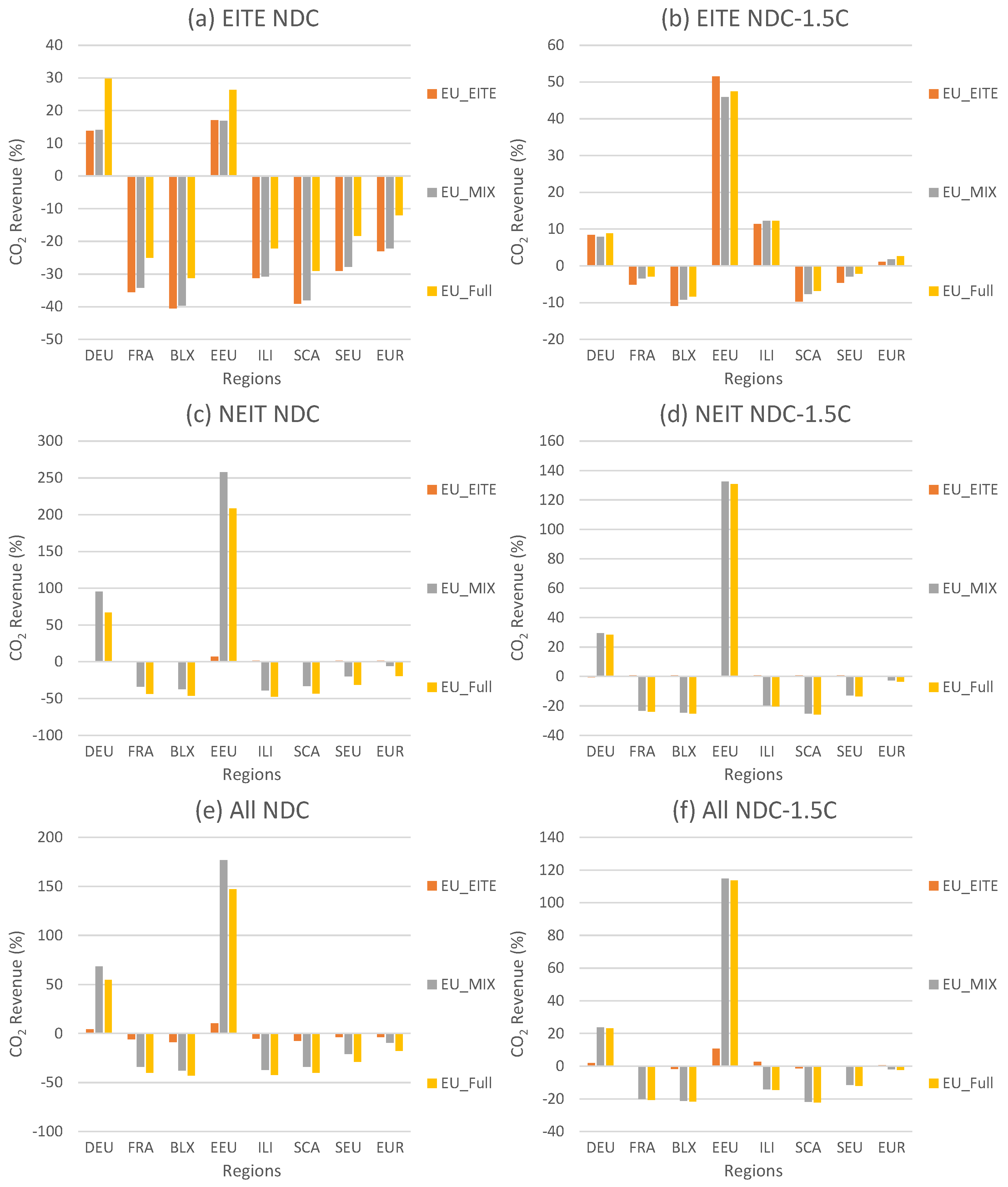
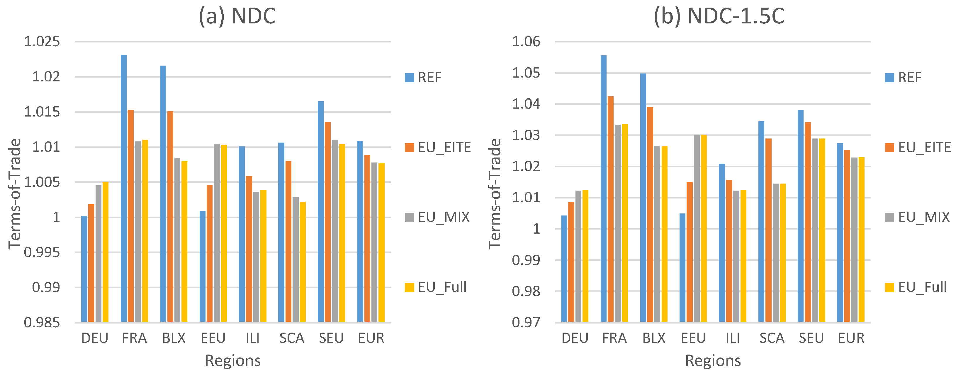
shows the CO₂ prices for the EITE and NEIT sectors, and Figure 6 and Figure 7 present, respectively, the corresponding percentage changes in CO₂ emission and CO₂ revenues in EITE, NEIT, and All sectors. Note that the CO₂ revenues consist of the CO₂ revenues from the internal emission permit market plus the net CO₂ revenues from entering the emission trading markets. The results for import quantity and import price of fuels are reported in

Table 9. Import quantity (M) and import price (PM) of different fuels for different policy scenarios under the NDC target using the IEO baseline.

	REF						EU_EITE
Regions	Coal		Oil		Nat. Gas		Coal		Oil		Nat. Gas
	M	PM	M	PM	M	PM	M	PM	M	PM	M	PM
DEU	−40.7	−10.5	−1.4	−4.1	−28.6	−4.5	−43.4	−10.5	−4.5	−3.9	−31.6	−4.1
FRA	−56.5	−8.6	−27.6	−3.9	−42.3	−5.5	−45.6	−8.4	−20.4	−3.8	−35.1	−5.2
BLX	−68.2	−9.6	−26.8	−4.0	−64.2	−5.2	−59.1	−9.3	−23.1	−3.9	−52.4	−4.9
EEU	−62.1	−12.0	0.3	−4.0	−7.7	−5.9	−82.6	−11.9	−4.5	−3.8	−21.8	−5.7
ILI	−86.6	−11.8	−36.3	−4.0	−71.2	5.1	−75.9	−11.4	−26.3	−3.8	−62.6	5.3
SCA	−79.0	−9.9	−24.1	−4.1	−48.5	−5.8	−69.4	−9.8	−19.0	−3.9	−33.9	−5.6
SEU	−84.3	−10.2	−28.5	−3.9	−42.7	−5.9	−79.3	−10.0	−24.4	−3.8	−36.7	−5.7
EUR	−62.0	−10.2	−19.1	−4.0	−37.5	−5.4	−60.3	−9.9	−17.0	−3.8	−35.3	−5.1
	EU_MIX						EU_Full
Regions	Coal		Oil		Nat. Gas		Coal		Oil		Nat. Gas
	M	PM	M	PM	M	PM	M	PM	M	PM	M	PM
DEU	−49.4	−10.2	−12.0	−4.1	−38.9	−5.2	−48.9	−10.3	−11.6	−4.0	−38.1	−5.5
FRA	−40.3	−8.4	−13.0	−3.8	−28.1	−5.6	−41.9	−8.5	−12.7	−3.7	−27.6	−5.7
BLX	−54.9	−9.3	−13.3	−3.9	−47.4	−5.3	−57.1	−9.3	−12.5	−3.9	−48.6	−5.4
EEU	−85.8	−11.5	−20.2	−4.0	−22.1	−5.8	−86.8	−11.6	−18.5	−4.0	−23.8	−5.9
ILI	−74.9	−11.2	−12.0	−3.8	−57.1	5.3	−77.5	−11.3	−11.1	−3.8	−58.2	5.3
SCA	−67.5	−9.7	−10.5	−4.0	−36.9	−5.8	−70.2	−9.8	−9.5	−4.0	−41.4	−5.8
SEU	−78.4	−9.8	−20.0	−3.8	−33.6	−5.7	−80.0	−9.9	−18.9	−3.8	−33.9	−5.8
EUR	−61.0	−9.7	−15.8	−3.9	−34.3	−5.5	−62.0	−9.8	−14.9	−3.9	−34.6	−5.6

and

Table 10. Import quantity (M) and import price (PM) of different fuels for different policy scenarios under the NDC-1.5C target using the IEO baseline.

	REF						EU_EITE
Regions	Coal		Oil		Nat. Gas		Coal		Oil		Nat. Gas
	M	PM	M	PM	M	PM	M	PM	M	PM	M	PM
DEU	−55.3	−16.0	−18.0	−8.0	−50.3	−6.6	−57.6	−16.2	−22.2	−8.0	−53.1	−6.4
FRA	−70.1	−15.2	−44.6	−7.7	−60.4	−10.6	−67.0	−15.2	−40.4	−7.6	−57.0	−10.5
BLX	−78.8	−16.3	−48.3	−7.8	−78.3	−10.7	−77.3	−16.3	−46.1	−7.8	−72.2	−10.7
EEU	−79.2	−16.8	−4.1	−8.1	−10.5	−12.0	−85.2	−17.0	−12.3	−8.2	−25.3	−12.0
ILI	−89.0	−17.2	−50.3	−6.9	−78.6	1.9	−86.3	−17.2	−44.6	−6.7	−77.3	2.0
SCA	−85.4	−16.9	−41.5	−7.9	−28.3	−12.1	−83.7	−16.9	−36.6	−7.9	−19.8	−12.1
SEU	−89.1	−15.8	−48.8	−7.6	−60.9	−11.7	−88.5	−15.9	−46.9	−7.6	−59.2	−11.7
EUR	−73.2	−16.0	−36.2	−7.8	−53.2	−10.3	−73.6	−16.1	−36.2	−7.8	−53.9	−10.2
	EU_MIX						EU_Full
Regions	Coal		Oil		Nat. Gas		Coal		Oil		Nat. Gas
	M	PM	M	PM	M	PM	M	PM	M	PM	M	PM
DEU	−63.5	−15.6	−29.8	−8.4	−55.7	−7.4	−63.5	−15.7	−29.8	−8.4	−55.7	−7.5
FRA	−60.8	−15.3	−31.2	−7.7	−50.8	−10.7	−60.8	−15.3	−31.2	−7.7	−50.8	−10.7
BLX	−71.8	−16.3	−33.7	−8.0	−68.4	−10.9	−71.8	−16.4	−33.7	−8.0	−68.5	−10.9
EEU	−89.6	−16.1	−39.7	−8.6	−39.5	−12.2	−89.7	−16.2	−39.6	−8.6	−39.6	−12.2
ILI	−85.2	−16.8	−32.3	−7.1	−73.6	1.9	−85.3	−16.8	−32.3	−7.2	−73.5	1.9
SCA	−80.3	−16.8	−23.7	−8.3	−19.4	−12.2	−80.3	−16.8	−23.6	−8.4	−19.9	−12.2
SEU	−87.4	−15.5	−41.8	−7.8	−56.1	−11.8	−87.3	−15.5	−41.8	−7.8	−56.1	−11.8
EUR	−73.9	−15.8	−35.2	−8.1	−53.9	−10.6	−73.9	−15.8	−35.2	−8.1	−54.0	−10.6

. In addition, Figure 8 and Figure 9, respectively, present ToT (Terms-of-Trade in Laspeyres index) and the percentage change in the welfare (measured as equivalent variation (EV) by calculating a composite of representative agent’s consumption) in the selected model regions. EUR shows the aggregated macro indicator or weighted average result for the EU regions in all results. In Figure 7, the results are measured against the REF scenario, whereas in other figures, the results show the changes against the baseline.

In the REF scenario, the regions are restricted to their NDCs (see Table 4 for NDCs), and the carbon prices demonstrate the availability of domestic abatement capacity and the astringency of the ambition level. Nonetheless, the REF scenario’s carbon prices may not precisely match the carbon prices on the MACCs (see Section 2.4), as here, the ToT effects and climate policy in all regions are taken into account. Along with cooperation scenarios, by definition, the CO₂ emissions in regions that do not participate in coalitions do not alter and only change along NDCs. Nevertheless, the carbon prices in regions that do not participate in coalitions can be affected along with the cooperation scenarios, reflecting the ToT effect. The common carbon price will be placed between the highest and the lowest carbon prices in the regions participating in a coalition. Note that the welfare in a participating region is generally affected via: (i) increasing (decreasing) in its carbon emission, (ii) paying (receiving) for emission permits, and (iii) changing its international trade competitiveness.

It is worthwhile first to analyze the results under the REF scenario. The EEU has the lowest carbon price of about 52.9 $/tCO₂ in NDC and about 200.5 $/tCO₂ in NDC-1.5C due to its low MACCs. After the EEU, Germany and SEU, in order, have the lowest carbon price of about 108.9 $/tCO₂ and 313.5 $/tCO₂ in NDC and carbon price of about 458.2 $/tCO₂ and 837.7 $/tCO₂ in NDC-1.5C. France, BLX, ILI, and SCA have significantly higher carbon prices than EEU, Germany, and SEU. The carbon price in France, BLX, ILI, and SCA may go beyond 1000 $/tCO₂ in NDC-1.5C.

Concerning the results under the REF scenario, several insights emerge: (i) Due to the cheaper MACCs in EITE than the MACCs in NEIT, a higher portion of the mitigation is achieved via decreasing the emission in EITE than in NEIT in all model regions and under all ambition levels. (ii) In all regions and under all ambition levels, the import of coal significantly reduces—the import of oil experiences the lowest reduction in the EU as a whole. Under the NDC, the import of oil by EEU even slightly increases. (iii) ToT in all EU regions improves. The ToT improvements are more significant for France, BLX, SCA, and SEU.

Several insights emerge concerning the EU_EITE scenario: (i) The common carbon prices under all ambition levels and baselines are only higher than the EEU’s and Germany’s carbon prices in the REF. Thus, these regions emerge as the suppliers of emission permits. The rest of the regions are the demanders of emission permits. (ii) While the import of fuels by most EU regions increases, the fuel imports decrease in EEU and Germany. Nevertheless, this phenomenon is more visible under the low ambition scenarios. (iii) While the ToT in the EEU and Germany improves, the ToT in the rest of the EU regions degrade. (iv) Forming an emission permit market covering EITE does not significantly influence regional carbon prices in the NEIT sector and only marginally increases them, except for Germany. (v) Except for Germany under the NDC and Germany and EEU under the NDC-1.5C, all the EU regions experience a significant welfare increase, and the welfare in EUR accordingly improves.

In addition, concerning the EU_MIX scenario, several insights emerge: (i) The common carbon price in the emission permit market covering NEIT is significantly higher than the common carbon price in the emission permit market covering EITE. This phenomenon is also influenced by the higher share of emissions in total NEIT from regions with relatively higher carbon prices, such as SEU, which is evident through the aggregate NEIT carbon price in the EUR under the REF scenario (see Table 8 for details). (ii) The formation of the emission permit market covering NEIT does not markedly influence the emission permit market covering EITE, which is evident through insignificant changes in the common carbon prices in the ETS covering EITE sectors in all ambition levels. (iii) EEU and Germany enter the emission permit market covering NEIT as significant emission suppliers permits. Consequently, the overall CO₂ revenues in EEU and Germany rise significantly. The NEIT export reduction in these regions is compensated by the rise in ToT due to the significant decrease in fossil fuel imports. Hence, the welfare in these regions considerably increases. The EEU’s welfare exceptionally improves beyond its baseline level. (iv) Under all ambition levels, France, BLX, ILI, SCA, and SEU demand emission permits covering NEIT, increasing their total emission. However, as the import of fuels significantly increases in these regions, their ToT notably decreases. Nevertheless, it is only under the NDC-1.5C that the effects of emission rise in France and BLX are dominated by the payment and trade effects, and their welfares fall below their REF values. (v) The aggregate import of coal in EUR reduces, whereas the aggregate imports of oil and natural gas increase. The welfare gains in the EEU and Germany outweigh the losses in other regions, and the aggregate welfare in EUR improves.

Finally, concerning the EU_Full scenario, several insights emerge: (i) In all regions, compared to the EU_MIX scenario, mitigation and CO₂ revenues in the EITE sectors increase, while mitigation and CO₂ revenues in the NEIT sectors decrease. Nevertheless, this phenomenon is more pronounced for low than high ambition levels. (ii) Total (All) emissions for all the EU regions do not change significantly. (iii) The overall CO₂ revenues (abatement cost) in all regions and EUR decrease. (v) Under the NDC, due to a further reduction in coal production, the EU regions become more dependent on imported oil. Under the NDC-1.5C, the composition of fossil fuel imports does not alter. Nevertheless, the ToT in the EU regions does not significantly change. (vi) All the EU regions under the low ambition levels experience a remarkable welfare loss. Nevertheless, such a welfare reduction is less significant under the high ambition levels. (vii) In the EEU, the welfare under EU_Full is still significantly higher than that under the REF scenario. In addition, (viii) while EUR under the EU_Full scenario has significantly higher welfare than the REF scenario, the aggregate welfare is slightly lower than that under the EU_EITE. However, the EUR welfare is greater than the EU_EITE under the high ambition levels but still slightly lower than the EU_MIX scenario.

3.4. Policy Scenarios under the WEO Baseline

This section compares the results of policy scenarios using the WEO baseline with the IEO baseline results. The results are presented as percentage change against the IEO baseline results. For the sake of brevity, only selected results are presented under the NDC ambition level. Figure 10 shows the corresponding percentage changes in CO₂ emission and CO₂ revenues in the EITE, NEIT, and All sectors in the EU regions. In addition, Figure 11 shows the percentage changes in ToT and welfare in the EU regions. For the comparison, absolute values of absolute CO₂ emissions, CO₂ revenues, ToT, and welfare are compared to get the percentage changes. Therefore, the baselines value and ambition levels are simultaneously taken into account.

Several insights emerge: (i) The absolute emissions under the WEO baseline in all regions in the REF scenario are less than the IEO, even though the NDC ambition levels under the WEO scenario are less ambitious than the IEO scenario for all regions, except for SCA. This is because the baseline emission factor in 2030 under the WEO baseline is less than that under the IEO baseline, except for SCA (see Figure 3). (ii) The aggregate percentage reduction in NEIT emission in EUR is more than that in the EITE emission in the REF scenario. (iii) Except for SEU and ILI, all the EU regions experience emission reduction in their EITE and NEIT sectors in the REF scenario—EITE emissions in SEU significantly increase, and NEIT emissions in ILI slightly increase. (iv) The emission pattern holds for all regions under all scenarios, except for ILI and SCA, whose total emission under the WEO baseline can be higher than that under the IEO baseline. (v) Due to the substantial increase in REF carbon prices in SCA and ILI, their CO₂ revenues increase. For the rest of the regions, the CO₂ revenues decrease. (vi) In the REF scenario, the ToTs under the WEO baseline are degraded in all regions except BLX and SCA. Nevertheless, (vii) the lower abatement cost dominates the effects, and all EU regions have higher welfare under the WEO baseline than under the IEO baseline. Note that since the percentage changes in welfare are close, the conclusion that the EU regions have more welfare under the EU_MIX scenario than that under the EU_Full holds.

3.5. Additional Scenarios

This subsection presents the results of two different scenarios to help better understand the international trade effects with the policy scenarios in the previous subsection. The scenarios are described in Table 6. Figure 12 presents the corresponding percentage changes in CO₂ emission and CO₂ revenues in the EITE, NEIT, and ALL sectors in the EU regions. The results on CO₂ revenues are measured against the REF scenario. In addition, Figure 13 shows ToT and the percentage change in the welfare in the EU regions.

Several insights emerge concerning the NO_ROW scenario: (i) While the combination of abatement in the EU does not depend on climate policy in other regions, the CO₂ revenue reduction reveals that no climate policy in other regions implies a lower carbon price for the EU regions. This is due to the higher import price of fuels. (ii) Only ToT in Germany slightly increases, whereas ToT for the rest of the EU regions decreases. (iii) Due to the reduced cost of achieving the NDC target under No_ROW, most EU regions, except for ILI, experience an improvement in their welfare.

Regarding the No_EUR scenario, the results imply the following: (i) There can be a significant emission leakage to the EU regions due to the lower global price of fossil fuels—the aggregate emission in the EU rises by about 7%. Such leakage is more pronounced in the EITE sectors than in the NEIT. (ii) France, BLX, ILI, SCA, and SEU experience a significant reduction in their ToT compared to the baseline. ToT in Germany and EEU are not greatly affected. (iii) Compared to the baseline, the welfare effect for all the EU regions, except for ILI, is negative.

4. Discussion

4.1. The Emission Trading Flexibility of Europe

For a correct comparison of the results in this paper with the EMF36 Core results, in which Europe is not disaggregated (see Böhringer et al. [6]), three points must be taken into account. First, a complete aggregation of Europe in the EMF36 Core scenarios would mean perfect cooperation between European regions, including REU and GBR, which are no longer participating in the EU ETS. Second, the benchmark scenario is calibrated using the GTAP 10 Power data set [27,28] in this paper, whereas EMF36 Core harmonization was built on GTAP 9 [21]. Third, the NDCs ambition levels in this paper are updated using the latest submitted promises, which mean more ambitious targets for the EU. Considering these points, one realizes that the aggregate welfare loss in the REF scenario reported under the EUR region in this paper is only slightly higher than the REF’s mean welfare loss in the EMF36 Core project (see Figure 5 in Böhringer et al. [6]). Therefore, this study benefits from updated data and further disaggregation, which creates a higher possibility for efficiently reallocating emission abatement.

There are different interpretations of NDCs than those used in this paper (see Chepeliev and van der Mensbrugghe [45]). Most likely, applying different NDC interpretations will generate different results. Note that a different ambition level in a region outside the EU can still affect the outcomes for European regions when employing a multi-regional CGE model. Therefore, the interpretation of the results in this study must consider this point. Nevertheless, this paper shows that the climate policy in other regions does not change the results qualitatively. Therefore, the results in this paper indicated that the general results qualitatively hold should different NDC interpretations being used. In this regard, the No_ROW scenario can be qualitatively similar to increased ambitions in the regions participating in the EU ETS, while the rest of the model regions have not elevated their mitigation targets.

An extra note on baseline choice is in place. While the results using the IEO and WEO baselines show differences, these baselines have similarities that could be different in other baselines. Notably, several regions provide emission baselines different from the IEO and WEO baselines. In addition, countries such as China and India still have significantly low commitments in this paper after the updated obligations are taken into account. However, as there is pressure on these countries for accelerating their abatement efforts, the effect through international trade could affect other regions, including the EU. So, extra care is needed to interpret the results in this paper regarding a baseline choice.

The technological representations in the model strictly follow the representations in the GTAP 10 Power data set. Comparing the results in this paper with the EMF36 Core projects can show a meaningful change due to the updated data. Nevertheless, there are no backstop technologies in the forward calibration of the model or counterfactual scenarios, which may impact the results. In this regard, the results, especially on the CO₂ prices, must be regarded as the upper bound.

This article does not implement revenue redistribution scenarios. Nevertheless, this paper conducts a “search” technique to specify opportunities for welfare gains. In this regard, under the NDC, NDC+, and NDC-2C ambition levels, the EU_MIX scenario achieves higher aggregate welfare than REF, and all the EU regions would gain welfare even without any redistribution method applied. To this end, both stability and self-enforcing characteristics can be achieved via the parallel emission tradings. All in all, future studies for investigating different redistribution schemes for coalitions with parallel emission trading links are recommended.

4.2. The Emission Trading Flexibility and Innovation in Environmental Industry

In this article, two aspects are related to innovations in mitigation technology. Firstly, the improvements in the productivity and energy efficiency in the baseline can be considered exogenous innovations. Nevertheless, such innovations are currently limited to the baseline and do not enhance further in policy scenarios. Future studies should address this issue through the endogenous implementation of productivity and energy efficiency based on the incentives provided by the carbon price. Second, the new market design can span the cost-effective options to reach the mitigation goals. In this regard, while a specific sector may find the carbon price a solid incentive to trigger research and development for innovative mitigation approaches, the chances are that further emission trading flexibility strengthens the incentives due to the extra carbon revenues. In this paper, only two parallel emission markets have been studied. Future research may explore more markets with various sector combinations.

Some studies recommend that a carbon price is the only policy intervention required for climate preservation [46], and additional policy measures concerning climate or technology may decrease the climate policy effectiveness [47]. The argument for utilizing carbon pricing as the prominent policy instrument is that polluters have an economic incentive to immediately reduce their emissions, activating the development and deployment of lower-emitting technologies [48]. While many regard the growing number of countries implementing carbon pricing as proof of success [49], some studies indicate that such policies have not activated significant abatement [50].

Substantial learning-by-doing effects and increasing returns to scale are featured with new and novel clean technologies (e.g., batteries and low-carbon energy storage technologies) [51]. Studies indicate that average solar PV module costs may fall by about 20% each time the cumulative installed capacity doubles [52]. Therefore, additional policies (e.g., feed-in tariffs and standards) can be justified mechanisms for incentivizing innovations and investments to reach the potential increasing returns [53]. The incandescent lightbulb ban in Europe is a compelling example—it resulted in the deployment of LED lightbulbs at lower costs and with higher quality and efficiency than the incandescent equivalent [54,55]. Note that the effectiveness of policies depends on many factors, including the influential mechanisms of power actor groups (see Mohammadi and Khabbazan [56] for a comparison of feed-in tariffs in the renewable energy transition in Iran and Germany).

While the “conventional wisdom” is that the first-best carbon price is globally uniform, Stiglitz [57] shows that carbon prices may differ across time, over space, and with various uses. Therefore, this article’s results conform with the results by Stiglitz [57] and show that parallel ETSs may be more efficient than an ETS covering all sectors and countries. Indeed, if concerns about innovation, distribution, and uncertainty are appropriately incorporated into the analysis, this finding properly lies within the standard modern public finance theory [53,57]. By numerically modeling the possibility of differentiated simultaneous emission trading markets in the EU, this article quantifies a prototpical setup with multiple ETSs subject to various policy scenarios. Hence, this article brings insights into current proposals’ distributional effects and cost-effectiveness.

Concerning a zero-emission goal, policies to incentivize technologies such as those that remove greenhouse gases from the atmosphere are crucial and must be incentivized by adequate policies [58]. For this reason, carbon pricing incentivizing CO₂ removals has a substantial role which should be distinguished from only disincentivizing CO₂ emissions [53]—in this regard, emission trading system may provide appropriate incentives.

5. Conclusions

Through the Paris Agreement, individual countries, including European countries, have submitted national pledges of specific reductions in their carbon emissions by 2030, so-called Nationally Determined Contributions (NDCs). These NDCs can be met through different instruments such as carbon pricing and emission trading systems (ETS). The EU has established the world’s first cross-border ETS for greenhouse gas (GHG) emissions, currently covering aviation, emission-intensive sectors, and electricity (EITE).

To achieve the 2030 target, the EU Commission has suggested applying emissions trading in new sectors where sharper mitigations are needed. Under the proposition, emissions from maritime transport will be incorporated into the current EU ETS, while a separate emissions trading system will cover emissions from fuels utilized in road transport and the building sector. In response to the EU Commission’s suggestion, this article presents insights into the merits of alternative design options for greenhouse gas emissions trading in the EU, focusing on variations in the coverage of relevant sectors.

In this study, a multi-regional multi-sectoral CGE model is applied to operate with the option of forming two international emission permit markets simultaneously. Using the GTAP 10 Power data set, the EU region is aggregated into nine regions, including two individual countries (Germany and France) and seven aggregated regions. Then, after forward-calibration of the model based on International Energy Outlook (IEO) and World Energy Outlook (WEO) projections until 2030, marginal abatement cost curves (MACCs) are derived. Moreover, besides the REF scenario in which no region collaborates, three policy scenarios are simulated: (i) EU_EITE as an ETS covering the EITE, mimicking the current EU ETS sectors, (ii) EU_MIX where, in addition to an ETS covering EITE, another ETS covers the sectors other than EITE (NEIT), and (iii) EU_Full, where one ETS covers all sectors. In addition, two different scenarios are simulated where either only the EU or the rest of the model regions implement their climate policy. Each scenario is run for four emission reduction targets, i.e., post-2020 Nationally Determined Contributions (NDC), conditional NDC (NDC+), NDC to meet the 2-degree global average temperature target (NDC-2C), and NDC to meet the 1.5-degree global average temperature target (NDC-1.5C).

The results show that between 44.2% (Germany) and 70.2% (France) of the emissions are made by burning fossil fuels in the NEIT sectors in these regions under the IEO baseline. Emissions by the NEIT sectors are significantly higher under the WEO baseline than under the IEO baseline in all the EU regions, except for South Europe (SEU). Moreover, the results on MACCs indicate that NEIT MACCs are more expensive than EITE MACCs under both baselines. In addition, East Europe (EEU) and Germany have the lowest MACCs among the EU regions, whereas France, BLX, and SCA have the highest MACCs. Additionally, the MACCs under the WEO baseline are slightly higher than under the IEO baseline.

Policy scenarios show that in the REF scenario, more abatement is done via decreasing the emission in the EITE than in the NEIT. In addition, in the EU_EITE scenario, France, BLX, ILI, SCA, and SEU take the emission permit demander position. Hence, EITE emissions in these regions increase, whereas EEU and Germany supply emission permits. Except for Germany, all the participating regions in the emission permit market covering EITE sectors (EU_EITE) gain welfare under NDC, NDC+, and NDC-2C ambition levels. Concerning the EU_MIX scenario, the results show that the common carbon price in the emission permit market covering the NEIT is significantly higher than the common carbon price in the emission permit market covering the EITE. All EU regions gain welfare compared to the REF scenario under the EU_MIX scenario in NDC, NDC+, and NDC-2C—the EU_MIX is stable and self-enforcing. The welfare gain under the EU_MIX in EEU is so significant that its welfare improves significantly beyond its baseline value. The aggregate welfare in the EU further enhances under the EU_MIX scenario against the EU_EITE scenario. Additionally, due to a reduction in coal production, the EU regions become more dependent on importing oil under the EU_Full. Accordingly, the welfare in all EU regions decreases against the EU_MIX. This phenomenon is more significant under the low ambition levels.

Moreover, the results show that the climate policy in other regions does not significantly affect the EU regions’ welfare. Furthermore, the results reveal that baseline choice can affect the results—the CO₂ revenues are considerably lower in all EU regions except for ILI and SCA, and welfare in all regions significantly increases using the WEO baseline than the IEO baseline. Nevertheless, the changes in welfare along the different policy scenarios are insignificant, and hence, the results qualitatively hold regardless of the baseline choice.

References

1. Ostrom, E. A multi-scale approach to coping with climate change and other collective action problems. Solutions 2010, 1, 27–36. [Google Scholar]
2. UNFCCC. Paris Agreement. Available online: https://unfccc.int/sites/default/files/english_paris_agreement.pdf (accessed on 28 April 2022).
3. UNFCCC. NDC Registry. Available online: https://www4.unfccc.int/sites/NDCStaging/Pages/All.aspx (accessed on 28 April 2022).
4. Akın-Olçum, G.; Ghosh, M.; Gilmore, E.; Johnston, P.; Khabbazan, M.M.; Lubowski, R.; McCallister, M.; Macaluso, N.; Peterson, S.; Winkler, M.; et al. A model intercomparison of the welfare effects of regional cooperation for ambitious climate mitigation targets. In Proceedings of the 26th Annual Conference of the European Association of Environmental and Resource Economists, Online, 23–25 June 2021. [Google Scholar]
5. Alexeeva, V.; Anger, N. The globalization of the carbon market: Welfare and competitiveness effects of linking emissions trading schemes. Mitig. Adapt. Strateg. Glob. Chang. 2016, 21, 905–930. [Google Scholar] [CrossRef]
6. Böhringer, C.; Peterson, S.; Rutherford, T.F.; Schneider, J.; Winkler, M. Climate policies after Paris: Pledge, Trade and Recycle: Insights from the 36th Energy Modeling Forum Study (EMF36). Energy Econ. 2021, 103, 105471. [Google Scholar] [CrossRef]
7. Fujimori, S.; Kubota, I.; Dai, H.; Takahashi, K.; Hasegawa, T.; Liu, J.Y.; Hijioka, Y.; Masui, T.; Takimi, M. Will international emissions trading help achieve the objectives of the Paris Agreement? Environ. Res. Lett. 2016, 11, 104001. [Google Scholar] [CrossRef]
8. Nong, D.; Siriwardana, M. The most advantageous partners for Australia to bilaterally link its emissions trading scheme. Int. J. Glob. Warm. 2018, 15, 371–391. [Google Scholar] [CrossRef]
9. Stiglitz, J.; Stern, N.; Duan, M.; Edenhofer, O.; Giraud, G.; Heal, G.; la Rovere, E.; Morris, A.; Moyer, E.; Pangestu, M.; et al. High-Level Commission on Carbon Prices. 2017. Report of the High-Level Commission on Carbon Prices. Washington, DC: World Bank. License: Creative Commons Attribution CC BY 3.0 IGO. Available online: https://static1.squarespace.com/static/54ff9c5ce4b0a53decccfb4c/t/59244eed17bffc0ac256cf16/1495551740633/CarbonPricingFinalMay29.pdf (accessed on 28 April 2022).
10. Flachsland, C.; Marschinski, R.; Edenhofer, O. To link or not to link: Benefits and disadvantages of linking cap-and-trade systems. Clim. Policy 2009, 9, 358–372. [Google Scholar] [CrossRef]
11. Khabbazan, M.M.; von Hirschhausen, C. The implication of the Paris targets for the Middle East through different cooperation options. Energy Econ. 2021, 104, 105629. [Google Scholar] [CrossRef]
12. Paltsev, S.V. The Kyoto Protocol: Regional and sectoral contributions to the carbon leakage. Energy J. 2001, 22, 53–80. [Google Scholar] [CrossRef] [Green Version]
13. Peterson, S.; Weitzel, M. Reaching a climate agreement: Compensating for energy market effects of climate policy. Clim. Policy 2016, 16, 993–1010. [Google Scholar] [CrossRef]
14. Barrett, S. Environment and Statecraft: The Strategy of Environmental Treaty-Making; OUP Oxford: New York, NY, USA, 2003. [Google Scholar]
15. Böhringer, C.; Carbone, J.C.; Rutherford, T.F. The strategic value of carbon tariffs. Am. Econ. J. Econ. Policy 2016, 8, 28–51. [Google Scholar] [CrossRef] [Green Version]
16. Lessmann, K.; Kornek, U.; Bosetti, V.; Dellink, R.; Emmerling, J.; Eyckmans, J.; Nagashima, M.; Weikard, H.P.; Yang, Z. The stability and effectiveness of climate coalitions. Environ. Resour. Econ. 2015, 62, 811–836. [Google Scholar] [CrossRef] [Green Version]
17. European Commission. 2030 Climate and Energy Framework. Available online: https://ec.europa.eu/clima/eu-action/climate-strategies-targets/2030-climate-energy-framework_en (accessed on 28 April 2022).
18. Tol, R.S. Intra-union flexibility of non-ETS emission reduction obligations in the European Union. Energy Policy 2009, 37, 1745–1752. [Google Scholar] [CrossRef] [Green Version]
19. Böhringer, C. Two decades of European climate policy: A critical appraisal. Rev. Environ. Econ. Policy 2014, 8, 1–17. [Google Scholar] [CrossRef]
20. Vielle, M. Navigating various flexibility mechanisms under European burden-sharing. Environ. Econ. Policy Stud. 2020, 22, 267–313. [Google Scholar] [CrossRef]
21. Aguiar, A.; Narayanan, B.; McDougall, R. An overview of the GTAP 9 data base. J. Glob. Econ. Anal. 2016, 1, 181–208. [Google Scholar] [CrossRef]
22. Faehn, T.; Yonezawa, H. Emission targets and coalition options for a small, ambitious country: An analysis of welfare costs and distributional impacts for Norway. Energy Econ. 2021, 103, 105607. [Google Scholar] [CrossRef]
23. Landis, F.; Fredriksson, G.; Rausch, S. Between- and within-country distributional impacts from harmonizing carbon prices in the EU. Energy Econ. 2021, 103, 105585. [Google Scholar] [CrossRef]
24. Winkler, M.B.J.; Peterson, S.; Thube, S. Gains associated with linking the EU and Chinese ETS under different assumptions on restrictions, allowance endowments, and international trade. Energy Econ. 2021, 104, 105630. [Google Scholar] [CrossRef]
25. Kriegler, E.; Gulde, R.; Colell, A.; von Hirschhausen, C.; Minx, J.C.; Oei, P.Y.; Yanguas-Parra, P.; Bauer, N.; Brauers, H.; Broska, L.H.; et al. Phasing Out Fossil Fuels—How to Achieve a Just Transition? Background Paper for the Forum Climate Economics 7; Federal Ministry for Education and Research (BMBF): Berlin, Germany, 2020. [Google Scholar]
26. European Commission. Questions and Answers—Emissions Trading—Putting a Price on carbon. Available online: https://ec.europa.eu/commission/presscorner/detail/en/qanda_21_3542 (accessed on 29 April 2022).
27. Aguiar, A.; Chepeliev, M.; Corong, E.; McDougall, R.; van der Mensbrugghe, D. The GTAP Data Base: Version 10. J. Glob. Econ. Anal. 2019, 4, 1–27. [Google Scholar] [CrossRef] [Green Version]
28. Chepeliev, M. GTAP-Power Data Base: Version 10. J. Glob. Econ. Anal. 2020, 5, 110–137. [Google Scholar] [CrossRef]
29. EIA. International Energy Outlook 2017; U.S. Energy Information Administration: Washington, DC, USA, 2017. [Google Scholar]
30. IEA. World Energy Outlook 2018; International Energy Agency: Paris, France, 2018. [Google Scholar]
31. Anger, N. Emissions trading beyond Europe: Linking schemes in a post-Kyoto world. Energy Econ. 2008, 30, 2028–2049. [Google Scholar] [CrossRef]
32. Carbone, J.C.; Helm, C.; Rutherford, T.F. The case for international emission trade in the absence of cooperative climate policy. J. Environ. Econ. Manag. 2009, 58, 266–280. [Google Scholar] [CrossRef] [Green Version]
33. Mehling, M.A.; Metcalf, G.E.; Stavins, R.N. Linking climate policies to advance global mitigation. Science 2018, 359, 997–998. [Google Scholar] [CrossRef] [PubMed] [Green Version]
34. Doda, B.; Quemin, S.; Taschini, L. Linking permit markets multilaterally. J. Environ. Econ. Manag. 2019, 98, 102259. [Google Scholar] [CrossRef]
35. Holtsmark, B.; Weitzman, M.L. On the Effects of Linking Cap-and-Trade Systems for CO2 Emissions. Environ. Resour. Econ. 2020, 75, 615–630. [Google Scholar] [CrossRef] [Green Version]
36. Lanz, B.; Rutherford, T.F. GTAPinGAMS: Multiregional and small open economy models. J. Glob. Econ. Anal. 2016, 1, 1–77. [Google Scholar] [CrossRef]
37. Böhringer, C.; Rutherford, T.F. The costs of compliance: A CGE assessment of Canada’s policy options under the Kyoto protocol. World Econ. 2010, 33, 177–211. [Google Scholar] [CrossRef]
38. Armington, P.S. A theory of demand for products distinguished by place of production. Staff Pap. 1969, 16, 159–178. [Google Scholar] [CrossRef]
39. Brooke, A.; Kendrick, D.; Meeraus, A.; Raman, R. GAMS, a User’s Guide, 1998; GAMS Development Corporation: Washington, DC, USA, 1998. [Google Scholar]
40. Dirkse, S.P.; Ferris, M.C. The PATH solver: A nommonotone stabilization scheme for mixed complementarity problems. Optim. Methods Softw. 1995, 5, 123–156. [Google Scholar] [CrossRef]
41. Beckman, J.; Hertel, T.; Tyner, W. Validating energy-oriented CGE models. Energy Econ. 2011, 33, 799–806. [Google Scholar] [CrossRef] [Green Version]
42. Okagawa, A.; Ban, K. Estimation of Substitution Elasticities for CGE Models; Discussion Papers in Economics and Business; Graduate School of Economics, Osaka University: Osaka, Japan, 2008. [Google Scholar]
43. Faehn, T.; Bachner, G.; Beach, R.; Chateau, J.; Fujimori, S.; Ghosh, M.; Hamdi-Cherif, M.; Lanzi, E.; Paltsev, S.; Vandyck, T.; et al. Capturing Key Energy and Emission Trends in CGE models: Assessment of Status and Remaining Challenges. J. Glob. Econ. Anal. 2020, 5, 196–272. [Google Scholar] [CrossRef]
44. Foure, J.; Aguiar, A.; Bibas, R.; Chateau, J.; Fujimori, S.; Lefevre, J.; Leimbach, M.; Rey-Los-Santos, L.; Valin, H. Macroeconomic drivers of baseline scenarios in dynamic CGE models: Review and guidelines proposal. J. Glob. Econ. Anal. 2020, 5, 28–62. [Google Scholar] [CrossRef]
45. Chepeliev, M.; van der Mensbrugghe, D. Global fossil-fuel subsidy reform and Paris Agreement. Energy Econ. 2020, 85, 104598. [Google Scholar] [CrossRef]
46. Blum, J.; de Britto Schiller, R.; Löschel, A.; Pfeiffer, J.; Pittel, K.; Potrafke, N.; Schmitt, A. Zur Bepreisung von CO2-Emissionen–Ergebnisse aus dem Ökonomenpanel. Ifo Schnelld. 2019, 72, 60–65. [Google Scholar]
47. Nordhaus, W.D. The Climate Casino: Risk, Uncertainty, and Economics for a Warming World; Yale University Press: New Haven, CT, USA, 2013. [Google Scholar]
48. Lilliestam, J.; Patt, A.; Bersalli, G. The effect of carbon pricing on technological change for full energy decarbonization: A review of empirical ex-post evidence. Wiley Interdiscip. Rev. Clim. Chang. 2021, 12, e681. [Google Scholar] [CrossRef]
49. Ramstein, C.; Dominioni, G.; Ettehad, S.; Lam, L.; Quant, M.; Zhang, J.; Mark, L.; Nierop, S.; Berg, T.; Leuschner, P.; et al. State and Trends of Carbon Pricing 2019; The World Bank: Washington, DC, USA, 2019. [Google Scholar]
50. Haites, E. Carbon taxes and greenhouse gas emissions trading systems: What have we learned? Clim. Policy 2018, 18, 955–966. [Google Scholar] [CrossRef] [Green Version]
51. Farmer, J.D.; Lafond, F. How predictable is technological progress? Res. Policy 2016, 45, 647–665. [Google Scholar] [CrossRef] [Green Version]
52. de La Tour, A.; Glachant, M.; Ménière, Y. Predicting the costs of photovoltaic solar modules in 2020 using experience curve models. Energy 2013, 62, 341–348. [Google Scholar] [CrossRef]
53. Hepburn, C.; Stern, N.; Stiglitz, J.E. “Carbon pricing” special issue in the European economic review. Eur. Econ. Rev. 2020, 127, 103440. [Google Scholar] [CrossRef]
54. European Commission. 2009. FAQ: Phasing out Conventional Incandescent Bulbs. Available online: https://europa.eu/rapid/press-release_MEMO-09-368_en.htm (accessed on 30 April 2022).
55. UN Environment. Accelerating the Global Adoption of Energy-Efficient Lighting. 2017. Available online: http://united4efficiency.org/wp-content/uploads/2017/04/U4E-LightingGuide-201703-Final.pdf (accessed on 30 April 2022).
56. Mohammadi, N.; Khabbazan, M.M. The Influential Mechanisms of Power Actor Groups on Policy Mix Adoption: Lessons Learned from Feed-In Tariffs in the Renewable Energy Transition in Iran and Germany. Sustainability 2022, 14, 3973. [Google Scholar] [CrossRef]
57. Stiglitz, J.E. Addressing climate change through price and non-price interventions. Eur. Econ. Rev. 2019, 119, 594–612. [Google Scholar] [CrossRef]
58. Hepburn, C.; Adlen, E.; Beddington, J.; Carter, E.A.; Fuss, S.; Mac Dowell, N.; Minx, J.C.; Smith, P.; Williams, C.K. The technological and economic prospects for CO2 utilization and removal. Nature 2019, 575, 87–97. [Google Scholar] [CrossRef] [PubMed] [Green Version]
Figure 1. Nesting structure in non-fossil fuel production [11].
Joitmc 08 00091 g001
Figure 2. Nesting structure in fossil fuel production [11].
Joitmc 08 00091 g002
Figure 3. CO2 scales and GDP scales for the IEO and WEO baselines in 2014–2030 (used for calibration).
Joitmc 08 00091 g003
Figure 4. EITE, NEIT, and ALL MACCs in percentage change for different European regions in 2030 under the IEO and WEO baselines.
Joitmc 08 00091 g004
Figure 5. EITE, NEIT, and All MACCs in percentage change in EUR in 2030 under the IEO and WEO baselines.
Joitmc 08 00091 g005
Figure 6. Percentage change in CO2 emission in EITE, NEIT, and ALL sectors for different policy scenarios and NDCs using the IEO baseline.
Joitmc 08 00091 g006
Figure 7. Percentage change in CO2 revenues in EITE, NEIT, and ALL sectors with regard to CO2 revenues in the REF scenario for different policy scenarios and NDCs using the IEO baseline.
Joitmc 08 00091 g007
Figure 8. Terms-of-trade in the EU regions for different policy scenarios and NDCs using the IEO baseline.
Joitmc 08 00091 g008
Figure 9. Percentage change in welfare for different policy scenarios and NDCs using the IEO baseline.
Joitmc 08 00091 g009
Figure 10. Percentage change in CO2 emission and CO2 revenues for different policy scenarios using the WEO baseline against the IEO baseline.
Joitmc 08 00091 g010
Figure 11. Percentage change in ToT and wefare for different policy scenarios using the WEO baseline against the IEO baseline.
Joitmc 08 00091 g011
Figure 12. Percentage change in emission and CO2 revenues in EITE, NEIT, and ALL sectors for different scenarios using the IEO baseline.
Joitmc 08 00091 g012
Figure 13. ToT and percentage change in welfare for different scenarios using the IEO baseline.
Joitmc 08 00091 g013