Article

A Novel Enhanced Differential Evolution Algorithm for Outbound Logistics of the Poultry Industry in Thailand

1
Research Unit on System Modelling for Industry, Department of Industrial Engineering, Faculty of Engineering, Khon Kaen University, Khon Kaen 40002, Thailand
2
Faculty of Business Administration and Accountancy, Khon Kaen University, Khon Kaen 40002, Thailand
*
Author to whom correspondence should be addressed.
J. Open Innov. Technol. Mark. Complex. 2022, 8(1), 15; https://doi.org/10.3390/joitmc8010015
Submission received: 23 October 2021 / Revised: 30 December 2021 / Accepted: 31 December 2021 / Published: 10 January 2022

Abstract

:
Outbound logistics is a crucial field of logistics management. This study considers a planning distribution for the poultry industry in Thailand. The goal of the study is to minimize the transportation cost for the multi-depot vehicle-routing problem (MDVRP). A novel enhanced differential evolution algorithm (RI-DE) is developed based on a new re-initialization mutation formula and a local search function. A mixed-integer programming formulation is presented in order to measure the performance of a heuristic with GA, PSO, and DE for small-sized instances. For large-sized instances, RI-DE is compared to the traditional DE algorithm for solving the MDVRP using published benchmark instances. The results demonstrate that RI-DE obtained a near-optimal solution of 99.03% and outperformed the traditional DE algorithm with a 2.53% relative improvement, not only in terms of solution performance, but also in terms of computational time.

1. Introduction

In recent years, competitive markets, challenging customer demands, and increased awareness of logistics and transportation activities have increased the importance of technology for Thailand’s poultry industry. In order to develop new technology for the marketplace, companies “can and should use external ideas and internal ideas, as well as internal and external paths to market,” according to the open innovation paradigm [1]. In addition to logistics management being influenced by innovations, new technologies are evolving in response to businesses’ goals and competitiveness conditions, increasing their complexity [2]. Currently, logistics, also known as logistics 4.0, is receiving the most attention in the fourth industrial revolution trend. Artificial intelligence, real-time tracking, data-driven network logistics, the internet of things, optimization software, and so on are examples of technologies [3,4,5]. These logistics 4.0 technologies will significantly impact Thailand’s poultry industry’s outbound logistics planning.
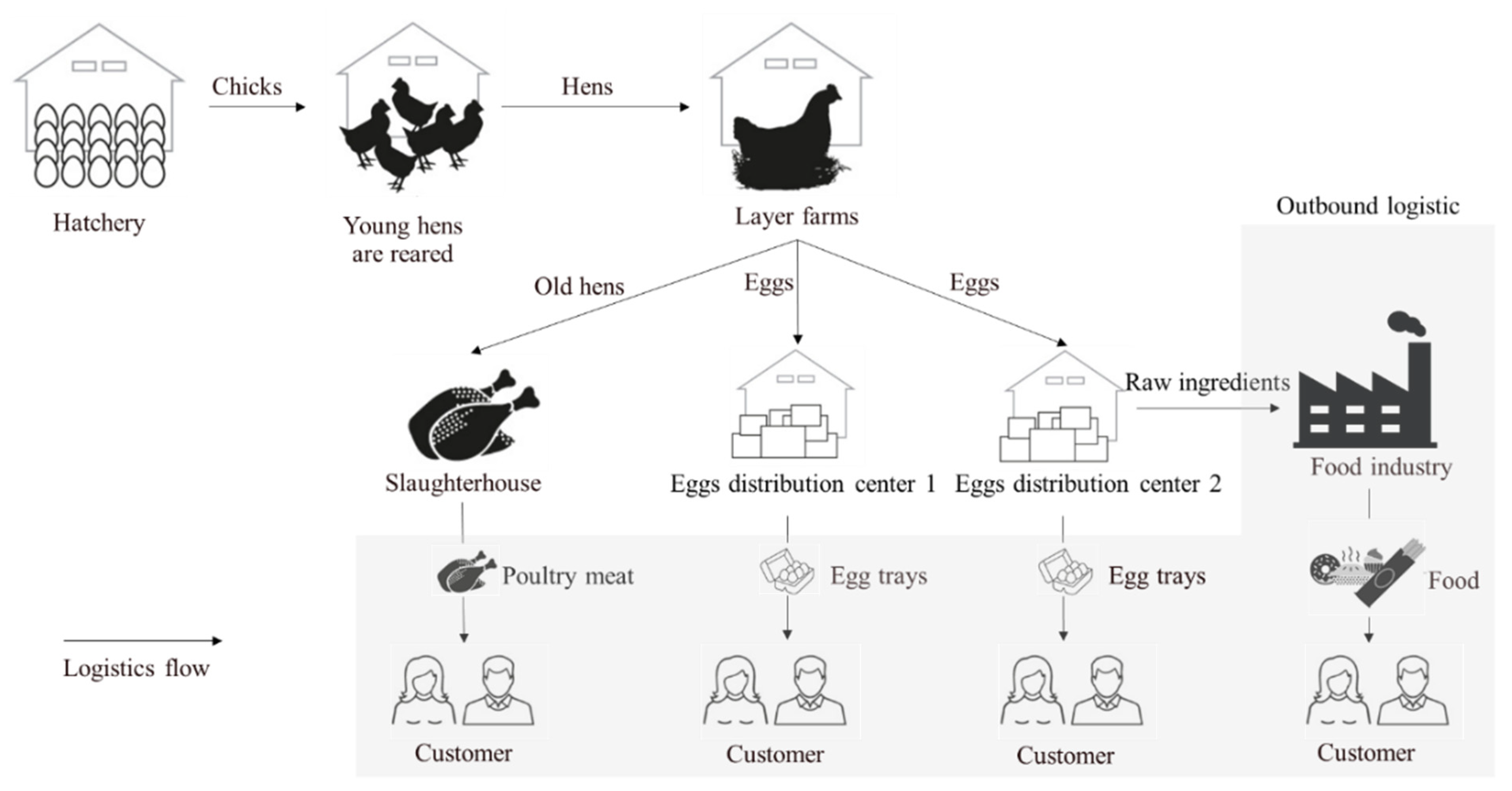
The outbound logistics of the poultry industry in Thailand are considered in this paper, as agricultural products comprise a significant part of Thailand’s development, impacting Thailand’s economic growth. Outbound logistics is the shipping of finished products to customers from a distribution center. At this stage, transportation is typically carried out by trucks. Distribution planning can be a challenging problem and adhering to distribution center best practices is also crucial for ensuring the efficient transportation of products. The importance of poultry distribution planning has increased, due to rising transportation costs and opportunities for decreasing costs in incorporating optimal distribution planning. A flow process of outbound logistics for the poultry industry in Thailand is depicted in Figure 1. In short, the outbound logistics of the poultry industry in Thailand consists of three principal distributions: (1) The old hens are slaughtered and then sold as poultry meats to customers; (2) eggs are mainly sold directly to the end-consumers; and (3) broken eggs are sent to a processing plant [6,
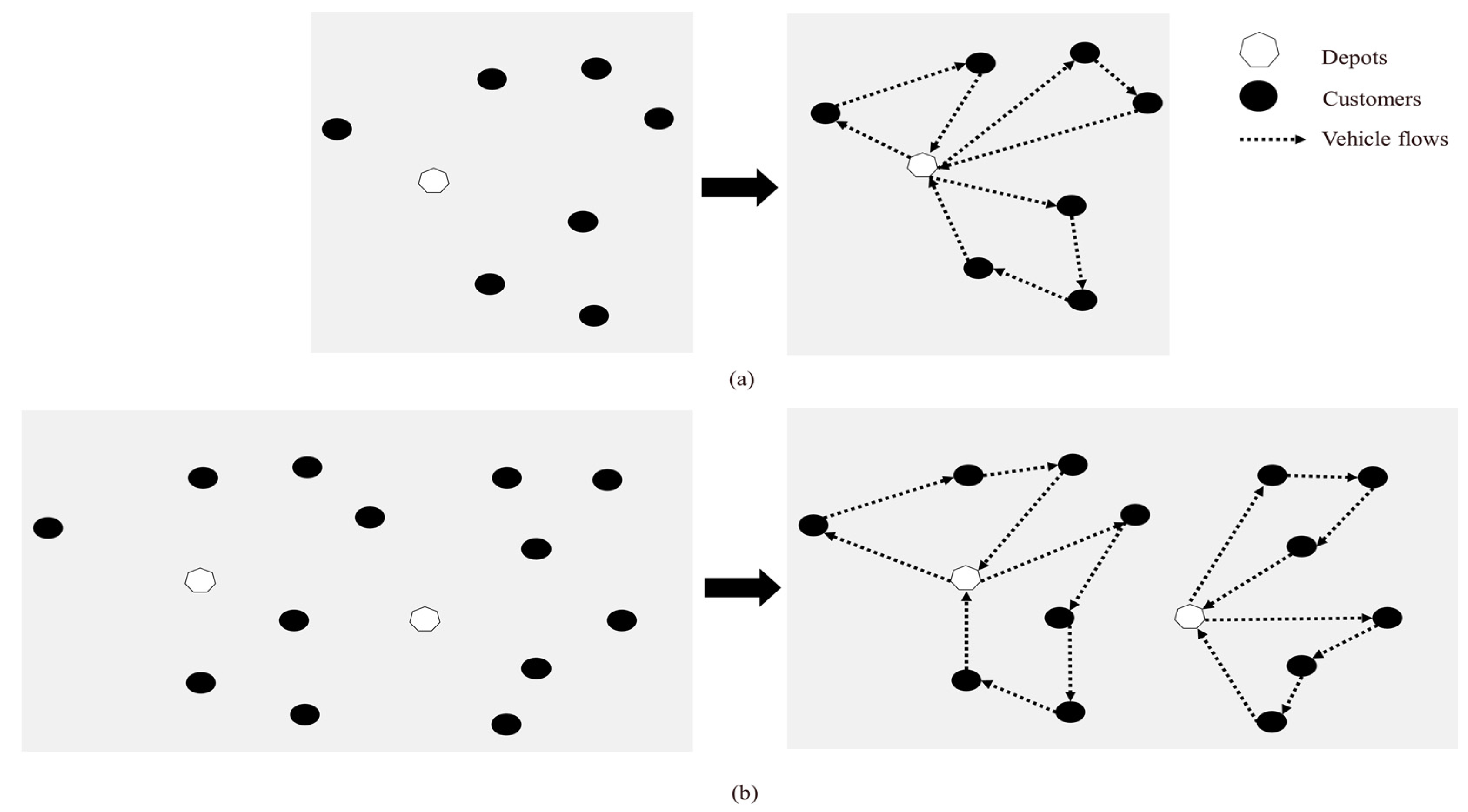
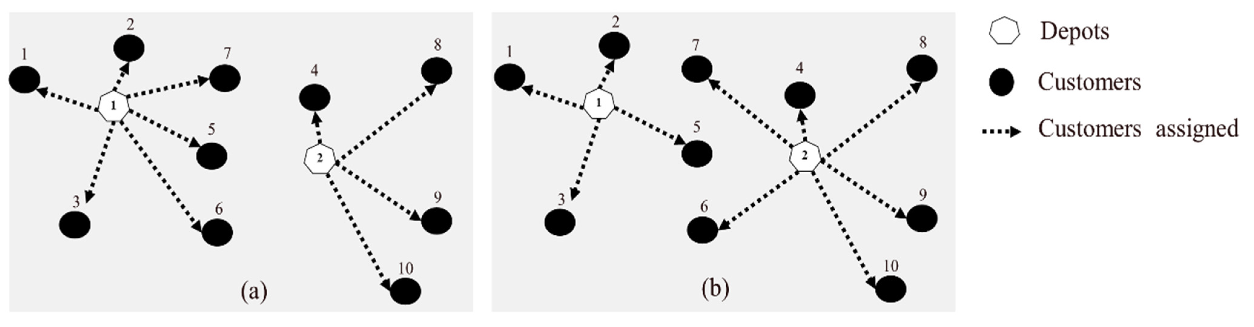
7]. Various egg products (e.g., egg powder) are produced, which are used in the food industry. Poultry distribution, regarding the design of the routing scheme for routing problems, is known as the multiple-depot vehicle-routing problem (MDVRP). One characteristic of this problem is that many customers need to be served by vehicles from many depots (e.g., egg distribution centers 1,2 and a slaughterhouse). Each vehicle must start at its depot, visit customers in order, and return to the same depot. Therefore, poultry distribution planning is intended to route the vehicle at each depot, with respect to the orders of customers.
The MDVRP has been the focus of many studies, as it is widely applicable to many real-world situations, including logistics distribution problems for optimizing total transportation costs. After all, an optimal route can minimize the total distance of each route, thereby leading to cost savings. Hence, it is essential to have an optimized plan for vehicle routing to complete poultry distribution.
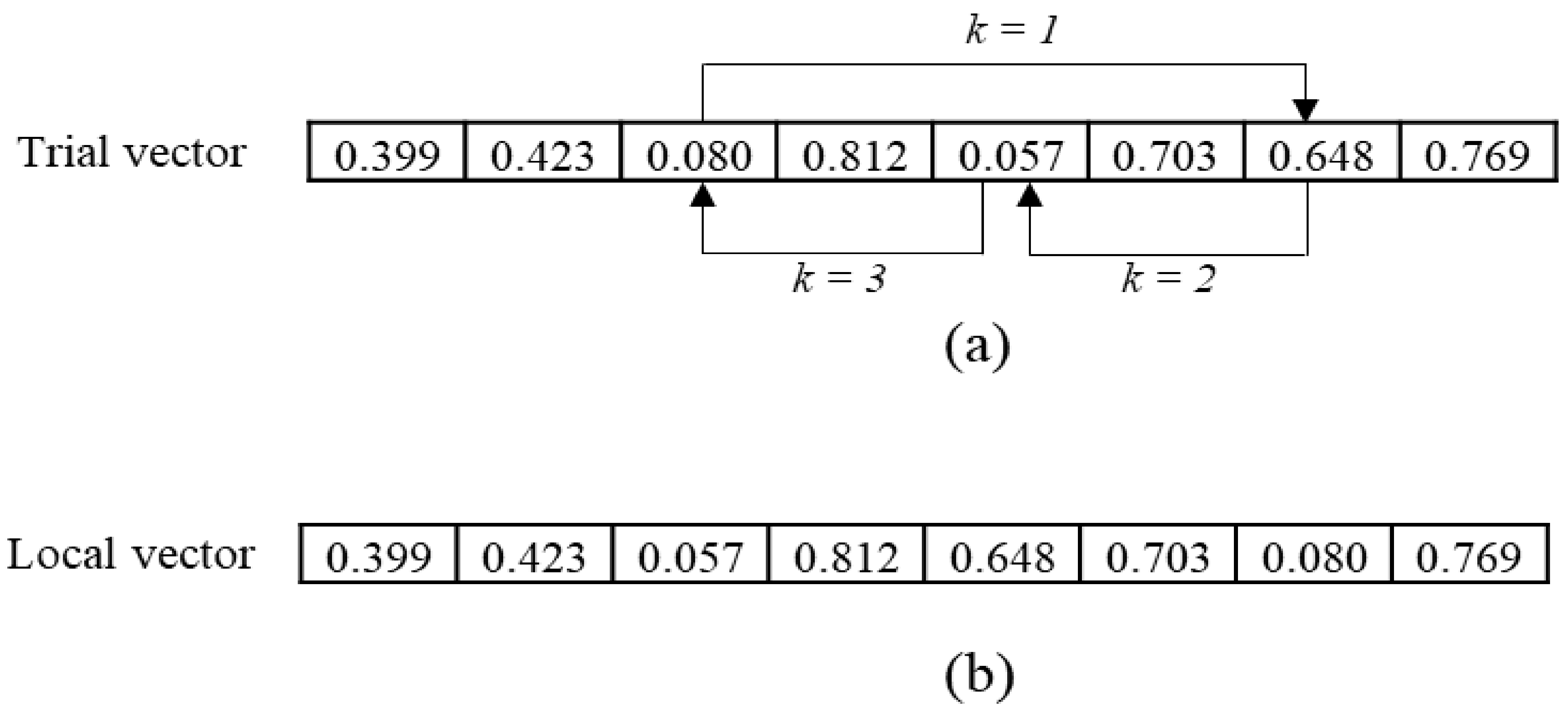
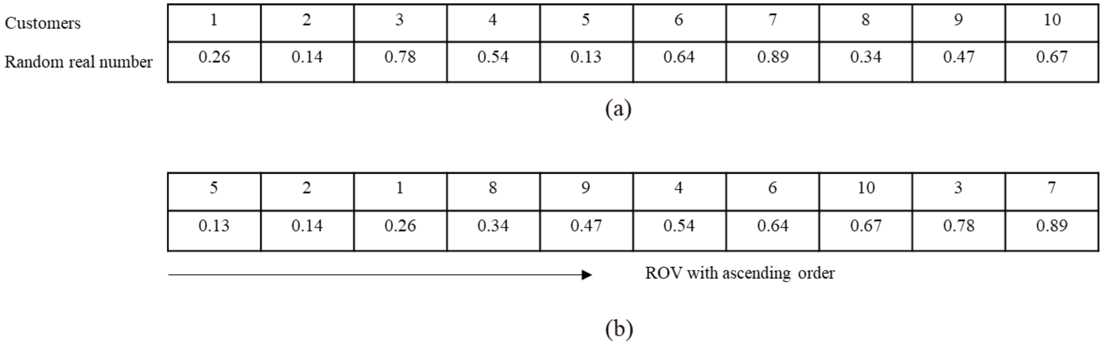
In this paper, we focus on outbound logistics planning of the poultry industry in Thailand, with the objective being to minimize transportation costs. We developed a mixed-integer linear programming (MILP) model for small-sized instances. In terms of large-sized instances, we developed a new enhanced differential evolution (DE) algorithm, which should make the best decision to minimize the distance between each depot and the customers. The main contributions of this paper are twofold. First, we developed a new mutation formula for re-initializing solutions for the DE algorithm in the context of protecting movements to a local optimal. Secondly, we designed an algorithm to further enhance the DE algorithm. The local search techniques were used in the k-variable move to improve the ability to search for the best solutions to enhance the exploitation search capability, called the local vector. Hence, using the re-initialization solution formula on the DE algorithm is known as the novel re-initialization solution and local search function on the DE algorithm (RI-DE), which will be implemented in Thailand’s Poultry Industry.
This paper is organized as follows: In Section 2, a review of the related literature is presented. Section 3 introduces the problem statement and formulation of MDVRP. Section 4 presents our proposed algorithm for solving the MDVRP. The computational results are discussed in Section 5. Finally, our conclusion is detailed in Section 6.

2. Literature Review

Developing an efficient production planning system for the poultry industry is challenging and interesting to manage, in terms of the supply chain and logistics; this is especially the case in the transportation planning for poultry, which is a process that covers activities involving both inbound, production, and outbound logistics. Optimizing operational and production planning results in lower operating costs and links to the outbound logistics system, where each customer receives the product according to their quantity demand. Therefore, this research aims to develop decision-making guidelines for solving poultry transportation planning problems based on obtaining globally optimal solutions, then developing a mathematical model for a mixed-integer linear program considering a single objective optimization problem to minimize the total cost of transportation, solving poultry transportation planning problems based on obtaining globally optimal solutions. By developing a mathematical model of a mixed-integer linear program considering a single objective optimization problem, the minimization of the total distance from each depot to all customers can be achieved.
The literature on open-innovation dynamics and multiple-depot vehicle-routing problems mainly considers three factors: MDVRP, metaheuristics in routing problems, and local search problems. In the following, we review the related papers in terms of these three directions.
Open innovation is intended for exploring and exploiting [8] new opportunities to obtain and develop new knowledge and technology [9], specifically in the poultry industry in Thailand, in which Small and Medium Enterprises (SMEs) assist in overcoming innovation obstacles [8,10,11]. In addition, previous research on open innovation investigates the importance of management in SMEs [12].
Given the novelty of open innovation dynamics in various research domains such as SMEs, as well as small and medium industries (SMIs), numerous studies have attempted to establish a precise description of this concept through research techniques by using qualitative methods such as system dynamics [13,14,15,16,17,18,19], theory-building [20,21,22] content analysis [3,23,24] optimization [12,25] and etc. Open innovation dynamics vary across different ecosystems [26], Moreover businesses’ attitudes toward open innovation result from a mix of the ecosystem’s various aspects [27,28].
Open innovation appears to be an ideal strategy for promoting a firm’s operations for knowledge exploration and exploitation to produce optimization software for routing problems in the context of Industry 4.0 technologies and their execution and integration [2,3]. Theeraviriga et al. [29] presented a new optimization technique for the location-routing problem of agriculture in Thailand. They developed a mathematical model and variable neighborhood strategy adaptive search (VaNSAS). They compared the solution of the proposed algorithm with the probability of selecting a black box in four different equations. Theeraviriga et al. [30] studied location decision making and transportation for the palm oil collection center. Firstly, they proposed a mixed-integer linear programming model (MILP) and adaptive large neighborhood search (ALNS). Then, the results were compared between the solution from the MILP by the LINGO program and ALNS. Supattananon and Akararungruangkul [31] presented a combination of a web application and the modified differential evolution (MDE) algorithm for the vehicle dispatching problem (VDP). They modified the DE with the probability of accepting the solution in the four different equations. The results demonstrated that the MDE outperformed the traditional DE.
Reviewing of the open innovation dynamics literature demonstrates that a combined approach of metaheuristic techniques such as genetic algorithm (GA), particle swarm optimization (PSO), and differential evolution (DE) algorithm in the field, planning the distribution of SMEs/SMIs, has not been used yet.
In 2015, Montoya-Torres et al. [32] provided a state-of-the-art survey on vehicle routing with multiple depots (MDVRP). Most of the initial papers on MDVRP considered transportation cost minimization. Moreover, due to the intricacy of transportation issues, there are numerous elements which should be as near to a real-world scenario as possible, including time windows, split delivery, heterogeneous fleets, periodic deliveries, and pickup and delivery.
Ho et al. (2008) [33] considered the topic of reverse logistics for a company that wants to collect cores from dealers during campaign seasons. Moreover, they proposed the distribution of products from multiple warehouses to sample customers in the transportation industry. This study developed two hybrid genetic algorithms (HGAs) to deal with the challenge efficiently. The primary distinction between the HGAs was that, in HGA1, the initial solutions were produced at random. For the initialization technique, HGA2 used the Clarke and Wright savings approach and the closest neighbor heuristic. Computational modeling was carried out in order to compare the methods with different issue sizes. In terms of overall delivery time, HGA2 outperformed HGA1. Aras, Aksen, and Tekin (2011) [34] presented two mixed-integer linear programming (MILP) models in MDVRP. They developed a Tabu search-based heuristic technique to modify medium- and large-sized cases, as the issue is NP-hard.
Sombuntham and Kachitvichyanukul (2010) [35] developed a particle swarm optimization algorithm with multiple social-learning structures (GLNPSO) to solve MDVRP with simultaneous pickup and delivery time windows. They created a new decoding technique, and their preliminary findings suggested that the proposed method could effectively solve most of the test issues.
Subsequently, many studies have focused on local search algorithms in MDVRP. A heuristic approach can tackle issues that are computationally difficult to solve. A local search may be employed to address issues when moving from one solution to the next in the context of candidate solutions, by making local adjustments until a solution which is deemed optimal is discovered, or a time limit has passed. Kuo and Wang (2012) [36] offered a variable neighborhood search (VNS) solution for the MDVRP with loading costs (LC). There were three phases in the proposed VNS: (1) Initial solution generation; (2) random neighborhood solutions; and (3) neighborhood solution acceptance by simulated annealing (SA). Their findings demonstrated that the proposed technique is both efficient and successful in addressing the related issues. In 2016, Alinaghian and Shokouhi [37] presented a hybrid algorithm composed of an adaptive large neighborhood search (ALNS) and VNS for a multi-compartment MDVRP. In the same year, Bezerra et al. [38] presented a modified randomized variable neighborhood descent (RVND) for solving MDVRP.
Sadati, Çatay, and Aksen (2021) [39] have recently developed a hybrid Tabu search and variable neighborhood search to escape from local optima; the algorithm was called the variable tabu neighborhood search (VTNS). The VTNS was used to solve three problems: MDVRP, MDVRPTW, and multi-depot open vehicle routing problem (MDOVRP). The study found that VTNS was competitive, in terms of the speed of solution, compared to state-of-the-art solution approaches published in the literature. Sethanan and Pitakaso (2016) [40] indicated a DE metaheuristic for the transportation of raw milk. In order to increase the quality of the solution, they developed five modified DE algorithms, including two new steps: reincarnation and survival processes. The modified DE algorithms offered higher efficiency in minimization of the total costs. Dechampai et al. (2015) [41] used the Multifactor Based Evolving Self-Organizing Maps with Differential Evolution for the General Q-Delivery Vehicle Routing Problem (G-Q-DVRP) with considerations of flexibility in mixing pickup and delivery services and the maximum duration of a route constraint (MESOMDE_G-Q-DVRP-FD) algorithm for the egg industry. The algorithm was beneficial for minimizing overall costs, compared to real-world cases, and for the efficient handling of a poultry production system.
Therefore, in the field of work related to the DE algorithm [40,41] we developed, in contrast to the above-mentioned works, the new mutation formula for re-initialization and new operation of using the k-valuable move algorithm in the DE algorithm.
Stodola (2018) [42] developed the ant colony optimization (ACO) theory to minimize the length of the longest route of all vehicles in the standard MDVRP. Later, Stodola (2020) [43] used a hybrid ant colony optimization algorithm. Mutual colony optimization was conducted twice. ACO applies the local optimization process, and updates pheromone trails according to selected solutions in a current generation, using the simulated annealing technique for decisions. The algorithm was found to minimize the total distance and the longest route for all vehicles. Zhang et al. (2020) [44] presented a multi-depot green vehicle routing problem considering alternative fuel-powered vehicles with limited fuel tank capacity. They proposed a two-stage ant colony system (TSACS). The proposed TSACS is distinguished through the utilization of two types of ants for two different objectives: the first type of ant was used to assign customers to depots, while the second type of ant was assigned to find the routes. The overall goal was to reduce total carbon emissions as much as possible. This approach could effectively reduce the total carbon emissions. Shi, Hu, and Han (2020) [45] considered waste collection problems from waste collection points to waste disposal plants formulated in terms of MDVRP. They presented the sector combination optimization (SCO) algorithm to generate initial solutions and used the merge-head and drop-tail (MHDT) strategy in the process of updating solutions to minimize the total transportation distance. This algorithm provided more effective solutions compared to the other algorithms presented, and used the lowest computational time in the tabu search to obtain near-optimal solutions. Zhen et al. [46] investigated a multi-depot multi-trip vehicle routing problem with time windows and release dates. They developed a mixed integer programming model for small-sized instances, and a hybrid particle swarm optimization algorithm and a hybrid genetic algorithm for large-sized instances. A summary of the past work on MDVRP is shown in Table 1.

3. Problem Statement and Mathematical Model

3.1. The Problem Statement

The logistic flow problem is also known as the vehicle routing problem (VRP). The VRP is an NP-hard combinatorial optimization problem that is designed to improve logistic planning to minimize the total cost. In this paper, we considered the outbound logistics for the poultry industry in Thailand. The outbound logistic in this case study is characteristic of multiple-depot vehicle routing problems. In summary, transportation from the depot to the customers must follow a circular route, with the depot serving as both a starting node and a destination node. When considering only one depot, the problem is known as a single-depot problem, or VRP (see Figure 2a). Meanwhile, when the number of depots increases, it is known as the multi-depot vehicle problem (see Figure 2b). The objective of this paper is to find the best plan for the poultry industry that minimizes transportation costs.

3.2. The Mathematical Model

This paper used the mixed-integer linear programming of MDVRP based on the first presented by Kulkarni and Bhave [47]. The mathematical model of the MDVRP defines a three-index binary decision, where the binary decision variable x i j k is equal to 1 when linking the arc between customers i and j in the route of vehicle k, and 0 otherwise. We consider assumptions that are used in the poultry distribution industry based on MDVRP:
(1)
Each vehicle must depart from and return to the same depot;
(2)
Each customer is served exactly once by one vehicle;
(3)
The customer’s demand does not exceed the vehicle capacity;
(4)
All customers needs are met; and
(5)
The total time of a route does not exceed the maximum duration time of the route.
The following notation is used in the model:
Sets and indices:
M Set of poultry distribution center (depot) nodes
N Set of customer nodes
K Set of vehicles
i , j Index of nodes;   i , j = 1 , , N + M
k Index of vehicles;   k = 1 , , K
Parameters:
c i j Transportation cost between customers i and j
t i j Transportation time between customers i and j
Q i Demand at customer i
P k Capacity of vehicle k
T k Maximum duration time of route allowed for vehicle k
Decision variables:
x i j k Equal to 1 if the vehicle k is traveling from customer i to customer j, zero otherwise
u i An integer variable that defines the order of vertices visited on a tour for the elimination of sub-tours
The formulation of poultry distribution based on MDVRP can be stated as follows:
M i n i m i z e   Z = i = 1 N + M j = 1 N + M k = 1 K c i j x i j k
Subject to:
i = 1 N + M k = 1 K x i j k = 1                   j = 1 , , N  
j = 1 N + M k = 1 K x i j k = 1               i = 1 , , N  
i = 1 N + M x i h k j = 1 N + M x h j k = 0               k = 1 , , K h = 1 , , N + M
i = 1 N + M j = 1 N + M Q i x i j k P k                   k = 1 , , K
i = 1 N + M j = 1 N + M t i j x i j k T k           k = 1 , , K  
i = N + 1 N + M j = 1 N x i j k 1               k = 1 , , K
j = N + 1 N + M i = 1 N x i j k 1               k = 1 , , K
u i u j + N + M x i j k N + M 1           1 i j N   a n d   1 k K
x i j k ϵ   0 , 1                     k = 1 , , K i , j = 1 , , N + M
u i 0                                   i = 1 , , N + M
The objective function (1) of the poultry industry distribution is to minimize the transportation cost. Constraints (2) and (3) denote a single visit, and that a single vehicle serves the customer. Constraints (4) states that any vehicle that visits a customer should also depart from that customer. Constraints (5) ensure that the demand at customer i ( Q i ) cannot exceed its vehicle capacity ( P k ). Constraint (6) ensures that a vehicle k is returned to the depot no later than the maximum duration time ( T k ) . Vehicle availability is verified by constraints (7) and (8). Constraint (9) is for sub-tour elimination. Finally, constraint (10) and (11) serves as the basis for the decision variables.

4. New Enhanced Differential Evolution Algorithms

The differential evolution (DE) algorithm is a population-based search, which was proposed by Storn and Price [48]. The DE algorithm includes three operations: Mutation, recombination, and selection. The vector containing dimension (D) variables is denoted by x i , j t . The pseudocode of the traditional DE algorithm is shown in Algorithm 1. This section presents a new, enhanced DE algorithm with a new mutation formula to adapt between the mutation formula DE / rand / 1 and the local mutation vector and local search function. The proposed algorithm is named RI-DE, and its steps are shown in Algorithm 2. The details of the procedures are as follows.
Algorithm 1 The pseudocode of DE
1.Define the objectives function f(x)
2.Generate the initial population of NP
3.while t < Max(number of iteration)
4.for each     x i t in the population do
5. Random   vector   r 1 , r 2 , r 3   (1,NP), with r1r2r3
6. Generete   a   random   integer   j rand (1, D)
7.  for each parameter j do
8.     Generate   v i t through Equation (12)
9.     Generate   u i   t through Equation (13)
10.  end for
11. Replace     x i t   with   the   u i   t   if   u i   t is better through Equation (16)
12.end for
13.end while

4.1. Initialization Operation

The initial individuals vector   x i , j 0 (i = 1,…,NP) generates random numbers within the range [0, 1), and the maximum number of iterations tmax for the current generation t is set as 0 (note: For understanding   x i t is a target vector i iteration t does not reference dimension j, which   x i , j t references dimension j, that the same variable).

4.1.1. New Mutation Operation

For each   x i t in the population, the mutant vector v i t + 1 is generated by the mutation formula. The traditional DE uses the following mutation formula:
DE / rand / 1   :   v i t + 1 =   x r 1 t + F   x r 2 t x r 3 t ,
where r1, r2, and r3 form a random vector chosen within the range [1,NP], and each r must be different (i.e., r1 ≠ r2 ≠ r3). F is the is the scaling factor. The new enhanced DE is developed considering the following mutation operation.
The new mutation operation was developed considering the concept of protecting the moving trap solution, as the search performance of DE still needs to be improved. The mutant vector, v i t + 1 , is generated by the mutation formula as follows:
v i t + 1 = x r n e w t + F   x b e s t t x i t   + F   x r 1 t x r 2 t ,         i f   N I R I             x r 1 t + F   x r 2 t x r 3 t ,       o t h e r w i s e                                                                                                
where x r n e w t   , x b e s t t   ,   N I ,   and   R I   are the new random vector, the vector that obtains the best solution at iteration t (called the best vector), the number of iterations after which the solution does not improve, and the number of cumulative iterations in which the solution does not improve (function re-initialization is used), respectively. Moreover, the percentage of the number of populations P s for random populations used Equation (13). We set the parameter P s equal to 20% based on previous work [49]. We hope to use a new mutation formula to protect against trapping in local optima.

4.1.2. The Recombination Operation

For this study, we adopted the binominal recombination operation. For each target vector   x i , j 0 , the trial vector u i , j   t   was generated as follows:
u i , j   t + 1 =     v i , j t + 1 ,     i f   r j C R   o r   j = r a n d n i x i , j t   ,     o t h e r w i s e ,                                                                      
where rj, j, and CR are a random number within the range [0, 1], a random integer within the number of dimensions D, and the crossover probability within the range [0, 1], respectively.
Algorithm 2: The pseudocode of RI-DE
1.Define the objectives function f(x)
2.Generate the initial population of NP
3.while t < Max(number of iteration)
4.for each   x i t in the population do
5. Random   vector   r 1 ,   r 2 ,   r 3   (1,NP), with r1r2r3
6. Generete   a   random   integer   j rand   (1, D)
7.  for each parameter j do
8.   if N I R I
9.     Generate   v i t through Equation (12)
10.   else
11.    if   Random   each     x i t in population with Ps%
12.       Generate   v i t through Equation (13)
13.       Generate   u i   t through Equation (14)
14.    else
15.      Generate   v i t through Equation (12)
16.       Generate   u i   t through Equation (14)
17.    end
18.   end
19.   Call local search function
20.   Generate l i   t through local search function
21.     Replace   u i t   with   the   l i   t   if   l i   t   is   better ,   and   u i   t otherwise through Equation (15)
22.  end for
23. Replace     x i t   with   the   u i t   if   u i t is better through Equation (16)
24.end for
25.end while

4.1.3. The Local Search Functions

The RI-DE algorithm used a local search algorithm (e.g., swap function, insert function, and 2-opt function), in order to improve the exploitation ability of the search in the context of protecting movements to a local optimum. To create a new vector, the local search function (called the local vector, l i t ) from Equation (15), is operated in each dimension j by the local search function to create the l i , j t . The new trial vectors u i , j t are selected as follows:
u i , j t = l i , j t   ,     i f     f l i , j t   f u i , j t             u i , j   t ,                     o t h e r w i s e                                              
Our proposed algorithm uses a local search name k-variable move algorithm [50]. The k-variable move is an extended version of the swap algorithm, in which k continues to move from a k position to the next k position until the last k moves to the first k in D.
For example, after the trial vector u i , j   t is created (see Figure 3), a k-variable move (where k = 3) is shown in Figure 3. The trial vector is randomized in three positions {3,7,5} (see Figure 3a), swapping from the first position to the next position. Finally, the third position must move to the first position (see Figure 3b).
In this paper, we used k = 20% based on previous work [49], which means that k should be the random number for moving up to around 20% of the customers.

4.1.4. Selection Operation

If the fitness value of the trial vector is better than the target vector, then the trial vector replaces the target vector with a pre-target vector in the next iteration based on a greedy selection.
x i , j   t + 1 = u i , j t   ,     i f     f u i , j t   f x i , j t   x i , j t   , o t h e r w i s e  
In the brief discussion of Algorithm 1, each individual of the trial vector is compared to the objective function with its target vector, and the better one is selected for the next iteration. Then, these steps are repeated until the stopping criterion is reached. Moreover, the critical difference between Algorithms 1 and 2 is that in Algorithm 2, when the solution does not develop, Equation (13) is used, the individual target vector is random with PS% chance to be the local vector, and the better one between the trial vector and local vector is chosen to be new trial vector that is compared with its target vector.

4.2. The Decoding Method

The solution to our proposed problem is the use of multiple vehicle routes for the poultry distribution problem to deliver products from the multi-depot to customers within the limited number of vehicles at each depot. The following example shows the decoding method: suppose we have two depots. Then, the limited number of vehicles at each depot is two, the vehicle capacity in a homogeneous fleet is equal to 40, and there are 10 customers. The demand of the 10 customers is shown in Table 2.
In our proposed algorithm, the dimension in the vector represents the solutions. In the first array, each dimension is identified by a customer sequence, which is sorted by increasing values. In the second array, each dimension is identified by a corresponding random real-number sequence (see Figure 4a). Therefore, the customer sequence of each depot can be obtained by rank order value (ROV), which decodes the ascending order (see Figure 4b).

4.2.1. The Customer Assigned

The customer assigned to each depot is chosen based on the greedy algorithm. The customers must select a closer depot for delivering products for them. The objective of this paper is to minimize the overall transportation costs. Thus, the customers are assigned to the nearest depots. For example, each of the 10 customers should be assigned to nearby depots, as shown in Table 2, column 3.

4.2.2. Solution Representation of RI-DE Algorithm

Each vector is structured as a double array, with the length being the number of customers in this algorithm (|N|). Figure 4 depicts an example of the decoding method of RI-DE, where |N| equals 10. The vector with random positioning of customers is shown in Figure 4a. The customers in {1, 3, 6, 8, 10} are assigned to depot 1. Similarly, customers in {2, 4, 5, 7, 9} are assigned to depot 2. Therefore, the customer sequences are depicted as {5, 2, 1, 8, 9, 4, 6, 10, 3, 7} (see Figure 4b), in which the customer sequences of depot 1 and depot 2 are {1, 8, 6, 10, 3} and {5, 2, 9, 4, 7}, respectively. The routing of vehicles for each customer is available with respect to the vehicle capacity and the maximum number of vehicles at each depot.
(1)
Route No. 1: Vehicle No. 1 at Depot 1. The routing assignment: The vehicle has to deliver products to customers {1,8,6} with amounts of 10, 16, and 10, respectively, as the products loaded are inadequate to meet the demand of the following customers: customer number 10 had a demand of 14, but there were only four remaining products (40–10−16–10 = 4). Hence, the vehicle must then return to Depot 1.
(2)
Route No. 2: Vehicle No. 2 at Depot 1. This is similar to Route No. 1 at Depot 1, but Vehicle No. 2 has to deliver to the remaining customers ({10,3}).
(3)
Route No. 3: Vehicle No. 3 at Depot 2. The routing assignment: The vehicle has to deliver products to customers {5, 2, 9} with amounts of 18, 12 and 10, respectively; however, the products loaded were not enough to meet the demand of the following customers: customer number 4 had a demand of 15, but there were no remaining products (40–18−12–10 = 0). The vehicle must return to Depot 2.
(4)
Route No. 4: Vehicle No. 4 at Depot 2. This is similar to Route No. 3 Vehicle No. 3 at Depot 2., but Vehicle No. 2 at Depot 2 has to deliver to the remaining customers ({4, 7}).
Suppose the number of vehicles in service is insufficient to meet the demands of the customers. In that case, it is necessary to move the number of customers that cannot be served to the next nearest depot. For example, customers {5,3,2,1,6,7} are assigned to be serviced by depot 1 (see Figure 5a), while customers {4,8,9,10} must be serviced by depot 2. It is found that the number of vehicles at depot 1 can only serve customers {5,3,2,1}, while customers {6,7} cannot be serviced as the number of vehicles at depot 1 are inadequate. Thus, it is necessary to assign customers {6,7} to the next nearest depot to receive service. Suppose the next nearest depot is depot 2, where the sequence will be appended to the original order, becoming {4,8,9,10,6,7} (see Figure 5b).

5. Computational Experiment

In this section, the experiments were executed on a computer with the following parameters: Intel® Core™ i7-8750H CPU @ 2.20 GHz, 2.21 GHz RAM, and 16.0 GB. We developed the mathematical model in LINGO software, based on the branch and bound method, and our proposed algorithms were coded in MATLAB (R2018a). The implementation of our proposed algorithm requires parameters, as provided in Table 3 [7,51,52,53]. We divided the parameters into small- and large-sized instances, shown in the third and fourth columns, respectively. For each experimental set, we attempted 15 replicates. Comparisons based on several population-based algorithms were discovered as well, such as traditional differential evolution (DE) algorithm, genetic algorithm (GA) [54,55], and particle swarm optimization (PSO) [55].
The results of our proposed algorithms were compared with LINGO for small-sized instances, as illustrated in Table 4, which is organized as follows. The first column contains the number of the instance ID. Column 2 contains the instance ID. In addition, each instance comprises three parts: the number of depots, the number of customers, and the number of vehicles. In column three, we show the optimal solution obtained by LINGO. Columns 4–12 show the best, average, and worst solutions obtained by the genetic algorithm (GA), particle swarm optimization (PSO), traditional differential evolution (DE), and re-initialization differential evolution (RI-DE) algorithm. We tested a total of 25 instances with 5, 10, 15, 20, and 25 customers. The number of the depots was 2, 3, and 4 depots. The numbers of vehicles at each depot were 3, 4, 5, and 6 vehicles. We used the best solution obtained from the 15 replicates of our proposed algorithm to demonstrate the transportation cost. The computational time of our proposed algorithms is shown in Table 5.
The case study (CS) on this research was motivated by the small and medium-sized enterprises (SMEs) in northeastern Thailand. Currently, the total number of distribution centers is 6 with customers numbering about 500. To deliver to the customers, the case-study company has a contract with a third-party delivery company, which provides about 250 vehicles.
In Table 6, the heuristic performance (HP) percentage is shown, which was calculated as HP = (SL/So) × 100. Here, SL and So are the solutions obtained by LINGO and the solution obtained by our proposed algorithm in Table 4, respectively. The statistical test results in the solution obtained by our proposed algorithm using the Wilcoxon test are shown in Table 7. We used the Wilcoxon test because it neither depends on the form of the parent distribution nor its parameters and does not depend on any assumptions about the shape of the distribution or on being normally distributed. The statistical test was performed based on the transportation cost of LINGO and our proposed algorithm, and the SPSS V14 software for Windows was used to carry out the statistical analysis.
Our proposed algorithm could also obtain the optimal solutions for instances 1 to 10 from Table 4 (see bold numbers in Table 4). However, for instances 11 to 25, our proposed algorithm found near-optimal solutions. The best solutions for our proposed algorithms were 12/15, 2/15, 1/15, and 0/15 times by RI-DE, DE, PSO, and GA, respectively, which implies the new formula of the re-initialization DE algorithm and the local search function can improve protection against trapping in local optima for small-sized instances. The average computational time of the mathematical model (LINGO) and our proposed algorithms were 9922.40, 2.98, 3.01, 3.16, and 4.95 s with LINGO, GA, PSO, DE, and RI-DE, respectively.
The statistical test results demonstrated that the RI-DE algorithm obtained solutions that differed in a statistically significant manner from the other algorithms (p-value ≤ 0.05). In addition, in our experiments, we found that the DE and PSO did not significantly differ. In terms of small-sized instances, RI-DE outperformed the other proposed algorithms.
In large-sized instances, where LINGO cannot obtain solutions, our proposed algorithm was evaluated on Cordeau’s benchmark instances. The best knowledge solutions were taken from NEO Web, with all instances available for download at https://neo.lcc.uma.es/vrp/vrp-instances (23 September 2021).
Table 8 shows some properties of Cordeau’s benchmark instances for each instance; the numbers of nodes (N) and depots (M) are shown, as well as the results of the GA, PSO, traditional DE and RI-DE algorithms, in terms of the best and average solutions found. Our proposed algorithm ran 10 replicates on all instances. The best solutions, average solutions, and average computational time of our proposed algorithm are recorded. The numbers in bold in the best solutions columns record the best-known solutions (BKS) taken from our proposed algorithm.
The results for the 23 instances of Cordeau’s benchmark in Table 9 report the deviation from the best-known solutions (Δ) for our proposed algorithms. The last column reports the percentage relative improvement (RI%) between the traditional DE and RI-DE algorithm, calculated by RI = (SDE − SRI-DE/SDE) × 100. Here, SDE and SRI-DE are the solutions obtained by the traditional DE and RI-DE algorithms, respectively. The average deviation from the best-known solutions (Δ) for different GA, PSO, DE and RI-DE algorithms was 9.98%, 6.15%, 4.05% and 1.48%, respectively. In addition, the average percentage of relative improvement between the traditional DE and RI-DE algorithms was 2.53%. Also, when considering the large-sized instances from Cordeau’s benchmark, it was demonstrated that the RI-DE algorithm outperforms the traditional DE algorithm.
The discussion of metaheuristics and open innovation is applied to the features of outbound logistics for distribution in order to develop the new optimized technique. in our opinion, the metaheuristic can be applied to minimize the transportation of the poultry industry in Thailand. One of the complexities of multiple vehicle routing problems is the NP-hard problem [47]. However, many researchers have considered the problem of open innovation [29,30,31]. To develop the optimization software for finding the optimal solution for the vehicle routing problem, it is discussed how the open innovation concept can be applied to the metaheuristics technique, such as our proposed algorithm to industrial dynamics perspective. Moreover, this paper is virtually the first case in which the differential evolution algorithm has been enhanced using the re-initialization mutation formula and local search function, in terms of the theoretical implications of open innovation among the poultry industry SMEs in Thailand via the concept of open innovation [1].
As a result, it is essential to remember that it extends beyond traditional logistical boundaries. A concept model of open innovation developed in [26] aims to investigate current open innovation channels, which might motivate engineering research to increase open innovation and the creation of new open-business models from meta-heuristics.

6. Conclusions

This paper focused on the planning of outbound logistics for the poultry industry in Thailand. The problem involves the planning of distribution of poultry products where the distribution center has more than one depot, making the situation characteristic of the multi-depot vehicle routing problem (MDVRP), which aims to minimize transportation costs.
Considering the NP-Hardness of our proposed problem, a new enhanced DE algorithm composed of a re-initialization solution and a local search function was developed. In the computational results, our proposed algorithm reached the optimal solution in small-sized instances (numbers 1–10). The average transportation costs of our proposed algorithm for small-sized instances for LINGO (exact method), GA, PSO, DE, and RI-DE were equal to 10,245.64, 10,727.49, 10,518.37, 10,465.73, and 10,379.83, respectively. The average computational times for LINGO (exact method), GA, PSO, DE, and RI-DE were equal to 9922.40, 2.98, 3.01, 3.16, and 4.95 s, respectively. The statistical test showed that the RI-DE solution obtained based on transportation costs was significantly different from the solutions from the GA, PSO, and DE algorithms. Heuristic performance (HP) indicated that GA, PSO, DE, and RI-DE obtained near-optimal results, with an average of 96.48, 97.97, 98.33 and 99.03% respectively. The experimental results showed that the IR-DE algorithm obtained a near-optimal solution ranging from 96.62% to 100% of 15 replicated runs. When solving large-sized instances on Cordeau’s benchmark instances, the enhanced DE algorithm (RI-DE) returned 1.48% error on average, which was significantly lower than that of the traditional DE algorithm. Moreover, given that the relative improvement (RI) comparing the transportation cost obtained from the traditional DE to that of RI-DE was equal to 2.53% on average, the results show that the RI-DE algorithm provides better transportation cost that the DE algorithm, ranging from 0.00% to 9.68%.
The RI-DE algorithm demonstrated an ability to obtain effective solutions by using the re-initialization mutation formula and local search function. The re-initialization solution could protect against trapping in local optima when the solution did not improve and create new vectors to find the best solution. In addition, the local search function was used to enhance the exploitation searchability of the DE algorithm. This implies that the re-initialization mutation formula and the local search function significantly improved the DE algorithm.
Future work can be extended in the following directions: firstly, there is still much opportunity to extend our work in many aspects when there are multiple periods, multiple products, heterogeneous fleets, and time window constraints, which may also provide an interesting topic for minimizing the total cost, including transportation, holding, and hiring costs. Secondly, the performance of the algorithm will be assessed in other real-world environments involving difficult combinatorial optimization problems in logistics and supply management. Lastly, our proposed algorithm could be extended to solve problems in other industries, i.e., agriculture and food.

Author Contributions

Conceptualization, K.M. and K.S.; methodology, K.M.; software, K.M.; validation, K.M. and K.W.; formal analysis, K.M.; data curation, K.M.; writing—original draft preparation, K.M.; writing—review and editing, K.M., K.S. and K.W.; supervision, K.M. and K.S.; project administration, K.S. All authors have read and agreed to the published version of the manuscript.

Funding

This research received Faculty of Engineering, Khon Kaen University, Thailand.

Institutional Review Board Statement

Not applicable.

Informed Consent Statement

Not applicable.

Data Availability Statement

Data sharing not applicable.

Acknowledgments

This work is supported by the Research Unit on System Modeling for Industry, Department of Industrial Engineering, Faculty of Engineering, Khon Kaen University, Thailand.

Conflicts of Interest

The authors declare no conflict of interest.

References

  1. Sengupta, A.; Sena, V. Impact of Open Innovation on Industries and Firms—A Dynamic Complex Systems View. Technol. Forecast. Soc. Chang. 2020, 159, 120199. [Google Scholar] [CrossRef]
  2. Shcherbakov, V.; Silkina, G. Supply Chain Management Open Innovation: Virtual Integration in the Network Logistics System. J. Open Innov. Technol. Mark. Complex. 2021, 7, 54. [Google Scholar] [CrossRef]
  3. Mubarak, M.F.; Petraite, M. Industry 4.0 Technologies, Digital Trust and Technological Orientation: What Matters in Open Innovation? Technol. Forecast. Soc. Chang. 2020, 161, 120332. [Google Scholar] [CrossRef]
  4. Woschank, M.; Dallasega, P. The Impact of Logistics 4.0 on Performance in Manufacturing Companies: A Pilot Study. Procedia Manuf. 2021, 55, 487–491. [Google Scholar] [CrossRef]
  5. Barykin, S.Y.; Kapustina, I.V.; Sergeev, S.M.; Yadykin, V.K. Algorithmic Foundations of Economic and Mathematical Modeling of Network Logistics Processes. J. Open Innov. Technol. Mark. Complex. 2020, 6, 189. [Google Scholar] [CrossRef]
  6. Boonmee, A.; Sethanan, K.; Arnonkijpanich, B.; Theerakulpisut, S. Minimizing the Total Cost of Hen Allocation to Poultry Farms Using Hybrid Growing Neural Gas Approach. Comput. Electron. Agric. 2015, 110, 27–35. [Google Scholar] [CrossRef]
  7. Boonmee, A.; Sethanan, K. A GLNPSO for Multi-Level Capacitated Lot-Sizing and Scheduling Problem in the Poultry Industry. Eur. J. Oper. Res. 2016, 250, 652–665. [Google Scholar] [CrossRef]
  8. Keupp, M.M.; Gassmann, O. Determinants and Archetype Users of Open Innovation. R D Manag. 2009, 39, 331–341. [Google Scholar] [CrossRef]
  9. Han, J.; Heshmati, A. Determinants of Financial Rewards from Industry-University Collaboration in South Korea. Int. J. Entrep. Innov. Manag. 2016, 20, 235–257. [Google Scholar] [CrossRef]
  10. Heikkilä, M.; Bouwman, H.; Heikkilä, J. From Strategic Goals to Business Model Innovation Paths: An Exploratory Study. J. Small Bus. Enterp. Dev. 2018, 25, 107–128. [Google Scholar] [CrossRef] [Green Version]
  11. Radicic, D.; Djalilov, K. The Impact of Technological and Non-Technological Innovations on Export Intensity in SMEs. J. Small Bus. Enterp. Dev. 2019, 26, 612–638. [Google Scholar] [CrossRef]
  12. Hakaki, A.; Shafiei Nikabadi, M.; Heidarloo, M.A. An Optimized Model for Open Innovation Success in Manufacturing SMES. RAIRO-Oper. Res. 2021, 55, 3339–3357. [Google Scholar] [CrossRef]
  13. Amrina, U.; Hidayatno, A.; Zagloel, T.Y.M. A Model-Based Strategy for Developing Sustainable Cosmetics Small and Medium Industries with System Dynamics. J. Open Innov. Technol. Mark. Complex. 2021, 7, 225. [Google Scholar] [CrossRef]
  14. Yuana, R.; Prasetio, E.A.; Syarief, R.; Arkeman, Y.; Suroso, A.I. System Dynamic and Simulation of Business Model Innovation in Digital Companies: An Open Innovation Approach. J. Open Innov. Technol. Mark. Complex. 2021, 7, 219. [Google Scholar] [CrossRef]
  15. Peñarroya-Farell, M.; Miralles, F. Business Model Dynamics from Interaction with Open Innovation. J. Open Innov. Technol. Mark. Complex. 2021, 7, 81. [Google Scholar] [CrossRef]
  16. Skordoulis, M.; Ntanos, S.; Kyriakopoulos, G.L.; Arabatzis, G.; Galatsidas, S.; Chalikias, M. Environmental Innovation, Open Innovation Dynamics and Competitive Advantage of Medium and Large-Sized Firms. J. Open Innov. Technol. Mark. Complex. 2020, 6, 195. [Google Scholar] [CrossRef]
  17. Lee, M.H.; Yun, J.H.J.; Pyka, A.; Won, D.K.; Kodama, F.; Schiuma, G.; Park, H.S.; Jeon, J.; Park, K.B.; Jung, K.H.; et al. How to Respond to the Fourth Industrial Revolution, or the Second Information Technology Revolution? Dynamic New Combinations between Technology, Market, and Society through Open Innovation. J. Open Innov. Technol. Mark. Complex. 2018, 4, 21. [Google Scholar] [CrossRef] [Green Version]
  18. Yun, J.J.; Park, K.B.; Hahm, S.D.; Kim, D. Basic Income with High Open Innovation Dynamics: The Way to the Entrepreneurial State. J. Open Innov. Technol. Mark. Complex. 2019, 5, 41. [Google Scholar] [CrossRef] [Green Version]
  19. Casquejo, M.N.; Himang, C.; Ocampo, L.; Ancheta, R.; Himang, M.; Bongo, M. The Way of Expanding Technology Acceptance-Open Innovation Dynamics. J. Open Innov. Technol. Mark. Complex. 2020, 6, 8. [Google Scholar] [CrossRef] [Green Version]
  20. Barrett, G.; Dooley, L.; Bogue, J. Open Innovation within High-Tech SMEs: A Study of the Entrepreneurial Founder’s Influence on Open Innovation Practices. Technovation 2021, 103, 102232. [Google Scholar] [CrossRef]
  21. Dahlander, L.; Gann, D.M.; Wallin, M.W. How Open Is Innovation? A Retrospective and Ideas Forward. Res. Policy 2021, 50, 104218. [Google Scholar] [CrossRef]
  22. Almeida, F. Open-Innovation Practices: Diversity in Portuguese Smes. J. Open Innov. Technol. Mark. Complex. 2021, 7, 169. [Google Scholar] [CrossRef]
  23. Iqbal, M.; Suzianti, A. New Product Development Process Design for Small and Medium Enterprises: A Systematic Literature Review from the Perspective of Open Innovation. J. Open Innov. Technol. Mark. Complex. 2021, 7, 153. [Google Scholar] [CrossRef]
  24. Baierle, I.C.; Siluk, J.C.M.; Gerhardt, V.J.; Michelin, C.D.F.; Junior, Á.L.N.; Nara, E.O.B. Worldwide Innovation and Technology Environments: Research and Future Trends Involving Open Innovation. J. Open Innov. Technol. Mark. Complex. 2021, 7, 229. [Google Scholar] [CrossRef]
  25. Shmatko, A.; Barykin, S.; Sergeev, S.; Thirakulwanich, A. Modeling a Logistics Hub Using the Digital Footprint Method—The Implication for Open Innovation Engineering. J. Open Innov. Technol. Mark. Complex. 2021, 7, 59. [Google Scholar] [CrossRef]
  26. Yun, J.H.J.; Zhao, X.; Jung, K.H.; Yigitcanlar, T. The Culture for Open Innovation Dynamics. Sustainability 2020, 12, 5076. [Google Scholar] [CrossRef]
  27. Lyu, Y.; He, B.; Zhu, Y.; Li, L. Network Embeddedness and Inbound Open Innovation Practice: The Moderating Role of Technology Cluster. Technol. Forecast. Soc. Chang. 2019, 144, 12–24. [Google Scholar] [CrossRef]
  28. Radziwon, A.; Bogers, M. Open Innovation in SMEs: Exploring Inter-Organizational Relationships in an Ecosystem. Technol. Forecast. Soc. Chang. 2019, 146, 573–587. [Google Scholar] [CrossRef]
  29. Theeraviriya, C.; Pitakaso, R.; Sethanan, K.; Kaewman, S.; Kosacka-Olejnik, M. A New Optimization Technique for the Location and Routing Management in Agricultural Logistics. J. Open Innov. Technol. Mark. Complex. 2020, 6, 11. [Google Scholar] [CrossRef] [Green Version]
  30. Theeraviriya, C.; Pitakaso, R.; Sillapasa, K.; Kaewman, S. Location Decision Making and Transportation Route Planning Considering Fuel Consumption. J. Open Innov. Technol. Mark. Complex. 2019, 5, 27. [Google Scholar] [CrossRef] [Green Version]
  31. Supattananon, N.; Akararungruangkul, R. Modified Differential Evolution Algorithm for a Transportation Software Application. J. Open Innov. Technol. Mark. Complex. 2019, 5, 84. [Google Scholar] [CrossRef] [Green Version]
  32. Montoya-Torres, J.R.; Franco, J.L.; Isaza, S.N.; Jiménez, H.F.; Herazo-Padilla, N. A Literature Review on the Vehicle Routing Problem with Multiple Depots. Comput. Ind. Eng. 2015, 79, 115–129. [Google Scholar] [CrossRef]
  33. Ho, W.; Ho, G.T.S.; Ji, P.; Lau, H.C.W. A Hybrid Genetic Algorithm for the Multi-Depot Vehicle Routing Problem. Eng. Appl. Artif. Intell. 2008, 21, 548–557. [Google Scholar] [CrossRef]
  34. Aras, N.; Aksen, D.; Tuǧrul Tekin, M. Selective Multi-Depot Vehicle Routing Problem with Pricing. Transp. Res. Part C Emerg. Technol. 2011, 19, 866–884. [Google Scholar] [CrossRef]
  35. Sombuntham, P.; Kachitvichyanukul, V. Multi-Depot Vehicle Routing Problem with Pickup and Delivery Requests. AIP Conf. Proc. 2010, 1285, 71–85. [Google Scholar] [CrossRef] [Green Version]
  36. Kuo, Y.; Wang, C.-C. A Variable Neighborhood Search for the Multi-Depot Vehicle Routing Problem with Loading Cost. Expert Syst. Appl. 2012, 39, 6949–6954. [Google Scholar] [CrossRef]
  37. Alinaghian, M.; Shokouhi, N. Multi-Depot Multi-Compartment Vehicle Routing Problem, Solved by a Hybrid Adaptive Large Neighborhood Search. Omega 2016, 76, 85–99. [Google Scholar] [CrossRef]
  38. Bezerra, S.N.; de Souza, S.R.; Souza, M.J.F. A GVNS Algorithm for Solving the Multi-Depot Vehicle Routing Problem. Electron. Notes Discret. Math. 2018, 66, 167–174. [Google Scholar] [CrossRef]
  39. Ehsan Hesam Sadati, M.; Çatay, B.; Aksen, D. An Efficient Variable Neighborhood Search with Tabu Shaking for a Class of Multi-Depot Vehicle Routing Problems. Comput. Oper. Res. 2021, 133, 105269. [Google Scholar] [CrossRef]
  40. Sethanan, K.; Pitakaso, R. Differential Evolution Algorithms for Scheduling Raw Milk Transportation. Comput. Electron. Agric. 2016, 121, 245–259. [Google Scholar] [CrossRef]
  41. Dechampai, D.; Tanwanichkul, L.; Sethanan, K.; Pitakaso, R. A Differential Evolution Algorithm for the Capacitated VRP with Flexibility of Mixing Pickup and Delivery Services and the Maximum Duration of a Route in Poultry Industry. J. Intell. Manuf. 2015, 28, 1357–1376. [Google Scholar] [CrossRef]
  42. Stodola, P. Using Metaheuristics on the Multi-Depot Vehicle Routing Problem with Modified Optimization Criterion. Algorithms 2018, 11, 74. [Google Scholar] [CrossRef] [Green Version]
  43. Stodola, P. Hybrid Ant Colony Optimization Algorithm Applied to the Multi-Depot Vehicle Routing Problem. Nat. Comput. 2020, 19, 463–475. [Google Scholar] [CrossRef]
  44. Zhang, W.; Gajpal, Y.; Appadoo, S.S.; Wei, Q. Multi-Depot Green Vehicle Routing Problem to Minimize Carbon Emissions. Sustainability 2020, 12, 3500. [Google Scholar] [CrossRef] [Green Version]
  45. Shi, Y.; Lv, L.; Hu, F.; Han, Q. A Heuristic Solution Method for Multi-Depot Vehicle Routing-Based Waste Collection Problems. Appl. Sci. 2020, 10, 2403. [Google Scholar] [CrossRef] [Green Version]
  46. Zhen, L.; Ma, C.; Wang, K.; Xiao, L.; Zhang, W. Multi-Depot Multi-Trip Vehicle Routing Problem with Time Windows and Release Dates. Transp. Res. Part E Logist. Transp. Rev. 2020, 135, 101866. [Google Scholar] [CrossRef]
  47. Kulkarni, R.V.; Bhave, P.R. Integer Programming Formulations of Vehicle Routing Problems. Manag. Sci. 1985, 20, 58–67. [Google Scholar] [CrossRef]
  48. Storn, R.; Price, K. Differential evolution—A simple and efficient heuristic for global optimization over continuous spaces. J. Glob. Optim. 1997, 11, 341–359. [Google Scholar] [CrossRef]
  49. Moonsri, K.; Sethanan, K.; Worasan, K.; Nitisiri, K. A Hybrid and Self-Adaptive Differential Evolution Algorithm for the Multi-Depot Vehicle Routing Problem in Egg Distribution. Appl. Sci. 2022, 12, 35. [Google Scholar] [CrossRef]
  50. Sethanan, K.; Pitakaso, R. Improved Differential Evolution Algorithms for Solving Generalized Assignment Problem. Expert Syst. Appl. 2016, 45, 450–459. [Google Scholar] [CrossRef]
  51. Qin, A.K.K.; Huang, V.L.L.; Suganthan, P.N.N. Differential Evolution Algorithm With Strategy Adaptation for Global Numerical Optimization. IEEE Trans. Evol. Comput. 2009, 13, 398–417. [Google Scholar] [CrossRef]
  52. Moonsri, K.; Sethanan, K.; Sangsawang, C. Metaheuristics for Scheduling Unrelated Parallel Machines with Sequence-Dependent Setup Time and Machine Eligibility. Chiang Mai Univ. J. Nat. Sci. 2015, 14, 431–446. [Google Scholar] [CrossRef]
  53. Fan, Q.; Wang, W.; Yan, X. Differential Evolution Algorithm with Strategy Adaptation and Knowledge-Based Control Parameters. Artif. Intell. Rev. 2019, 51, 219–253. [Google Scholar] [CrossRef]
  54. Surekha, P.; Sumathi, S. Solution to Multi-Depot Vehicle Routing Problem Using Genetic Algorithms. World Appl. Program. 2011, 1, 118–131. [Google Scholar]
  55. Pintarič, M.; Karakatič, S. Solving Multi-Depot Vehicle Routing Problem with Particle Swarm Optimization. In Proceedings of the 2019 6th Student Computer Science Research Conference, Koper, Slovenia, 10 October 2019; pp. 53–56. [Google Scholar] [CrossRef]
Figure 1. Logistics flow of the poultry industry.
Joitmc 08 00015 g001
Figure 2. The logistic flow problem: (a) Vehicle routing problem (VRP); and (b) multi-depot vehicle routing problem (MDVRP).
Joitmc 08 00015 g002
Figure 3. The example for k-variable move function: (a) The trial vector; and (b) trial vector after the k-variable move (local vector).
Joitmc 08 00015 g003
Figure 4. The decoding method of our proposed algorithm: (a) Vector that has not yet been operated with the decoding method; and (b) decoded vector.
Joitmc 08 00015 g004
Figure 5. Example of customers assigned with 2 depots and 10 customers: (a) Customers {6,7} assign to depot 1; and (b) customers {6,7} assign to depot 2.
Joitmc 08 00015 g005
Table 1. Summary of past work on MDVRP.
AuthorYearSolution Approach
Ho et al. [33]2008Initial solution with Hybrid based on GA and LS
Sombuntham and Kachitvichyanukul [35]2010PSO with multiple social learning structures
Aras, Aksen, and Tekin [34]2011A rich neighborhood TS (TS-RN) heuristic
Kuo and Wang [36]2012Initial solution and VNS
Dechampai et al. [41]2015DE algorithm
Sethanan and Pitakaso [40]2016DE algorithm
Alinaghian and Shokouhi [37]2016Hybrid based on ALNS and VNS
Bezerra et al. [38]2018Randomized VND
Stodola [42]2018Ant Colony Optimization (ACO)
Shi, Hu, and Han [45]2020Sector Combination Optimization (SCO) algorithm with merge-head and drop-tail (MHDT) strategy.
Stodola [43]2020Hybrid based on ACO and SA
Zhen et al. [46]2020Hybrid based on PSO and GA
Zhang et al. [44]2020A Two-stage ACO
Sadati, Çatay, and Aksen [39]2021Variable Tabu Neighborhood Search (VTNS)
Table 2. The demand of 10 customers and depot assigned.
CustomersDemandsDepot Assigned
1101
2122
3101
4152
5182
6101
7122
8161
9102
10141
Table 3. Parameters of our proposed algorithm.
SymbolMeaningSmall-Sized InstanceLarge-Sized Instance
TmaxMaximum number of iterations300500
NPNumber of populations2550
FScaling factor2.02.0
CRCrossover Rate0.80.8
RIRe-initial factor3050
Table 4. Transportation cost of our proposed algorithm for small-sized instances.
No.Instance IDTransportation Cost
LINGOGAPSODERI-DE
BestAvg.WorstBestAvg.WorstBestAvg.WorstBestAvg.Worst
1In2-10-34754.794754.794754.794754.794754.794754.794754.794754.794754.794754.794754.794754.794754.79
2In2-10-33419.173419.173419.173419.173419.173419.173419.173419.173419.173419.173419.173419.173419.17
3In2-10-33355.353355.353361.913371.683355.353355.353355.353355.353355.353355.353355.353355.353355.35
4In2-10-35811.175811.175824.885854.595811.175821.275848.895811.175811.175811.175811.175811.175811.17
5In2-10-35405.385405.385420.445452.225405.385414.855437.565405.385412.155435.455405.385405.385405.38
6In2-15-46292.736292.736302.736328.226292.736303.816336.786292.736299.786323.766292.736292.736292.73
7In2-15-47775.007775.007795.307832.597775.007788.917842.487775.007786.517822.357775.007781.957816.56
8In2-15-48323.108323.108339.588376.878323.108337.368380.558323.108333.388365.848323.108325.478335.13
9In2-15-46263.966263.966278.286304.506263.966272.036283.386263.966272.606301.046263.966269.666298.98
10In2-15-410,708.3110,708.3110,733.7710,785.3410,708.3110,728.7010,792.4610,708.3110,723.2510,762.2010,708.3110,717.5110,759.03
11In2-20-511,752.8012,366.1312,396.1712,452.7112,125.9612,163.7112,210.0212,048.5212,069.6912,114.0711,765.0511,778.6011,814.05
12In2-20-517,256.9218,272.7118,330.3518,449.5718,447.7718,504.0318,603.0717,741.0717,770.4817,817.1317,617.1017,650.4817,710.62
13In2-20-511,333.4312,247.9212,286.0812,323.7911,572.3211,611.2511,668.8411,646.0411,668.5011,726.4811,460.6711,479.8811,517.08
14In2-20-510,752.5011,476.5911,505.7711,551.5011,021.7711,062.8911,120.5710,993.3511,032.6811,050.8710,997.4711,021.3111,066.12
15In2-20-513,712.9514,464.4414,490.4714,523.7514,260.3314,297.8514,356.4514,373.8314,401.3914,461.4814,192.1914,219.5114,261.92
16In3-20-513,123.5513,845.4413,884.5313,952.4613,438.0913,487.3413,557.0813,558.3213,601.0913,657.7413,249.5013,274.5013,337.62
17In3-20-510,777.2811,337.9211,364.4711,392.9811,017.8711,343.6011,391.6811,293.1911,319.5211,365.9511,061.5011,078.5811,119.02
18In3-20-510,902.5311,535.2511,573.1111,625.8111,440.8311,474.4011,522.5311,218.2111,250.4311,299.0610,937.5710,950.5911,002.75
19In3-20-58511.749083.859112.999153.578924.628959.618994.248602.798610.548633.118595.398609.018646.73
20In3-20-512,674.1813,369.5813,403.4413,464.3113,231.4613,266.2713,307.4513,093.3713,115.0413,173.0613,041.9613,058.4213,096.90
21In4-25-617,493.3618,567.1018,612.5218,716.5518,038.8518,184.9018,253.6817,707.5718,104.0018,236.3018,056.5018,093.8618,183.47
22In4-25-611,540.9212,304.6412,348.4212,397.4412,021.8312,057.4212,133.1411,790.4811,815.7311,856.0111,775.8311,796.2411,827.22
23In4-25-611,026.5311,656.8911,696.7911,755.0311,539.6711,570.9111,622.7811,493.5111,527.6611,582.6611,047.3711,055.8811,076.36
24In4-25-620,052.2921,233.2921,300.7421,377.4020,511.9520,556.3720,639.3920,528.5520,570.9120,648.2120,344.6420,391.6620,469.14
25In4-25-613,121.1414,316.5514,358.6814,408.7413,257.0013,297.7813,373.6213,445.4313,478.9013,542.7313,243.9813,267.2613,291.11
CSIn6-500-250a148,323.04148,459.56148,523.61147,820.78147,932.51148,123.42146,961.10147,059.76147,152.23146,897.64146,989.41147,080.32
Avg (Number 1 to 25)10,245.6410,727.4910,755.8110,801.0210,518.3710,561.3810,608.2410,465.7310,500.1910,540.6410,379.8310,394.3610,426.74
a Problem is too large to be solved by LINGO.
Table 5. Computational time of our proposed algorithm for small-sized instances.
NumberInstance IDComputational Time (s.)
LINGOGA
(avg.)
PSO
(avg.)
DE
(avg.)
RI-DE
(avg.)
1In2-10-32.651.271.131.222.31
2In2-10-31.791.181.221.322.12
3In2-10-32.301.221.241.142.26
4In2-10-32.771.191.291.272.21
5In2-10-31.301.251.091.211.72
6In2-15-4311.311.811.931.912.52
7In2-15-4253.571.661.691.782.89
8In2-15-4226.191.641.691.793.54
9In2-15-4327.041.741.751.812.67
10In2-15-4327.531.791.761.822.84
11In2-20-58632.182.492.422.744.08
12In2-20-511,825.682.422.652.364.00
13In2-20-513,446.762.152.162.764.20
14In2-20-512,711.192.252.342.154.14
15In2-20-59548.062.362.402.593.81
16In3-20-516,024.763.564.133.865.18
17In3-20-513,802.223.803.963.825.53
18In3-20-514,967.133.283.803.254.94
19In3-20-517,021.283.813.553.906.63
20In3-20-517,902.193.773.623.916.15
21In4-25-618,947.255.375.775.6610.99
22In4-25-624,137.456.265.516.5710.94
23In4-25-621,703.056.166.156.9110.51
24In4-25-624,492.815.915.906.379.24
25In4-25-621,441.776.216.136.798.27
Case studyIn6-500-250a174.83201.69180.37324.92
Avg. (Number 1 to 25)9922.402.983.013.164.95
a Problem is too large to be solved by LINGO.
Table 6. The heuristic performance of our proposed algorithm for small-sized instances.
NumberHeuristic Performance%
GAPSODERI-DE
1100.00100.00100.00100.00
2100.00100.00100.00100.00
3100.00100.00100.00100.00
4100.00100.00100.00100.00
5100.00100.00100.00100.00
6100.00100.00100.00100.00
7100.00100.00100.00100.00
8100.00100.00100.00100.00
9100.00100.00100.00100.00
10100.00100.00100.00100.00
1195.0496.9297.5599.90
1294.4493.5497.2797.96
1392.5397.9497.3298.89
1493.6997.5697.8197.77
1594.8096.1695.4096.62
1694.7997.6696.7999.05
1795.0697.8295.4397.43
1894.5195.2997.1999.68
1993.7095.3798.9499.03
2094.8095.7996.8097.18
2194.2296.9898.7996.88
2293.7996.0097.8898.01
2394.5995.5595.9499.81
2494.4497.7697.6898.56
2591.6598.9897.5999.07
Avg.96.4897.9798.3399.03
Table 7. Statistical test results of differences of the solutions obtained from our proposed algorithm for small-sized instances.
GAPSODERI-DE
LINGO0.0010.0010.0010.001
GA 0.0020.0010.001
PSO 0.2330.002
DE 0.011
Table 8. Comparison of DE and RI-DE with Cordeau’s benchmark instances.
InstanceBKSGAPSODERI-DEComputational Time
(N/M)BestAvg.BestAvg.BestAvg.BestAvg.GA Avg. (s.)PSO Avg. (s.)DE Avg. (s.)RI-DE Avg. (s.)
P01 (50/4)576.87590.14837.94576.87747.66576.87755.30576.87654.1617.6324.2417.5925.94
P02 (50/4)473.53503.55700.36473.53628.52473.53583.29473.53535.8218.2123.6118.7428.88
P03 (75/5)641.19684.45931.38657.38837.07656.42845.45641.19762.4030.6131.6832.8443.55
P04 (100/2)1001.591064.981446.001055.001366.981025.981343.121014.081213.4916.1918.5717.4724.16
P05 (100/2)750.03841.581018.74833.15960.77794.45963.18776.84908.1218.2516.3418.5127.13
P06 (100/3)876.51030.211267.55954.991205.12958.661159.09879.17994.9523.9224.0026.0439.07
P07 (100/4)885.8959.811262.26897.781188.61903.331156.47887.681016.0633.8540.8534.6357.32
P08 (249/2)4437.684817.866264.814624.796187.564562.236177.584513.525196.5944.5247.2243.6064.83
P09 (249/3)3900.224513.865138.814266.085046.084097.085036.164050.074603.2563.1461.1064.93104.55
P10 (249/4)3663.024211.414725.283936.374668.793814.884660.473730.754276.6086.2490.5386.86134.81
P11 (249/5)3554.183821.444717.283795.954666.453615.384622.073578.344148.83110.43116.38110.07181.02
P12 (80/2)1318.951464.751750.451374.121668.671318.951654.121318.951540.1912.5322.8514.3219.79
P13 (80/2)1318.951447.211815.231412.071721.911422.761735.261362.131541.9515.0319.4917.0522.92
P14 (80/2)1360.121418.771818.751417.711753.701393.681736.831385.471592.8515.2412.8914.1726.63
P15 (160/4)2505.422773.683476.402737.913381.222610.033364.402597.643030.3955.6256.4557.3588.64
P16 (160/4)2572.232898.633419.552805.703365.352676.143368.552579.162988.3055.1956.2255.7495.78
P17 (160/4)2709.092882.473546.222846.793471.242765.003449.032716.643197.7956.9556.8756.3087.89
P18 (240/6)3702.854164.115168.424164.395103.744133.415079.113787.424221.70124.55122.66125.69226.10
P19 (240/6)3827.263945.804972.833865.734904.053911.284879.443844.664523.50124.93124.56126.81159.10
P20 (240/6)4058.074861.875524.004497.355427.464345.945388.654278.404690.10136.23142.77137.54206.44
P21 (360/9)5474.846046.167217.815810.897117.985550.547091.345510.116645.58283.01288.82282.04433.30
P22 (360/9)5702.166603.528190.116401.798132.936395.118129.505830.916874.11251.67259.88251.89440.18
P23 (360/9)6095.466490.577802.196267.437750.286236.937738.996107.007245.07279.75286.15279.28419.31
Avg.81.4684.5382.15128.58
Table 9. Performance of GA, PSO, DE and RI-DE with Cordeau’s benchmark instance.
InstanceΔGA (%)ΔPSO(%)ΔDE (%)ΔRI-DE (%)RI (%)
P012.300.000.000.000.00
P026.340.000.000.000.00
P036.752.522.380.002.38
P046.335.332.441.251.17
P0512.2111.085.923.572.27
P0617.548.969.370.309.04
P078.361.351.980.211.76
P088.574.222.811.711.08
P0915.739.385.053.841.16
P1014.977.464.151.852.26
P117.526.801.720.681.04
P1211.054.180.000.000.00
P139.727.067.873.274.45
P144.314.232.471.860.59
P1510.719.284.183.680.48
P1612.699.084.040.273.76
P176.405.082.060.281.78
P1812.4612.4611.632.289.14
P193.101.012.200.451.73
P2019.8110.827.095.431.58
P2110.446.141.380.640.73
P2215.8112.2712.152.269.68
P236.482.822.320.192.13
Avg.9.986.154.051.482.53
Publisher’s Note: MDPI stays neutral with regard to jurisdictional claims in published maps and institutional affiliations.

