Simple Assembly Line Balancing Problem Type 2 By Variable Neighborhood Strategy Adaptive Search: A Case Study Garment Industry

Abstract

This article aims to minimize cycle time for a simple assembly line balancing problem type 2 by presenting a variable neighborhood strategy adaptive search method (VaNSAS) in a case study of the garment industry considering the number and types of machines used in each workstation in a simple assembly line balancing problem type 2 (SALBP-2M). The variable neighborhood strategy adaptive search method (VaNSAS) is a new method that includes five main steps, which are (1) generate a set of tracks, (2) make all tracks operate in a specified black box, (3)operate the black box, (4) update the track, and (5) repeat the second to fourth steps until the termination condition is met. The proposed methods have been tested with two groups of test instances, which are datasets of (1) SALBP-2 and (2) SALBP-2M. The computational results show that the proposed methods outperform the best existing solution found by the LINGO modeling program. Therefore, the VaNSAS method provides a better solution and features a much lower computational time.

1. Introduction

Open innovation drives a company’s success, aiding development in the technology 4.0 era, including innovation in technology, methods and creativity, by combining external data with the company in order to “open up” knowledge and plan to create technology, new methods, and innovations for products, quickly providing quality products to the market and, most of all, helping to reduce costs and generate revenue for the company. In this regard, the garment industry in particular, is considered to be another important industry, because it is necessary for people, and, therefore, results in the increased competition of production and the economy. However, with labor problems and the adjustment of labor rates affecting the industry, this requires open innovation to aid in the production process in order to increase production accuracy in addition to making good use of resources. The objective of this research is to develop an appropriate method for solving a simple assembly line balancing problem type 2, presenting a case study of the garment industry.

Chesbrough [1] said that large organizations work together to drive innovation and create sustainable growth by using the concept of open innovation, which is considered to be related to industry that has adopted “technology, tools, or methods” for the industry in production systems, as well as making products according to the various needs of consumers. However, the industry still has to maintain production efficiency in order to meet the required quality. In addition, new technology, tools, and methods must be also studied and selected to be suitable for the production system and the current knowledge. Many industries still rely on human labor for production, especially the garment industry. When a problem occurs, it will be solved immediately without applying technology or any new methods to resolve it, which causes production efficiency to be at a low level. Therefore, to increase the capacity of the production system, in order to compete with other industries, it is necessary to use the concept of open innovation to help in production planning, reduce the time required for industry operations, and increase production efficiency.

The assembly line balancing problem is a form of production planning used for task assignments [2] or to assign work to each station to let each work station operate with the same average production time and allow the process flow system to be flexible and eliminate delay or bottlenecks in order to be able to produce products correctly and eliminate mistakes during production. The precedence diagram or table of relationships determines the operation according to the workflow that is clearly specified in the production process. There are different objectives for problem solving, such as reducing production time, reducing the number of workstations, determining the efficiency of assembly line balancing. Cycle time reduction is the main objective of the garment industry, in terms of controlling production systems to make products according to a specified time and quantity and in order to meet the customer’s requirements on time. In this study, we apply the method to solve the simple assembly line balancing problem (SALBP), which aims to minimize the cycle time (SALBP-2).

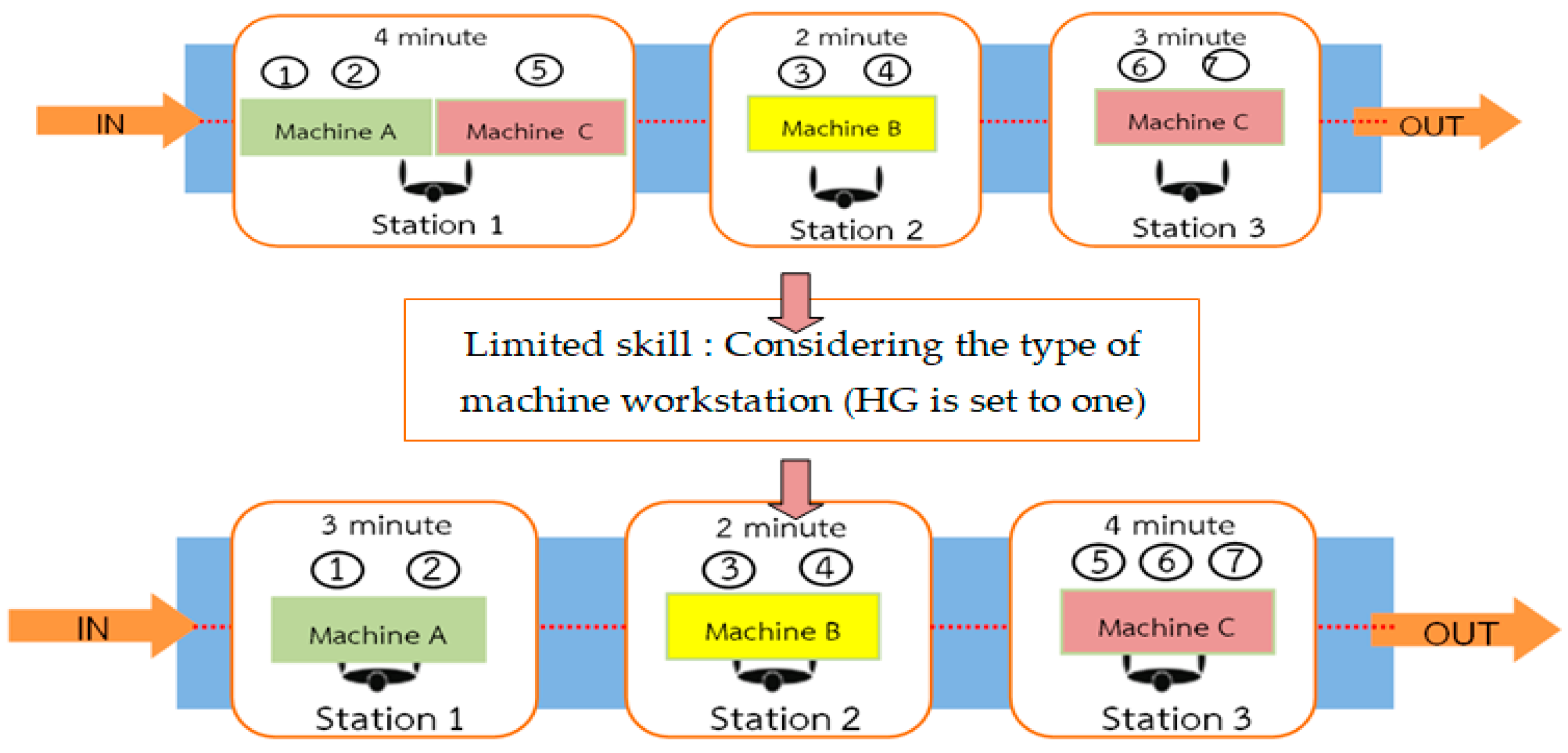
The simple assembly line balancing problem type 2 (SALBP-2) is an extension of (SALBP) that aims to minimize the cycle time (c) for a given number of workstations. In fact, the garment industry or various industries have to use machines for production, but the work procedures are different and so the machines used are different. The workers may not be able to work on many different machines due to the workers’ capability. Therefore, the work procedures and the number of machines that are assigned to the workstation need to be consistent because this may affect the production system, production cycle and the efficiency of the assembly line.

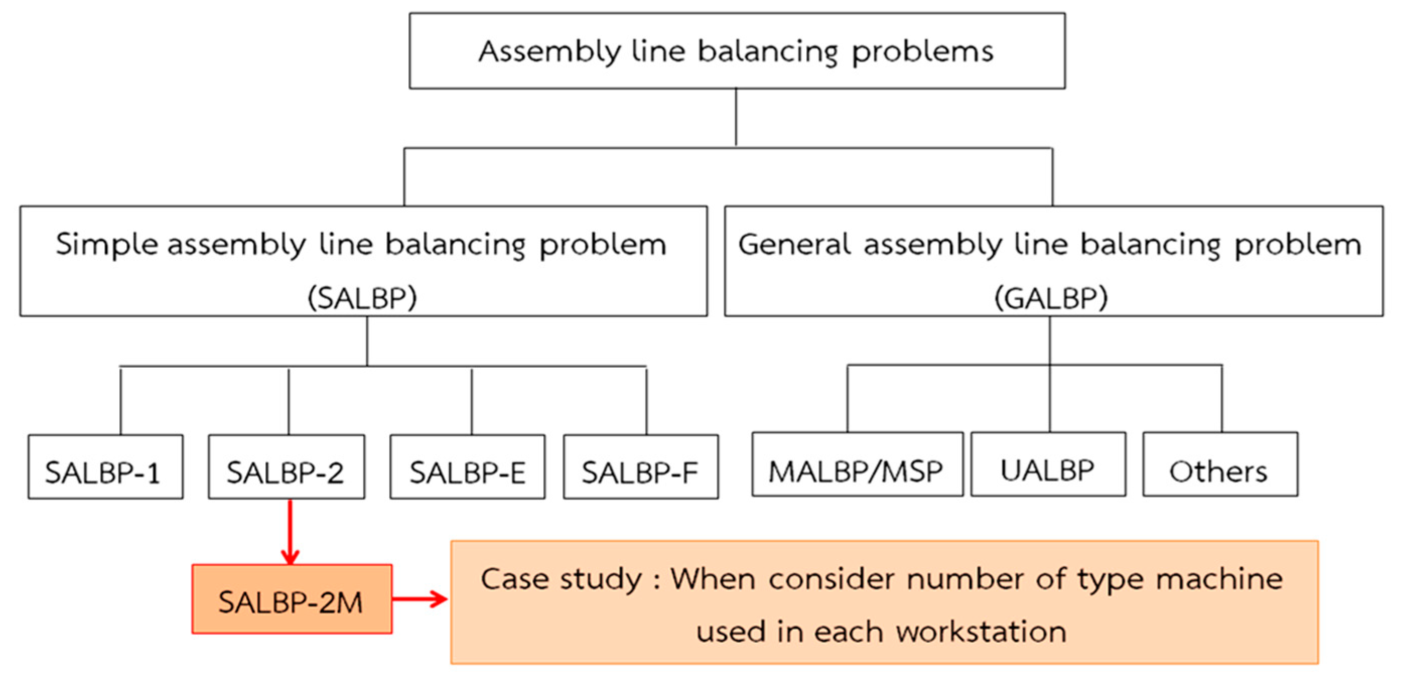
Thus, this research aims to solve a special case of the simple assembly line balancing type 2 problem (SALBP-2). The proposed problem aims to minimize the cycle time considering the number and types of machines for each workstation (SALBP-2M), as shown in Figure 1. Akpýnar (2017) [3] has formerly studied the simple assembly line balancing type 2 problem (SALBP-2). The paper presents type 2 datasets of the benchmark, the objective of which was a minimized cycle time. A large neighbor search method was applied as the solution approach. Then, the computation performance was compared with the type 2 datasets of the benchmark. In this paper, a mathematical model is formulated with the objective function of cycle time minimization. The model was tested by LINGO, which is an exact software method. A special constraint is considered by the number of machines assigned to each workstation, which needs to be consistent. This turns the problem into one suitable for real world operation. Moreover, we apply a new method, called the Variable Neighborhood Strategy Adaptive Search (VaNSAS), which is based on the metaheuristic to solve SALBP-2M. This is a new metaheuristic that aims to find solutions in a wider and more suitable area to obtain the best solution. Previously, the case study had no methods for solving problems but only used experience to solve problems appropriately. The main contributions of this paper are twofold. Firstly, the formulated problem is from a real case study in the Ubon Ratchathani province of Thailand. The objective is to minimize the cycle time and consider the number and types of machines for each workstation. Secondly, this paper presents a new metaheuristic, VaNSAS, which does not appear in any paper published in the literature for SALBP.

The method presented in this research consists of six sections, namely the introduction, literature review, mathematical model formulation and problem definition, computational framework and results, conclusions, and finally, future research.

2. Literature Review

In the early 1900s, Henry Ford studied and presented assembly line balancing. After that, in 1954, 1955, and 1956, assembly line balancing was extensively studied [4,5,6]. In 1995, Salveson was the first person to name assembly line balance as the assembly line balance problem (ALBP). Since then, many researchers have studied, developed, and presented various methods to solve assembly line balancing problems in different forms [7].

The assembly line balancing problem, when solved, could help to increase process flow and allow the average production time of each workstation to be equal, and not lead to idle periods and thus increase the cycle time. Assembly line balancing problems can be classified by the type of problem [8,9], as shown in Figure 1 [10,11].

The simple assembly line balancing problem is an assembly line in the production of a single product, as shown in Figure 1. This problem can be divided into four types, which are SALBP-1, to minimize workstations (m), SALBP-2, to minimize cycle time (c), SALBP-E, for finding the optimum efficiency of the assembly line, and SALBP-F, to make the assembly line of procedures in each workstation balanced.

The general assembly line balancing problem (GALBP) is considered a problem that is not included in the simple assembly line balancing problem (SALBP) [12]. This problem can be divided into 3 types, namely, MALBP, which concerns assembly lines with the production of a mixed product and multiple models, the U-line assembly line balancing problem (UALBP), where the worker can work on both sides of a U-shaped assembly line, where this problem is also divided into three types, such as UALBP-1 to minimize workstations (m), UALBP-2 to minimize cycle time (c), and UALBP-E for finding the optimum efficiency of the assembly line. Finally, the third type is an assembly line balancing problem with a wide scope, which may be considered according to other conditions.

It has been said by Gutjahrand and Nemhauser [13] that the assembly line balancing problem can be considered to be NP-hard, and is also complicated when considering multiple objectives at the same time, taking a long time to find the optimal answer. Thus, some researchers have become interested in studying and developing methods to find answers in this regard [10,14,15]. The present research studies the minimization of cycle time in a simple assembly line balancing problem type 2, with limited types of machines, carried out via a VaNSAS method. The simple assembly line balancing problem type 2 has not been widely studied compared with the field of assembly line balancing problem type 1. Thus, researchers have been interested in studying and solving these problems.

In the simple assembly line balancing problem type 1, researchers have been interested in studying and solving problems by presented heuristic methods. Grzechca (2014) [16] presented Ranked Positional Weight (RPW) to reduce the number of workstations. The results showed that the RPW could solve the problem well. Pape (2014) [17] presented the heuristics and lower bounds for the problem. The results showed that the heuristics and lower bounds method could solve the problem well and was the most effective in this regard. The work carried out by Kamarudin et al. (2018) [18] presented a mathematical model with resource constraints. The study found that the mathematical model could minimize the resources and decrease costs. In addition, the metaheuristics methods presented by Ayazi et al. (2011) [19] presented the genetic algorithm (GA) for multi-objective decision-making. The study found that the genetic algorithm could solve the problem well. Parawech et al. (2014) [20] presented differential evolution (DE) in a case study on a garment factory. The study found that DE couldreduce workstations and increase the efficiency of the assembly line. The work carried out by Pitakaso (2015) [21] presented a DE method, finding that the method could resolve the problem. Pitakaso and Sethanan (2015) [22] presents a modified-DE for assembly line balancing with a limit on the number of machine types. The study found that the modified-DE was able to solve the assembly line with a limit of the machine types, as well as minimize workstations. The work carried out by Antoine et al. (2016) [23] presented an iterative local search (ILS) for a dynamic assembly line rebalancing problem. The study found that the method could solve the problem well.

In the simple assembly line balancing problem type 2, researchers have been interested in studying and solving problems by presenting heuristic methods. Kilincci (2010) [24] presented a Petri net-based heuristic method for a simple assembly line balancing problem type 2, in which the objective was to minimize the variations in workloads among the workstations, finding that the method could solve the problem well. The work carried out by Umarani and Valase (2017) [25] presented lean manufacturing techniques for simple assembly line balancing problem type 2, finding that it could reduce the production time and that the productivity per hour was increased. The work carried out by Zhang et al. (2018) [26] presented a heuristic algorithm by mathematical model for a two-sided assembly line with multiple objectives. The study found that the designed heuristic algorithm could resolve the problem well. In addition, the metaheuristics methods presented by Sikora et al. (2015) [27] presented a genetic algorithm (GA), finding that the algorithm was effective in resolving the problem and could find good answers. Lei and Guo (2016) [28] displayed a VNS method for the second type of the two-sided assembly line. The study found that the method was effective for finding the optimal answer. The work presented by Akpýnar (2017) [3] applies an LNS method. The study found that the method was effective in seeking a good solution. The work carried out by Li et al. (2019) [29] employed simulated annealing (SA) for an assembly line balancing problem with multiple operators. The study found that the method could minimize the cycle time and assign a different number of workers to workstations.

From the review of related studies, it has been found that the metaheuristics methods were effective for solving this problem. Many researchers have been interested in studying the solution of these problems by using many methods, such as GA, DE, VNS and LNS. Moreover, there are studies and solutions that are similar to this paper, considering the number and types of machines for each workstation, although these were for SALBP-1 using the DE method to solve the problem. For the SALBP-2, there is no research that considers the number and types of machines for each workstation. Therefore, this article has applied the DE method into a new VaNSAS method to solve the SALPB-2problem, considering the number and machine type for each of workstations (SALBP-2M). The VaNSAS method is shown in Section 4.

3. Problem Definitions and Mathematical Model

This section presents the construction of the problem definitions and the mathematical model formulation, which is applied to compute the simple assembly line balancing problem type 2 in a garment industry case study, which is defined as shown in Section 3.1 and Section 3.2.

3.1. Problem Definitions

This research attempts to solve the problem of a case study of the garment industry in Ubon Ratchathani in Thailand. The research problem is the extended version of the simple assembly line balancing problem type 2 (SALBP-2). We consider a restricted number and type of machines for working operations due to the limitation of worker skill. The precedence diagram of the short-sleeved clothes of the case study which comprises 36 workflow steps is shown in the Appendix A.

The assembly line balancing problem type 2 of the garment industry aims to minimize the cycle time (c) by assigning the tasks to a given number of workstations (here, a set of 23 stations with cycle time of 2 minutes is used).

Table 1. Result of the task assignments of the proposed problem in the case study.

Workstations	Task	Task Time (Minute)	Machine Type	Workstations	Task	Task Time (Minute)	Machine Type
1	1	1.05	Hand work	13	21	0.22	SNA(2)
2	18, 12, 9	1.90	4OL	14	3	0.22	SNA(1)
3	13	0.65	FLA(1)	15	29, 16, 4	1.30	4OL
4	19	0.78	FLA(2)	16	17	0.38	FLA(2)
5	14	0.63	4OL	17	22, 11, 23	1.74	4OL
6	15	0.60	FLA(2)	18	24	0.67	SNA(2)
7	10	0.25	SNA(2)	19	32, 26	1.49	4OL
8	7, 2, 5, 6	1.41	SNA(1)	20	34	0.43	SNA(2)
9	27	0.68	SNA(2)	21	33, 35	1.13	SNA(1)
10	28, 20	0.72	4OL	22	30, 31	0.74	SNA(2)
11	25	0.42	SNA(2)	23	36	1.23	DNN
12	8	0.40	SNA(1)

shows the results of the assignment, where the workstations, number of tasks, and maximum number of machines in each workstation (HG) are set to one.

To consider the number and types of machines for each workstation, the HG is set to one. This has been done as a single worker has limited skill and cannot use more than a predefined maximum number of machines in those workstations, as shown in Figure 2.

3.2. Mathematical Model

Indices

• $n$ index of tasks n when n = 1, 2, …, N
  $m$ index of task m when m = 1, 2, …, M
• $s$ index of workstations s when s = 1, 2, …, S
• $g$ index of machines g when g = 1, 2, …, G

Parameters

• $N$ Total number of tasks and N equals to M
• $S$ Total number of workstations
• $\mathrm{HG}$ Highest number of machines in each station.
• $P{T}_n$ Processing time of task n
• $P_{nm}=\{\begin{array}{ll}1& if task n is predecessor of task m\\ 0& otherwise\end{array}$.
• $W_{ng}=\{\begin{array}{ll}1& if task n uses machine g to produce\\ 0& otherwise\end{array}$.

Decision Variables

• $C$ Cycle time
• $X_{ns}=\{\begin{array}{ll}1& if task n is assigned to workstation s\\ 0& otherwise\end{array}$
• $Y_{sg}=\{\begin{array}{ll}1& if \mathit{machine} g is \mathit{operated} on workstation s\\ 0& otherwise\end{array}$
• $O_s=\{\begin{array}{ll}1& if workstation s is opened\\ 0& otherwise\end{array}$

Objective function

$$\mathrm{Min}Z=C$$

(1)

Subject to

$${\displaystyle \sum }_{s=1}^S{X}_{ns}=1\forall n=1,2,\dots ,N$$

(2)

$${\displaystyle \sum }_{s=1}^S\left[\left({sX}_{ms}\right)-\left({sX}_{ns}\right)\right]\ge 0\forall n=1,2,\dots ,N;m=1,2,\dots {,M\mathrm{and}P}_{nm}=1$$

(3)

$${\displaystyle \sum }_{n=1}^N\mathrm{P}{T}_n{X}_{\mathrm{ns}}\le \mathrm{C}\forall s=1,2,\dots ,S$$

(4)

$$O_s\le O_{s-1}\forall s=2,\dots ,S$$

(5)

$${\displaystyle \sum }_{n=1}^N{\mathrm{W}}_{gn}{X}_{\mathrm{ns}}\le {\mathrm{Y}}_{sg}\forall s=1,2,\dots ,S;\forall g=1,2,\dots ,G$$

(6)

$${\displaystyle \sum }_{g=1}^G{\mathrm{Y}}_{sg}\le O_{\mathrm{s}}HG\forall s=1,2,\dots ,S$$

(7)

$$X_{ns}\in \left\{0,1\right\}\forall n,s$$

(8)

$${\mathrm{Y}}_{\mathrm{sg}}\in \left\{0,1\right\}\forall s,g$$

(9)

$${\mathrm{O}}_{\mathrm{s}}\in \left\{0,1\right\}\forall s$$

(10)

The mathematical model shown above for the simple assembly line balancing problem type 2, when considering the number and type of machines used in each workstation, is present by Equation (1), which presents an objective function to minimize cycle time (c). Equation (2) is the process that controls the task that must be assigned to only one workstation. Equation (3) presents the condition for each task step when assigned to the workstation, without contradiction with the precedence relationship between tasks. Equation (4) controls the processing time of each task on a particular workstation, which must not exceed the cycle time. Equation (5) is the opening of a new workstation, which shall not open before the next workstation if the previous workstation was not functioning before. Equation (6) is the equation to determine the assignment conditions of the task to the workstation when using the machinery of that task assigned to such a workstation. Equation (7) is the equation specifying the conditions to arrange the machinery to the workstation, whereby each machine can be assigned to the workstation, which must not exceed the total number of machines allowed. Equations (8)–(10) are binary variables.

4. Proposed Method

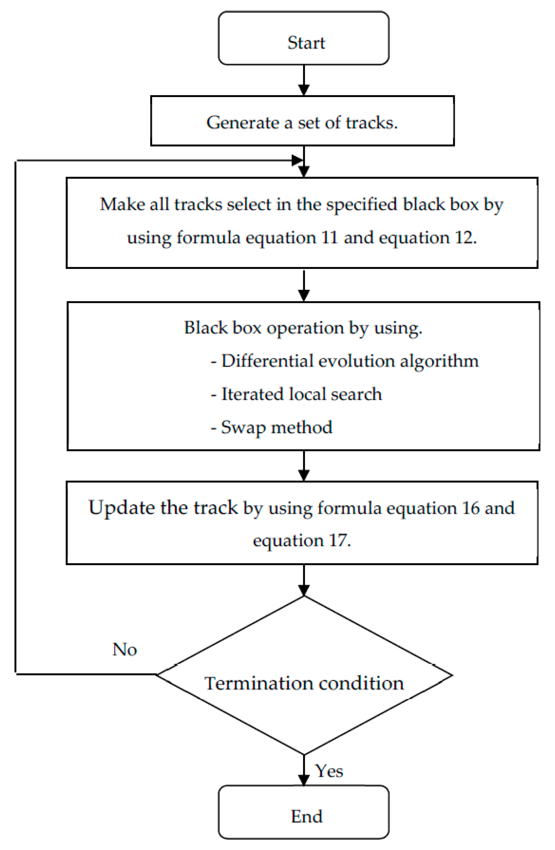
VaNSAS is a new metaheuristic method which aims to allow the algorithm to search in many different areas in order to obtain the most optimal solution, which can gain more diversification or intensification all the time, depending on the black box procedures. In general, the algorithm of VaNSAS consists of five steps, as shown as Figure 3.

Figure 3 shows the procedure of VaNSAS that comprises five steps, which are (1) generating a set of tracks; (2) all tracks select the specified black box; (3) operating in the designed three black boxes; (4) updating the track; and (5) repeating steps 2 to 4 until the termination condition is met. Due to VaNSAS operating with the real number, the track transforming process will be used to transform the real number into the solution for the problem. All steps of VaNSAS can be explained as follows.

The method of VaNSAS has been developed and applied to find the optimal solution for the simple assembly line balancing problem type 2, concerning the garment industry case study. The operation method of VaNSAS is to find the answer by generating a set of tracks and apply the black box method to find the optimal solution of each track update. Then, the method compares the tracks to select the best one.

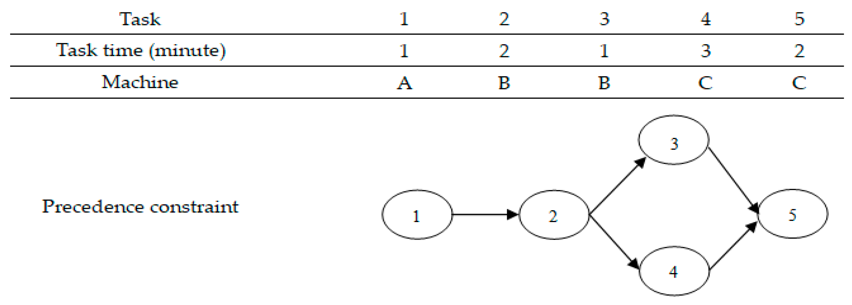
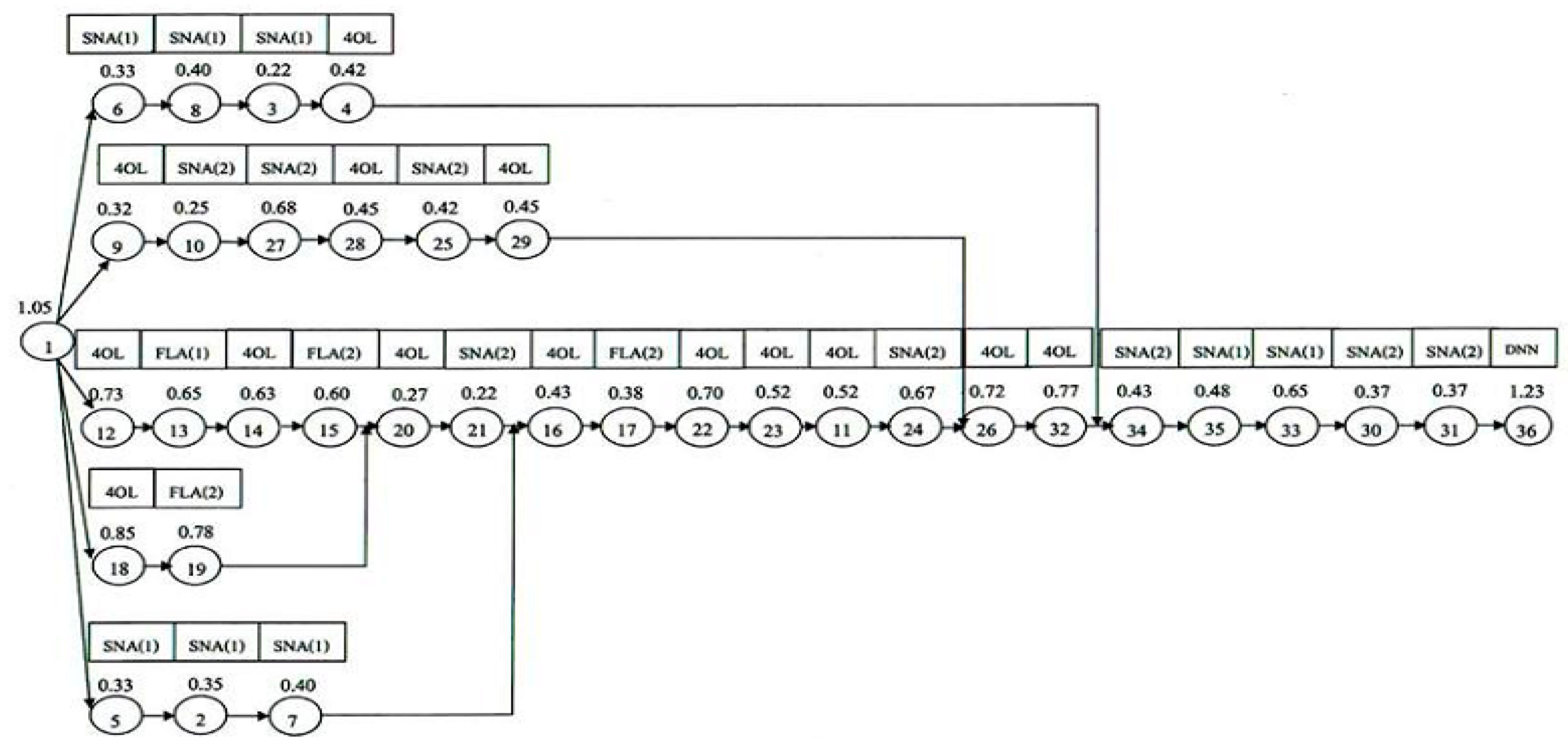
Figure 4 shows the sequence of work steps before and after using circular symbols for connections between parts of work processes and arrow symbols for determining the operating direction. In Figure 3, the numbers inside the circles represent the sequence of work steps with the production cycle not exceeding 5 min.

4.1. Generate A Set of Tracks

This task is used to represent a set of tracks for the solution in terms of a random number. For example, in Figure 3, the precedence diagram shows the previous sequence of simple assembly line balancing. There are six tasks and three types of machinery to be assigned to a track. A track can consist of 5 elements. Each element represents a specific task. The examples of random tasks are shown in

Table 2. The track and the element value.

	Element Value	1	2	3	4	5
Track	1	0.26	0.51	0.11	0.08	0.40
	2	0.03	0.38	0.09	0.54	0.33
	3	0.65	0.30	0.23	0.11	0.59
	4	0.12	0.83	0.42	0.14	0.33
	5	0.34	0.15	0.38	0.70	0.63

.

Table 2 shows the initial answer generation process. After receiving the initial answer set of the random numbers 0 to 1, the next answer set is chosen and entered into the process of transforming the track.

Track Transforming Process (TTP)

The track transforming process of the random numbers, as shown in Table 1, is carried out in order to solve the problem of simple assembly line balancing. The relevant information needs to be informed of 3 explanations, as shown in

Table 3. Touring process of the simple assembly line balancing.

Random	0.26	0.51	0.11	0.08	0.40
Task	1	2	3	4	5
Task time	1	2	1	3	2
Machine	A	B	B	C	C

.

(1) Rank the workflow by sorting the track element’s value. For example, for the first element’s value, the first step uses the first track value, which is 0.26. Then, the second step uses the second track value, which is 0.51, and the third step uses the third track value, which is 0.11, etc.

(2) Assign work steps to the workstation. These steps must not contradict the conditions of the sequence of work relationships before and after, as well as not exceeding the production cycle time.

(3) Define the machine type of each step for the workstation, whereby only 1workstation can have 1 type of machine.

4.2. Make All Tracks Select in The Specified Black Box

Operating in the black box means choosing the answer search method designed for finding the answer to each problem in order to obtain the optimal answer. In this research, we have designed the algorithm to be used in 3 black boxes, i.e., a differential evolution algorithm (DEA), iterated local search (ILS) method, and a swap method (Swap). The track selects a black box, individually performing the black box searching process by using the following formula:

$$P_{bt}=\frac{F{N}_{bt-1}+\left(1-F\right)A_{bt-1}+K{I}_{bt-1}}{{{\displaystyle \sum }}_{bt=1}^n{W}_{bt}}$$

(11)

$$P_{bt}=\frac{F{N}_{bt-1}+\left(1-F\right)A_{bt-1}+K{I}_{bt-1}+MR}{{{\displaystyle \sum }}_{bt=1}^n{W}_{bt}}$$

(12)

where P_bt is the probability for selection black box b in iteration t; N_bt−1 is the number of tracks that have selected black box b in the previous t iteration; A_bt−1 is the average objective value of all tracks that selected black box b in the previous iteration; I_bt−1 is a reward value, where it is incremented by 1 if a black box finds the best solution in the last iteration, but it is set to zero if this is not the case. Additionally, W_bt is the weight of black box b, F is the scaling factor (F = 0.1197), K is the parameter factor (K = 0.5564), M is the parameter factor (M = 0.1), and R is the random number which has a value of 0 to 1.

4.3. Black Box Operation

In this research, we have designed the algorithm to use aforementioned three black boxes. As the first calculation is not required for use in the formula when selecting the operating black box, this work uses a method of calculating the selection of black box b from random numbers (0–1) in order to select the operation of each black box b by specifying the probability of selecting the black box to be equal to 0.33, then calculating to find the cumulative probability of each black box b as follows:

(a)

Differential evolution algorithm (DEA): There is a cumulative probability range between 0.01–0.33.

(b)

Iterated local search (ILS): There is a cumulative probability range between 0.34–0.67.

(c)

Swap method: There is a cumulative probability range between 0.68–1.00.

Then, a number between 0–1 is randomly selected for each track, as shown in

Table 4. Operate the black box.

Track						Random	Black Box
1	0.26	0.51	0.11	0.08	0.40	0.05	DEA
2	0.03	0.38	0.09	0.54	0.33	0.93	Swap
3	0.65	0.30	0.23	0.11	0.59	0.49	ILS
4	0.12	0.83	0.42	0.14	0.33	0.38	ILS
5	0.34	0.15	0.38	0.70	0.63	0.27	DEA

, in order to select the operation of the black box

Table 4 shows the results of the black box selection when entering the black box workflow. Tracks 1 and 5 select the black box DEA method, due to the random number which is in the range between 0.01–0.33. Track 2 selects swap method, which has a random number range between 0.68–1.00. Tracks 3 and 4 select the ILS method, which has a random number range between 0.34–0.67. When the selection of the black box for all tracks has finished, we move on to the next step.

The black box workflow is the process of applying all 3methods for finding the answer, which is how the black box works, which is explained as follows.

4.3.1. Differential Evolution Algorithm (DEA)

This is a method that has a similar evolution to the genetic algorithm (GA), but the DEA has a non-complex structure that can use real numbers for calculation, which is different from Gas in terms of getting the right value without the need to convert decision variables into binary numbers. Differential evolution is more effective in finding answers than other methods, such as those first used by Storn and Price (1997) [30] for solving the complex problem. Therefore, this method is suitable for development and application. There are 5 steps of differential evolution (DE), which are shown as follows:

Step 1: Initial population.

This step consists of creating the initial population of the differential evolution algorithm to be used the initialization of step 1, which generates a set of tracks from Table 4 by selecting track 1, as shown in

Table 5. Initialization carried out in order to generate a set of a tracks for simple assembly line balancing.

Target Vector (Xi,G + 1)	0.26	0.51	0.11	0.08	0.40
Task	1	2	3	4	5
Task time	1	2	1	3	2
Machine	A	B	B	C	C

.

In Table 5, the random number data of the target vector are sorted from small to large. Then, we choose the work step from the smallest value that is put into the workstation first, which must not go against the condition of the relationships of the precedence diagram, as well as not exceeding the cycle time (cycle time = 5), as shown in Table 5.

Table 6. Task assignment at a workstation (cycle time = 5).

Workstation	1		2		3
Target vector (Xi,G + 1)	0.26	0.51	0.08	0.11	0.40
Task	1	2	4	3	5
Task time	1	2	3	1	2
Machine	A	B	C	B	C
Cycle Time	3		4		2

shows the task assignment of a workstation with a cycle time of 5 minutes, in which there are 5 workstations.

Step 2: Mutation.

The purpose of the mutation process is to change the values into coordinates referred to as a weighting factor (F), to create a result of anew answer that is different from the initial answer of the initial vector. In this regard, Gamperleet al. (2002) [31] has said that a value of 0.6 for F is a good initial choice of starting value for finding appropriate answers. This is used to calculate the mutant vector from Equation (13), as shown in

Table 7. Mutation (V_{i,G + 1}) (F = 0.6).

Task	1	2	3	4	5
Target vector (Xi,G + 1)	0.26	0.51	0.11	0.08	0.40
Mutant vector (Vi,G + 1)	0.32	0.49	0.33	0.20	0.17

.

$$V_{i, G+1}=X_{r_1^i, G}+F\left(X_{r_2^i, G}-X_{r_3^i, G}\right)$$

(13)

Table 7 shows the calculation of the mutant vector from three randomly selected target vectors from Table 4 by substituting the values into Equation (10). For example, task 1 is 0.51 + (0.6× (0.08 − 0.40)) = 0.32, whereby the selected target vector must not be the same as the target vector that has already been selected. Then, this result is entered into the coordinate recombination process.

Step 3: Recombination.

The recombination process can increase the diversity of answers, and this step provides the trial vector. The method of recombination used was binomial crossover, as shown in Equation (14), producing answers as shown in

Table 8. Recombination (U_i,G) (CR = 0.3).

Task	1	2	3	4	5
Target vector random	0.17	0.28	0.64	0.02	0.71
Target vector (Xi,G + 1 )	0.26	0.51	0.11	0.08	0.40
Mutant vector (Vi,G + 1 )	0.32	0.49	0.33	0.20	0.17
Trial vector (Ui,G)	0.32	0.49	0.11	0.20	0.40

. Then, the new answers have been brought to be organized into the workstation, as displayed in

Table 9. Task assignment at a workstation (cycle time = 5).

Workstation	1		2		3
Target vector (Xi,G + 1)	0.32	0.49	0.11	0.20	0.40
Task	1	2	3	4	5
Task time	1	2	1	3	2
Machine	A	B	B	C	C
Cycle Time	3		4		2

. A crossover rate value of 0.3 should be chosen, which is a good initial starting value for finding optimal solutions Gamperleet al. (2002) [31]. Here, we calculate the recombination vector (U_i,G) via Equation (11), as shown in Table 8.

$$U_{i, G}=\{\begin{array}{l}{V}_{i,G}^j, if \left(rand\left(j\right)\le CR\right)\\ X_{i,G}^j,if \left(rand\left(j\right)\ge CR\right)\end{array}$$

(14)

Table 8 presents the results of recombination by binomial crossover, which considers and compares the coordinate exchanges as in Equation (14). If the target vector random value is less than or equal to the CR value, the value of the mutant vector is selected; however, if the target vector random is greater than CR, the target vector value is selected. For example, task 1 has a target vector random of 0.17, which is less than the CR of 0.3, so choose the value of the mutant vector equal to 0.32. If task 3 has a target vector random of 0.64, which is greater than the value of 0.3, the value of target vector is chosen, etc. Then, the trial vector that goes into the workstation, as assigned by the task procedures for workstations, considering the smallest trial vector value, which is assigned to workstations first. The details of this are shown in Table 9.

Table 9 shows the task assignment of the workstations with a cycle time of 5 minutes, where there are 3 workstations. The next process is the selection.

Step 4: Selection.

The selection process is chosen only for the optimal answer by comparing the trial vector with the target vector. In the case where the value of the trial vector is larger than the target vector, it shall be replaced by the trial vector, as in Equation (15), which shall obtain the next version in order to find the best answer.

$$X_{i, G+1}=\{\begin{array}{ll}{U}_{i, G+1},& if {\displaystyle \int }\left(U_{i, G+1}\right)\le {\displaystyle }\left(X_{i, G}\right)\\ X_{i, G},& \mathrm{Otherwise}\end{array}$$

(15)

Step 5: Here, steps two to four are repeated, which shall be iteratively executed until the predefined number of iterations has been executed. The next black box procedure used in our method is the iterated local search (ILS) method.

4.3.2. Iterated Local Search (ILS)

ILS is a metaheuristic method developed from basic local search (BLS), which was first provided by Lourenço et al. [32]. Namely, the method searches for the specific answer that disturbs the old answer to obtain a new area to find the answer, then repeats continuously until reaching the designated stop condition. The general concept of ILS is composed of 6 steps, detailed as follows:

• Step 1: Generate the initial solution. This step is selected from the track conversion process, as shown in Table 3, and selects the initial answer from the random selection of black boxes, which is track 3, to operate in the ILS method.
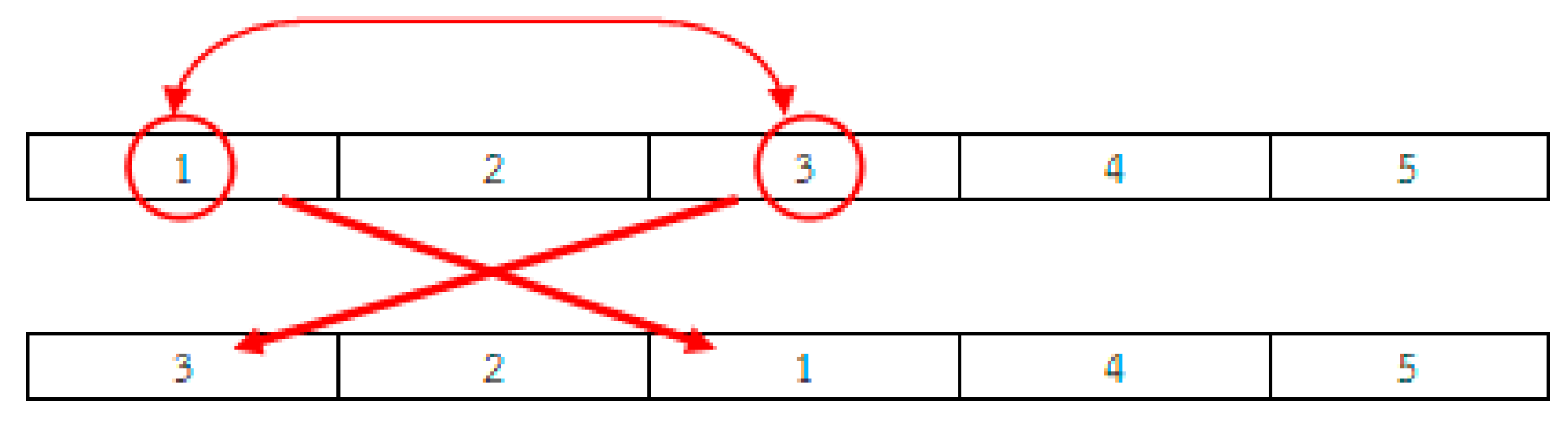
• Step 2: Swap between steps until all positions are exchanged (Figure 5).
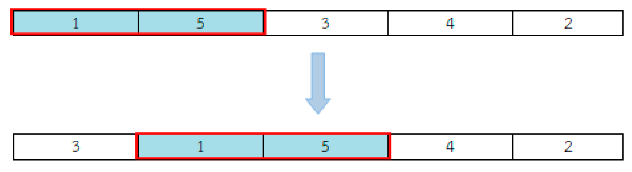
• Step 3: Perturbation by randomly selecting the 2 consecutive positions. Then, choose the random insertion position.
• Step 4: Insert 2 positions in step 3 into the track, then obtain a new solution (Figure 6).
• Step 5: To employ the new solution to organize work steps into the workstation, which must not contradict the conditions of the sequence of the tasks and machine types.
• Step 6: Repeat steps 2 through to 5 until the stopping criteria are reached.

4.3.3. Swap Method (Swap)

The swap method is a well-known local search method that is capable of improving an answer to gain a better answer. Specific answer improvements can be made in many ways, depending on the type of problem to be solved. The popular methods of improvement for specific topical solutions are Swap, 2-Opt, and customer-exchange, etc. The swap method is a popular method that researchers have studied and applied to solve problems, for instance, in Srisuwandee and Pitakaso (2012) [33], the method is applied to find solutions to the vehicle routing problem when using ant colony optimization, concerning a Jiaranai Drinking Water Company case study, using alternate methods to improve the quality of answers. Besides, Chantarasmai and Sindhuchao (2012) [34] has employed the improvement of vehicle routing with the iterated local search method in a case study of Tongnamkeang shop, taking the position swap method to enhance the quality of the answer, etc. The swap method is composed of 5 steps, detailed as follows:

• Step 1: Generate the initial solution. This step is selected from the track conversion process shown in Table 3, which is track 2whenoperating with the Swap method.
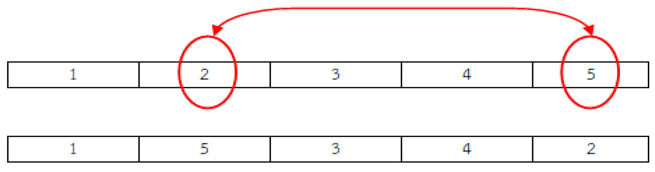
• Step 2: Randomly select a track position, where swapping is carried out by randomly choosing position 1 or track 1, then randomly choosing a position, which is randomly picking position 3 or track 3, to swap with track 1.
• Step 3: Randomly swap position, then obtain a new solution (Figure 7).
• Step 4: Give the new task solutions to organize the steps for the workstations, which must not contradict the conditions of the sequence of tasks, the before–after working relationship, and the type of machinery in each workstation.
• Step 5: Redo steps 2 to 4 until the stopping criteria are reached.

An example of swapping is shown in Figure 6.

4.4. Update The Track

Update the track and all information using the formula as in Equations (16) and (17).

$$Z_{ijt+1}=Z_{ijt}+\alpha \left(Z_{ijt}^{pb}-Z_{ijt}\right)+\left(1-\alpha \right)\left(Z_{ijt}^{gb}-Z_{ijt}\right)$$

(16)

$$Z_{ijt+1}=Z_{ijt}+\alpha \left(Z_{2jt}-Z_{ijt}\right)+\left(1-\alpha \right)\left(Z_{3jt}-Z_{ijt}\right)$$

(17)

where $Z_{ijt+1}$ denotes the value of track i, element j, and iteration t + 1, respectively. Additionally, $\alpha$ is the predefined parameter ($\alpha$ equal to 0.1), $Z_{ijt}$ is the randomly selected track, $Z_{ijt}^{pb}$ is the personal best track, and $Z_{ijt}^{gb}$ is the global best solution.

4.5. Repeat Steps 2 to 4.

Repeat steps 2 to 4 until the termination condition is met. The stopping criteria here is the maximum number of iterations, which is set to 500 iterations (resulting from the preliminary test).

5. Computational Framework and Result

The proposed algorithm has been coded and simulated in Visual Studio C# using a PC with an Intel Core™ i3-4010U 1.70 GHz CPU and 5 GB of RAM, which has been compared with the solutions obtained from the LINGO version 11 software. The best objective was compared in case the optimal solution was not obtained within a limited time. The algorithms were tested for five runs, then the best solution among the five runs was reported. Each method was set to have 500 iterations as the stopping criterion. The VaNSAS method has been tested with 5.1 datasets of SALBP-2 and SALBP-2M, for three groups of the test instances, i.e., (1) small-sized instances containing 8 tasks, (2) medium-sized instances containing 29 tasks, and (3) large-sized instances contain 111 tasks, including the case study problems. The computational framework is shown in

Table 10. Details of the test instances.

Instance	Workstations	Task	Instance	Workstations	Task
Small (S1)	3	8	Medium (M5)	11	29
Small (S2)	4	8	Medium (M6)	12	29
Small (S3)	5	8	Medium (M7)	13	29
Small (S4)	6	8	Large (L1)	13	111
Small (S5)	7	8	Large (L2)	14	111
Small (S6)	8	8	Large (L3)	15	111
Small (S7)	9	8	Large (L4)	16	111
Medium (M1)	7	29	Large (L5)	17	111
Medium (M2)	8	29	Large (L6)	18	111
Medium (M3)	9	29	Large (L7)	19	111
Medium (M4)	10	29	Case study	23	36

.

The proposed algorithms consisted of two methods of black box selection and updating the track. The combinations of the proposed algorithms were named VaNSAS.1 to VaNSAS.4. Details of these algorithms as shown in

Table 11. Definition of the proposed algorithms.

Algorithms	Definition of the Proposed Algorithm
VaNSAS.1	Using operate the black box, Equation (11) + update the track, Equation (16)
VaNSAS.2	Using operate the black box, Equation (11) + update the track, Equation (17)
VaNSAS.3	Using operate the black box, Equation (12) + update the track, Equation (16)
VaNSAS.4	Using operate the black box, Equation (12) + update the track, Equation (17)

.

Datasets of SALBP-2 and SALBP-2M

Datasets for SALBP-2 and SALBP-2M have been tested and the results are shown in

Table 12. Computational results of the instance of SALBP-2.

Instance	Workstations	Task	Cycle Time (Minute)
			SALBP-2	LINGO	VaNSAS.1	VaNSAS.2	VaNSAS.3	VaNSAS.4
S1	2	8	1.77	1.77 Opt	1.77	1.77	1.77	1.77
S2	3	8	1.28	1.28 Opt	1.28	1.28	1.28	1.28
S3	4	8	1.05	1.05 Opt	1.05	1.05	1.05	1.05
S4	5	8	1.05	1.05 Opt	1.05	1.05	1.05	1.05
S5	6	8	1.05	1.05 Opt	1.05	1.05	1.05	1.05
S6	7	8	1.05	1.05 Opt	1.05	1.05	1.05	1.05
S7	8	8	1.05	1.05 Opt	1.05	1.05	1.05	1.05
M1	7	29	0.68	0.68 Opt	0.68	0.68	0.68	0.68
M2	8	29	0.62	0.62 Opt	0.62	0.62	0.62	0.62
M3	9	29	0.57	0.57 Opt	0.57	0.57	0.57	0.57
M4	10	29	0.53	0.53 Opt	0.53	0.53	0.53	0.53
M5	11	29	0.47	0.47 Opt	0.47	0.47	0.47	0.47
M6	12	29	0.45	0.45 Opt	0.45	0.45	0.45	0.45
M7	13	29	0.42	0.42 Opt	0.42	0.42	0.42	0.42
L1	13	111	192.83	192.93 Obj	192.83	192.87	192.83	192.92
L2	14	111	179.82	179.32 Obj	179.13	179.21	179.15	179.20
L3	15	111	167.98	167.83 Obj	167.32	167.35	167.35	167.35
L4	16	111	157.27	157.06 Obj	156.90	156.90	156.90	156.97
L5	17	111	147.67	147.90 Obj	147.73	148.18	147.73	148.20
L6	18	111	139.62	141.40 Obj	139.62	139.65	139.65	139.67
L7	19	111	133.17	132.35 Obj	132.47	132.73	132.73	132.73

Note: ^Opt is the optimal solution found by LINGO and ^Obj is the best objective found within 7200 minutes.

,

Table 13. Statistical test results of the results shown in Table 12.

	VaNSAS.1	VaNSAS.2	VaNSAS.3	VaNSAS.4
LINGO	0.142	0.326	0.199	0.361
VaNSAS.1	-	0.093	0.206	0.060
VaNSAS.2	-	-	0.236	0.101
VaNSAS.3	-	-	-	0.155

,

Table 14. Computational results of the instance of SALBP-2M.

Instance	Workstations	Task	Randomly Machine		Cycle Time (Minute)
				SALBP-2	LINGO	VaNSAS.1	VaNSAS.2	VaNSAS.3	VaNSAS.4
S1	2	8	3	1.77	1.77 Opt	1.77	1.77	1.77	1.77
S2	3	8	2	1.28	1.28 Opt	1.28	1.28	1.28	1.28
S3	4	8	1	1.05	1.05 Opt	1.05	1.05	1.05	1.05
S4	5	8	2	1.05	1.05 Opt	1.05	1.05	1.05	1.05
S5	6	8	3	1.05	1.05 Opt	1.05	1.05	1.05	1.05
S6	7	8	3	1.05	1.05 Opt	1.05	1.05	1.05	1.05
S7	8	8	2	1.05	1.05 Opt	1.05	1.05	1.05	1.05
M1	7	29	2	0.68	0.68 Opt	0.68	0.68	0.68	0.68
M2	8	29	3	0.62	0.62 Opt	0.62	0.62	0.62	0.62
M3	9	29	1	0.57	0.57 Opt	0.57	0.57	0.57	0.57
M4	10	29	1	0.53	0.53 Opt	0.53	0.53	0.53	0.53
M5	11	29	2	0.47	0.47 Opt	0.47	0.47	0.47	0.47
M6	12	29	1	0.45	0.45 Opt	0.45	0.45	0.45	0.45
M7	13	29	3	0.42	0.42 Opt	0.42	0.42	0.42	0.42
L1	13	111	3	192.83	234.70 Obj	228.03	228.22	228.18	228.22
L2	14	111	2	179.13	216.48 Obj	208.23	208.35	208.50	208.50
L3	15	111	1	167.32	200.30 Obj	194.85	194.62	194.67	194.85
L4	16	111	3	156.90	166.85 Obj	164.78	164.82	164.78	164.86
L5	17	111	1	147.73	163.07 Obj	157.18	157.32	157.32	157.32
L6	18	111	2	139.62	155.70 Obj	146.72	147.00	147.23	147.18
L7	19	111	1	132.47	150.03 Obj	145.77	145.86	145.86	145.97
Case study	23	36	1	2.00	1.23 Opt	1.23	1.23	1.23	1.23

Note: ^Opt is the optimal solution found by LINGO and ^Obj is the best objective found within 7200 minutes.

,

Table 15. Statistical test results of the results shown in Table 14.

	VaNSAS.1	VaNSAS.2	VaNSAS.3	VaNSAS.4
LINGO	0.009	0.009	0.009	0.009
VaNSAS.1	-	0.176	0.131	0.027
VaNSAS.2	-	-	0.227	0.038
VaNSAS.3	-	-	-	0.127

,

Table 16. Different ratios (%diff) the instances of SALBP-2M.

Instance	Workstations	Task	Randomly Machine	%diff
				LINGO	VaNSAS.1	VaNSAS.2	VaNSAS.3	VaNSAS.4
S1	2	8	3	0.00	0.00	0.00	0.00	0.00
S2	3	8	2	0.00	0.00	0.00	0.00	0.00
S3	4	8	1	0.00	0.00	0.00	0.00	0.00
S4	5	8	2	0.00	0.00	0.00	0.00	0.00
S5	6	8	3	0.00	0.00	0.00	0.00	0.00
S6	7	8	3	0.00	0.00	0.00	0.00	0.00
S7	8	8	2	0.00	0.00	0.00	0.00	0.00
M1	7	29	2	0.00	0.00	0.00	0.00	0.00
M2	8	29	3	0.00	0.00	0.00	0.00	0.00
M3	9	29	1	0.00	0.00	0.00	0.00	0.00
M4	10	29	1	0.00	0.00	0.00	0.00	0.00
M5	11	29	2	0.00	0.00	0.00	0.00	0.00
M6	12	29	1	0.00	0.00	0.00	0.00	0.00
M7	13	29	3	0.00	0.00	0.00	0.00	0.00
L1	13	111	3	21.71	18.25	18.35	18.33	18.35
L2	14	111	2	20.85	16.25	16.31	16.40	16.40
L3	15	111	1	19.71	16.45	16.32	16.35	16.45
L4	16	111	3	6.34	5.02	5.05	5.02	5.07
L5	17	111	1	10.38	6.40	6.49	6.49	6.49
L6	18	111	2	11.52	5.09	5.29	5.45	5.41
L7	19	111	1	13.26	10.04	10.11	10.11	10.19
Case study	23	36	1	−38.50	−38.50	−38.50	−38.50	−38.50
Average				2.97	1.77	1.79	1.80	1.81

,

Table 17. Statistical test results of the results shown in Table 16.

	VaNSAS.1	VaNSAS.2	VaNSAS.3	VaNSAS.4
LINGO	0.010	0.010	0.009	0.010
VaNSAS.1	-	0.164	0.137	0.033
VaNSAS.2	-	-	0.230	0.037
VaNSAS.3	-	-	-	0.137

,

Table 18. Computational time results of instances of SALBP-2M.

Instance	Workstations	Task	Randomly Machine	Computational Time (Minute)
				LINGO	VaNSAS.1	VaNSAS.2	VaNSAS.3	VaNSAS.4
S1	2	8	3	0.0003	0.001	0.001	0.001	0.001
S2	3	8	2	0.0003	0.002	0.003	0.002	0.002
S3	4	8	1	0.0003	0.0037	0.0038	0.0033	0.0040
S4	5	8	2	0.0003	0.0067	0.0070	0.0058	0.0038
S5	6	8	3	0.0003	0.0070	0.0088	0.0058	0.0030
S6	7	8	3	0.0003	0.0053	0.0078	0.0125	0.0072
S7	8	8	2	0.0003	0.0062	0.0063	0.0058	0.0047
M1	7	29	2	0.0012	0.0002	0.0015	0.0008	0.0008
M2	8	29	3	1.0013	0.0010	0.0015	0.0005	0.0007
M3	9	29	1	0.5500	0.0008	0.0008	0.0005	0.0005
M4	10	29	1	9.1667	0.0007	0.0010	0.0007	0.0002
M5	11	29	2	1.2833	0.0008	0.0012	0.0005	0.0002
M6	12	29	1	26.90	0.0010	0.0008	0.0005	0.0002
M7	13	29	3	0.0002	0.0007	0.0007	0.0005	0.0003
L1	13	111	3	7200	2.3833	3.6200	2.7167	2.2583
L2	14	111	2	7200	5.4928	6.9667	5.2217	5.4373
L3	15	111	1	7200	2.6220	3.0918	2.8353	2.9405
L4	16	111	3	7200	6.5668	6.1255	8.0582	5.0395
L5	17	111	1	7200	1.8217	2.9365	2.5732	1.5185
L6	18	111	2	7200	2.6708	3.5578	2.6708	2.2237
L7	19	111	1	7200	4.2725	5.7000	4.2725	4.5575
Case study	23	36	1	1979.72	1.16	1.37	1.18	1.21
Average				2382.66	1.23	1.52	1.34	1.15

and

Table 19. Statistical test results of the results shown in Table 18.

	VaNSAS.1	VaNSAS.2	VaNSAS.3	VaNSAS.4
LINGO	0.003	0.003	0.003	0.003
VaNSAS.1	-	0.022	0.147	0.291
VaNSAS.2	-	-	0.248	0.008
VaNSAS.3	-	-	-	0.191

.

From Table 12, it can be seen that LINGO could find the optimal solution in the small-and medium-sized instances, but for the large-sized instance, LINGO could find only the best objective, respectively. On the other hand, all proposed methods could find the optimal solution.

The results were analyzed using statistical methods for performance comparison, shown in Table 13. The results show that all proposed methods were non-significantly different when compared to the solution from LINGO. Moreover, all proposed methods were also insignificantly different when compared to each other.

The results given in Table 13 show that LINGO and VaNSAS.1 to VaNSAS.4 were non-significantly different from each other.

As shown in Table 14, LINGO could find the optimal solution in the small- and medium-sized instances included in the case study. However, for the large-sized instance, LINGO could only find the best objective, respectively. On the other hand, we can see that, when considering the number of machines to be added into the constraint of the task assignment in each workstation, the cycle time increased forSALBP-2.The results were analyzed using the statistical methods shown in Table 15 and a different ratio (%diff) of the cycle time of SALBP-2M (Equation (18)) was found, as shown in Table 16.

The results were analyzed using statistical methods for performance comparison in Table 15. The results show that LINGO and VaNSAS.1 to VaNSAS.4 were significantly different from each other.

Table 16 presents the %diff of the cycle time of SALBP-2M by each algorithm when compared to the result from the original SALBP-2. Here, %diff was calculated using Equation (18):

$$\%diff= \frac{(C{t}^{new}-C{t}^{oid})}{C{t}^{oid}}\times 100\%$$

(18)

where $C{t}^{new}$ is the cycle time of the proposed algorithm generated by solving SALBP-2M and $C{t}^{old}$ is the cycle time of the proposed method of SALBP-2.

From Table 16, SALBP-2M had the limitation of the maximum number of machines, where the cycle time would increase from the SALBP-2 version. This meant that it was harder to solve than that of SALBP-2.

Figure 8 shows the percentage differences (%diff) of the instances of SALBP-2M. The computational results show VaNSAS.1has the lowest percentage difference when compared with other methods: the percentage difference is 1.77. The VaNSAS.2–VaNSAS.4 methods have average differences of 1.79, 1.80 and 1.81, respectively. All proposed VaNSAS results are less than the result from LINGO, which is 2.97.

Finally, the statistical test was tested with the result given in Table 16. If each method performed differently while solving a given instance, which was the modified version of SALBP-2 when using a paired t-test, the result was recorded. This is shown in Table 17.

The results were analyzed using statistical methods for performance comparison in Table 17, with different %diff values in different instances of SALBP-2M. The results show that all proposed methods were significantly different from each other when compared to the solution found by LINGO. Moreover, all of the proposed methods were also insignificantly different. This means that the proposed methods are high-performance metaheuristic methods, capable of finding the near-optimal solution.

From the computational results shown in Table 18 and Figure 9, all of the proposed methods can be seen to find a better solution than that of the best solution obtained by LINGO version 11, which required an average of 2382.66 min, while the proposed methods used only 1.23 min, 1.52 min, 1.34 min, and 1.15 min, respectively, to find such a good solution.

According to Table 19, the results of the response processing time found that the method presented to VaNSAS.1 to VaNSAS.4 gave different results from the best solution provided by LINGO, which means that the proposed method is effective and able to find a good answer to the proposed problems.

The case study here included the 36 tasks and the aim was to minimize the cycle time of the system. The problems assigned these tasks into 22 workstations with 2-minute cycle times. The precedent diagram for the case study is shown in the Appendix A. The type of machine in each workstation did not exceed one.

The computational results of the case study when using VaNSAS (example result from VaNSAS.1) are shown in

Table 20. Task assignment for workstations after adjustment.

Workstation	Task	Time (Minute)	Idle Time (Minute)	Machine
1	1	1.05	0.18	Hand work
2	6, 8, 3	0.95	0.28	SNA(1)
3	4, 12	1.15	0.08	4OL
4	13	0.65	0.58	FLA(1)
5	14	0.63	0.60	4OL
6	15	0.60	0.63	FLA(2)
7	18	0.85	0.38	4OL
8	19	0.78	0.45	FLA(2)
9	5, 2, 7	1.08	0.15	SNA(1)
10	9, 20	0.59	0.64	4OL
11	10, 21, 27	1.15	0.08	SNA(2)
12	28, 16	0.88	0.35	4OL
13	17	0.38	0.85	FLA(2)
14	22, 23	1.22	0.01	4OL
15	11	0.52	0.71	4OL
16	24, 25	1.09	0.14	SNA(2)
17	29, 26	1.17	0.06	4OL
18	32	0.77	0.46	4OL
19	34	0.43	0.80	SNA(2)
20	35, 33	1.13	0.10	SNA(1)
21	30, 31	0.74	0.49	SNA(2)
22	36	1.23	0.00	DNN
	Total	19.04	8.02

.

Table 20 shows the cycle time, which reduced to 1.23 minutes. The results of the simple assembly line balancing problem type 2 of the case study, before and after adjustment, are shown in

Table 21. Computational results of the case study.

No.	Consideration	LINGO	VaNSAS.1	VaNSAS.2	VaNSAS.3	VaNSAS.4
1	Workstations	22	22	22	22	22
2	Cycle time (minute)	1.23	1.23	1.23	1.23	1.23
3	Assembly line efficiency (percent)	70.36	70.36	70.36	70.36	70.36
4	Computational time (minute)	1979.72	1.16	1.37	1.18	1.21

, as obtained by the VaNSAS method. The results of testing all of the proposed methods are shown, along with those found by LINGO version 11 when solving the problems in the case study. We ran LINGO version 11 for 1979.72 minutes and the best objective was found during the simulation run, which is reported in Table 21.

Table 21 presents the results of the VaNSAS method when applied to the simple assembly line balancing problem type 2 of the case study. The results show that the VaNSAS method can reduce the cycle time from 2.00 minutes to 1.23 minutes. The effectiveness of the assembly line increased here from 41.49% to 70.36%. The VaNSAS method was able to solve the assembly line balancing problem type 2 and could find the optimal solution as well. Therefore, the VaNSAS method is efficient for application in solving the assembly line balance problem and has a much lower computational time.

6. Conclusions and Future Research

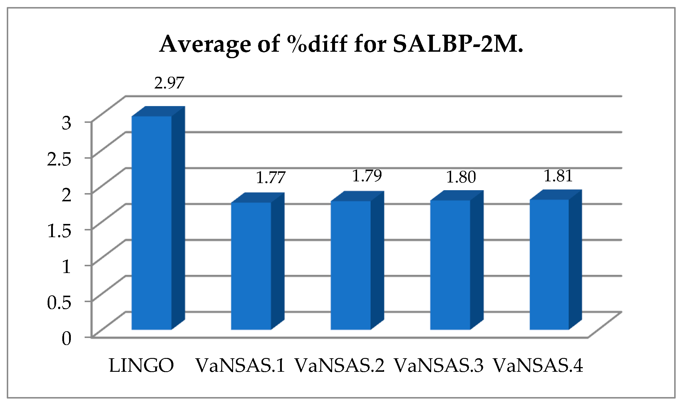
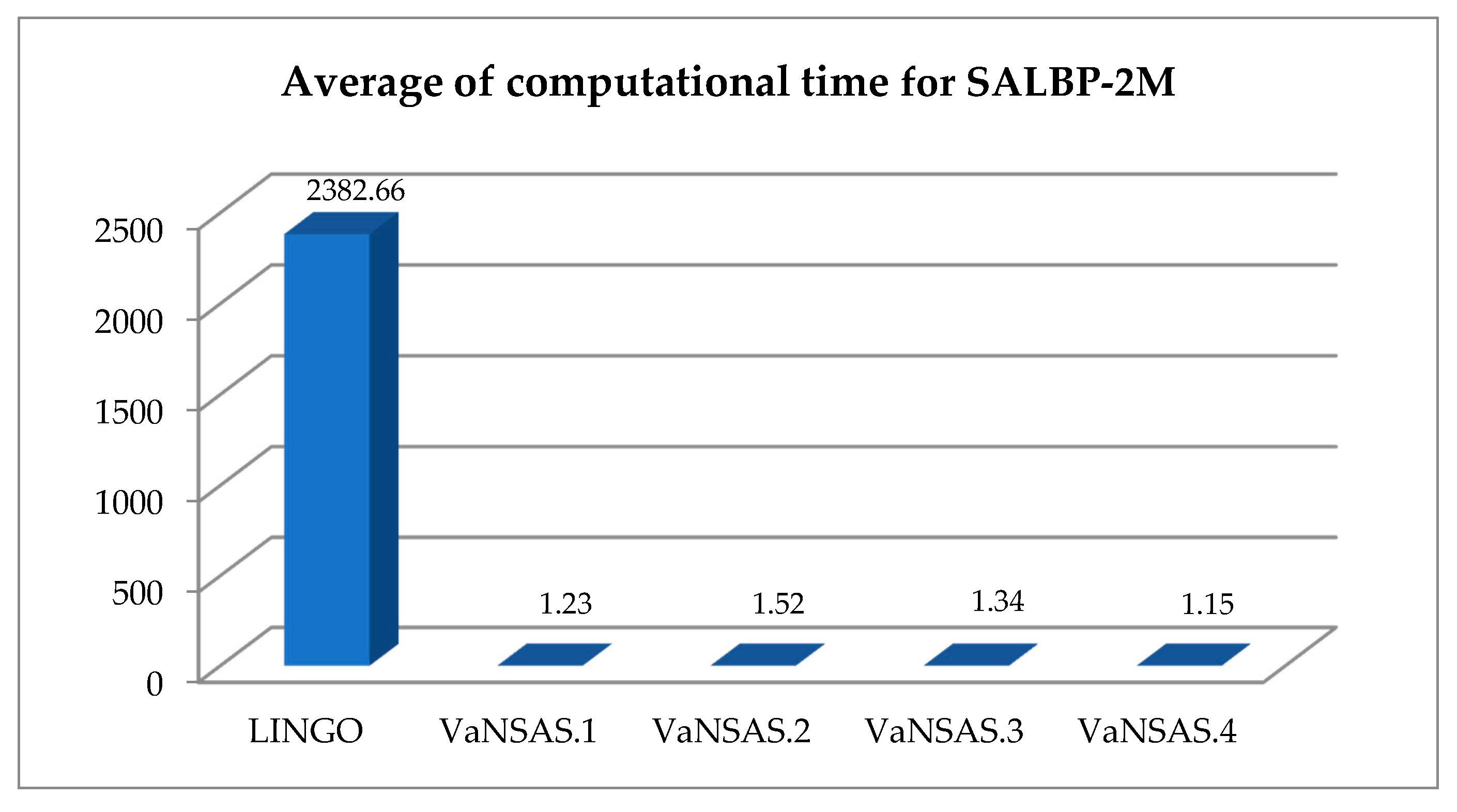
This research has focused on solving the minimization of cycle time for a simple assembly line balancing problem type 2, considering a garment industry case study (SALBP-2M). We have presented a variable neighborhood strategy adaptive search algorithm (VaNSAS), composed of five steps, i.e., generating a set of tracks, making all tracks operate in the specified black box, operating the black box via the three black-box methods, which have been modified from the original version of them, and, therefore, effective neighborhood strategies have been created for use as improvement tools of VaNSAS. The neighborhood strategies used in this article include a differential evolution algorithm (DEA), iterated local search (ILS) method, and a swap method (Swap). The fourth step consists of updating the track and repeating steps two to four until the termination condition is met. We have divided the proposed VaNSAS method into four algorithms, i.e., VaNSAS.1, VaNSAS.2, VaNSAS.3, and VaNSAS.4, respectively, in order to evaluate the performance of the various black box selections and update the tracks.

The computational results show that VaNSAS.1outperformed the other proposed algorithms of black box selection (Equation (11)) and the other track update formulas (Equation (16)) due to VaNSAS.1 providing a better answer and taking less time to process the answer than the other methods. The VaNSAS concept was derived from the combination of all three methods in the black box, with random problems choosing the black box method to solve the problem. Moreover, it depended on the idea that the track be made more intense, because it was the weight calculation of the best objective obtained by choosing the black box for the given operation. A further objective was to improve the track by choosing only the track from the best objective, and the good objectives received for improvement were used in the next round. Therefore, the black box method generated the best answer and the best track updates were more likely to be repeatedly chosen, which is effective in regard to resolving problems.

The VaNSAS method outperformed the best-known heuristic methods (LINGO version 11), finding the optimal solution of SALBP-2 and SALBP-2M datasets. The case study results show that the proposed VaNSAS method has reduced the cycle time to 1.23 minutes and increased the assembly line effectiveness to 70.36%, indicating that the proposed VaNSAS method could be applied to effectively solve the assembly line balance problem.

The researchers recommend considering other additional factors in future research, for instance, the study of employee skills and performance, and the study of the capability of each type of machine used in the production process, applying the principles of open innovation. This may be in the form of software or applications to collect data, or the exchange of information between organizations using production planning, or solutions to various problems that occur.

References

1. Chesbrough, H.; Crowther, A.K. Beyond high tech: Early adopters of open innovation in other industries. RD Manag. 2006, 36, 229–236. [Google Scholar] [CrossRef]
2. Kumar, N.; Mahto, D. Assembly Line Balancing: A Review of Developments and Trends in Approach to Industrial Application. Glob. J. Res. Eng. Ind. Eng. 2013, 13, 29–50. [Google Scholar]
3. Akpýnar, Þ. Large neighbourhood search algorithm for type-II assembly line balancing problem. PamukkaleUnivMuhBilimDerg. 2017, 23, 444–450. [Google Scholar] [CrossRef] [Green Version]
4. Bryton, B. Balancing of A Continuous Production Line. Master’s Thesis, Northwestern University, Evanston, IL, USA, June 1954. [Google Scholar]
5. Salveson, M.E. The assembly line balancing problem. J. Ind. Eng. 1955, 6, 18–25. [Google Scholar]
6. Jackson, J.R. A Computing Procedure for a Line Balancing Problem. Manag. Sci. 1956, 2, 261–271. [Google Scholar] [CrossRef]
7. Erel, E.; Sarin, S.C. A survey of the assembly line balancing procedures. Prod. Plan. Control. 1998, 9, 414–434. [Google Scholar] [CrossRef] [Green Version]
8. Scholl, A.; Becker, C. State-of-the-art exact and heuristic solution procedures for simple assembly line balancing. Eur. J. Oper. Res. 2006, 168, 666–693. [Google Scholar] [CrossRef]
9. Becker, C.; Scholl, A. A survey on problems and methods in generalized assembly line balancing. Eur. J. Oper. Res. 2006, 168, 694–715. [Google Scholar] [CrossRef]
10. Kriengkorakot, N.; Pianthong, N. The Assembly Line Balancing Problem: Review articles*. KKU Eng. J. 2007, 34, 133–140. [Google Scholar]
11. Jusop, M.; Ab. Rashid, M.F.F. A review on simple assembly line balancing type-e problem. IOP Conf. Ser. Mater. Sci. Eng. 2015, 100, 012005. [Google Scholar] [CrossRef] [Green Version]
12. Boysen, N.; Fliedner, M.; Scholl, A. A classification of assembly line balancing problems. Eur. J. Oper. Res. 2007, 183, 674–693. [Google Scholar] [CrossRef]
13. Gutjahr, A.L.; Nemhauser, G.L. An Algorithm for the Line Balancing Problem. Manag. Sci. 1964, 11, 308–315. [Google Scholar] [CrossRef]
14. Nearchou, A. Multi-objective balancing of assembly lines by population heuristics. Int. J. Prod. Res. 2008, 46, 2275–2297. [Google Scholar] [CrossRef] [Green Version]
15. Great, O.E.; Offiong, A.N. Productivity improvement in breweries through line balancing Using Heuristic Method. Int. J. Eng. Sci. Technol. 2013, 5, 475–486. [Google Scholar]
16. Grzechca, W. Assembly Line Balancing Problem with Reduced Number of Workstations. IFAC Proc. Vol. 2014, 47, 6180–6185. [Google Scholar] [CrossRef]
17. Pape, T. Heuristics and lower bounds for the simple assembly line balancing problem type 1: Overview, computational tests and improvements. Eur. J. Oper. Res. 2015, 240, 32–42. [Google Scholar] [CrossRef] [Green Version]
18. Kamarudin, N.H.; Ab. Rashid, M.F.F. Modelling of Simple Assembly Line Balancing Problem Type 1 (SALBP-1) with Machine and Worker Constraints. J. Phys. Conf. Ser. 2018, 1049, 012037. [Google Scholar] [CrossRef]
19. Ayazi, S.; Hajizadeh, A.; Nooshabadi, M.; Jalaie, H.; Moradi, Y. Multi-objective assembly line balancing using genetic algorithm. Int. J. Ind. Eng. Comput. 2011, 2, 863–872. [Google Scholar] [CrossRef]
20. Parawech, P.; Pitakaso, R.; Mayachearw, P. Solving an assembly line balancing problem by differential evolution: A case study of a garment factory. Princess Naradhiwas Univ. J. 2014, 6, 92–104. [Google Scholar]
21. Pitakaso, R. Differential evolution algorithm for simple assembly line balancing type 1 (SALBP-1). J. Ind. Prod. Eng. 2015, 32, 104–114. [Google Scholar] [CrossRef]
22. Pitakaso, R.; Sethanan, K. Modified differential evolution algorithm for simple assembly line balancing with a limit on the number of machine types. Eng. Optim. 2015, 48, 1–19. [Google Scholar] [CrossRef]
23. Antoine, M.; El Haouzi, H.; RamdaneCherif, W.; Lounes, B. Iterated Local Search for dynamic assembly line rebalancing problem. IFAC-Pap. OnLine. 2016, 49, 515–519. [Google Scholar] [CrossRef]
24. Kilincci, O. A Petri net-based heuristic for simple assembly line balancing problem of type 2. Int. J. Adv. Manuf. Technol. 2010, 46, 329–338. [Google Scholar] [CrossRef]
25. Umarani, P.; Valase, K. Assembly line balancing in textile industry. Int. J. Sci. Res. Eng. Technol. 2017, 6, 323–330. [Google Scholar]
26. Zhang, Y.; Hu, X.; Wu, C. Heuristic Algorithm for Type II Two-sided Assembly Line Rebalancing Problem with Multi-objective. MATEC Web Conf. 2018, 175, 03063. [Google Scholar] [CrossRef] [Green Version]
27. Sikora, C.G.S.; Lopes, T.C.; Lopes, H.S.; Magatão, L. Genetic algorithm for type-2 assembly line balancing. In Proceedings of the 2015 Latin America Congress on Computational Intelligence (LA-CCI), Curitiba, Brazil, 13–16 October 2015; pp. 1–6. [Google Scholar]
28. Lei, D.; Guo, X. Variable neighborhood search for the second type of two-sided assembly line balancing problem. Comput. Oper. Res. 2016, 72, 183–188. [Google Scholar] [CrossRef]
29. Li, Y.; Wang, H.; Yang, Z. Type II assembly line balancing problem with multi-operators. Neural Comput. Appl. 2019, 31, 347–357. [Google Scholar] [CrossRef]
30. Storn, R.; Price, K. Differential Evolution—A Simple and Efficient Heuristic for global Optimization over Continuous Spaces. J. Glob. Optim. 1997, 11, 341–359. [Google Scholar] [CrossRef]
31. Gamperle, R.; Muller, S.; Koumoutsakos, A. A Parameter Study for Differential Evolution. Adv. Intell. Syst. Fuzzy Syst. Evol. Comput. 2002, 10, 293–298. [Google Scholar]
32. Lourenço, H.R.; Martin, O.C.; Stützle, T. Iterated Local Search. In Handbook of Metaheuristics; Glover, F., Kochenberger, G.A., Eds.; Springer US: Boston, MA, USA, 2003; pp. 320–353. [Google Scholar]
33. Srisuwandee, T.; Pitakaso, R. Solving vehicle routing problem by using ant colony optimization case study in jiaranai drinking water company. KKU Eng. J. 2012, 17, 706–714. [Google Scholar]
34. Chantarasmai, K.; Sindhuchao, S. Improvement of vehicle routes with the iterated local search method case study: Tongnamkeang shop, warinchumrab district, ubonratchathani province. KKU Eng. J. 2012, 17, 850–861. [Google Scholar]
Figure 1. Types of assembly line balancing problems (Kriengkorakot and Pianthong [10]).
Joitmc 06 00021 g001
Figure 2. Example of the simple assembly line balancing problem in the case study.
Joitmc 06 00021 g002
Figure 3. Algorithm of VaNSAS.
Joitmc 06 00021 g003
Figure 4. Diagram of simple assembly line balancing.
Joitmc 06 00021 g004
Figure 5. Swap in ILS.
Joitmc 06 00021 g005
Figure 6. Insertion in ILS.
Joitmc 06 00021 g006
Figure 7. Example of swapping.
Joitmc 06 00021 g007
Figure 8. Percentage different (%diff) the instances of SALBP-2M.
Joitmc 06 00021 g008
Figure 9. The average computational time of the instancesof SALBP-2M.
Joitmc 06 00021 g009