Has Digital Financial Inclusion Narrowed the Urban–Rural Income Gap? A Study of the Spatial Influence Mechanism Based on Data from China

Abstract

Although extant literature has extensively discussed the poverty reduction effect of digital financial inclusion, few papers have explored the association from a spatial perspective. Based on the Peking University Digital Financial Inclusive Index, this study empirically tests the impact of digital financial inclusion on the urban–rural income gap in China. To perform the analysis, this paper employs the spatial Durbin model (SDM) with double fixed effects and a mediating effect model. We find that (1) there is a significant positive spatial correlation between digital financial inclusion and the urban–rural income gap, and both variables have certain spatial agglomeration characteristics; (2) digital financial inclusion has a significant promotion effect and a positive spatial spillover effect on reducing the urban–rural income gap; and (3) the test of the spatial influence mechanism shows that the above effect is achieved by promoting industrial structure upgrading. This paper combines the above results to propose corresponding policy recommendations, which are valuable for other developing countries and emerging economies with similar backgrounds to China.

1. Introduction

Based on the Global Wealth Report 2021 from Credit Suisse, the richest 10% of the world’s population held 82% of the world’s wealth, while the bottom 50% held less than 1% in 2020. This shows that wealth inequality is still widespread worldwide. For China, rapid economic growth has achieved poverty reduction at an unprecedented speed and scale [1], but the income gap persists. According to the National Bureau of Statistics, China’s Gini coefficient, a more broad-based measure of wealth inequality, rose from 0.465 in 2019 to 0.468 in 2020, which is higher than the internationally recognized 0.4 “warning line”. Researchers widely believe that the income gap in China is largely reflected in the urban–rural income gap. For example, Chen et al. [2] argued that the Gini coefficient for urban and rural areas contributes 61.6% to the national coefficient. Wan [3] confirmed that the urban–rural income gap contributes 70–80% of the total and an increasing proportion to the overall regional inequality. Statistics show that China’s urban per capita disposable income was CNY 43,833.8 in 2020, much larger than the rural per capita disposable income of CNY 17,131.5, and the urban–rural income gap increased from CNY 13,190.4 to CNY 26,702.3 in the past decade. Although absolute poverty has been completely eliminated, the problem of the urban–rural income gap is very serious.

There are many factors that lead to the urban–rural income gap, such as urbanization level [4,5], air quality [6], and infrastructure conditions [7]. In this paper, we examine whether digital financial inclusion is also a major factor in determining the urban–rural income gap, which has not been evaluated by prior literature. From the perspective of the financial system, rural residents remain excluded from the traditional banking sector due to high transaction costs, high entry thresholds, and information asymmetry, which can hinder rural economic development and increase income [8]. The concept of “financial inclusion” was formally put forward in 2005 at the conference of the International Year of Microcredit. Its commercial sustainability and equal opportunity principles have made great contributions to many developing countries in solving the problem of financial resource allocation imbalances [9,10]. However, due to the large area and scattered population in China, it is still difficult for financial inclusion institutions to reach target customers, such as remote poor people and small businesses [11]. In recent years, the development of the Internet and digital technology has provided a new way to solve the above difficulties. The 2016 G20 Global Partnership for Inclusive Finance (GPFI) defined the concept of digital financial inclusion as “all actions to promote financial inclusion through the use of digital financial services”, making up for the time cost and geographic spatial limitations of traditional financial institutions in the process of promoting inclusive finance. Digital financial inclusion can meet the needs of 80% of customers who are underserved, according to the Pareto principle, better than traditional finance can. Through the integration of information technology and big data, rural residents can use computers, mobile phones, and other devices to obtain financial services. Digital financial inclusion provides financial funds, such as productive loans, student loans, and agricultural insurance, for the poor to meet their financial needs in production, life, and operation [12,13]. However, it should be recognized that there are certain conditions for the use of digital financial inclusion services, such as the need for residents to have and be able to use digital tools such as smartphones and computers. In fact, there is a huge gap between urban and rural areas in China in terms of digital tools, education level, and digital infrastructure construction. Therefore, whether digital financial inclusion will reduce the urban–rural income gap depends on which group of urban and rural residents benefits more from digital financial inclusion. In addition, from the perspective of space, technological innovation has externalities [14]. The application of digital technology to financial inclusion in the region has a demonstration effect and promotes the development of digital financial inclusion in other related regions [15]. If the spatial correlation between digital financial inclusion and the urban–rural income gap can be confirmed, the spatial characteristics can be used to improve the efficiency of limited financial resources, promote the synergistic development of digital financial inclusion among regions, and give full play to the driving effect of developed regions on the backward and marginal regions through the spatial spillover effect, thus eliminating relative poverty.

Using panel data of 31 provinces (autonomous regions and municipalities) in China from 2011 to 2019, this paper first applies the double fixed effects spatial Durbin model to discuss the effect of digital financial inclusion on the urban–rural income gap, and then employs the mediating effect model to study the transmission mechanism of industrial structure. Digital financial inclusion is measured by the Peking University Digital Financial Inclusion Development Index from the Digital Finance Center of Peking University, and the urban–rural income gap is measured by the ratio of the per capita disposable income of urban residents and rural residents. In addition, three different types of control variables are selected, and three different types of robustness checks and the endogeneity test are performed to ensure that the findings are plausible. The results show that first, there is a significant positive spatial correlation between digital financial inclusion and the urban–rural income gap, and both have certain spatial agglomeration characteristics; Second, digital financial inclusion has a significant promotion effect and a positive spatial spillover effect on reducing the urban–rural income gap; Third, the test of the spatial transmission mechanism shows that digital financial inclusion indirectly narrows the urban–rural income gap by affecting the regional industrial structure.

The significant contributions are as follows. First, this paper discusses the relationship between digital financial inclusion and the urban–rural income gap as well as the transmission mechanism and effects through theoretical analysis and empirical research. These findings provide novel evidence to enrich the relevant literature [16,17]. Second, from the methodology perspective, this paper empirically tests the spatial spillover effect of digital financial inclusion on the urban–rural income gap using the spatial Durbin model. Specifically, the spatial Durbin model combines the spatial error model and the spatial autoregressive model to obtain an unbiased estimate. This paper also adds regional-fixed and time-fixed effects to the model to increase the accuracy of the results. Third, this paper focuses on China, a typical developing country and emerging economy, to serve as an inspiration for countries with similar institutional backgrounds and economic development.

The rest of this paper is organized as follows: the second part is the literature review and theoretical analysis, and three research hypotheses are proposed; the third part introduces the research method, including variables and data, spatial correlation test, and model formulation; the fourth part reports the empirical results and discussion, including the main findings, robustness and endogeneity checks, and the test of spatial influence mechanism; and the fifth part concludes the research, comments on the results, and proposes policy suggestions.

2. Literature Review and Theoretical Analysis

2.1. Digital Financial Inclusion and Urban–Rural Income Gap

There is serious financial exclusion in rural areas of China, which is considered to be one of the important reasons why financial development has not narrowed the urban–rural income gap [18,19,20]. In the process of industrialization and urbanization in China, agricultural production provides significant resources for industrial development. The concentration of social capital in cities restricts the development of rural areas. At the same time, the strict household registration system hinders population mobility between urban and rural areas, which in turn forms an urban–rural dual economic structure, and further gives rise to a dual financial structure [21,22]. Traditional financial institutions allocate limited financial resources to the urban non-agricultural sector, or even close rural networks to reduce operating costs and maximize profits. However, farmers and modern agricultural operators have a strong demand for financing [23]. Rural land resources reallocation, agricultural industrialization operation, and rural environmental management are facing a large credit gap. Therefore, there is an urgent need to explore a new model for rural financial services [24].

The main feature of digital financial inclusion is that it replaces traditional payment with mobile payment, traditional deposit and loan with P2P credit, and traditional securities business with crowdfunding financing, which helps alleviate financial exclusion in rural areas [25,26,27,28,29]. First of all, digital financial inclusion can accurately identify and match scattered and small-scale customers through digital technologies, such as the Internet, artificial intelligence, and big data analysis. It helps to reduce transaction costs in human services, physical networks, etc., thereby promoting rural financial market development and mitigating financial exclusion [30,31]. Secondly, the service coverage and customer groups of digital financial inclusion are more extensive, which provides the possibility for rural residents and families to obtain financial resources. Even in remote rural areas that lack bank networks and ATMs, rural residents can access online financial resources through computers, cell phones, and other communication tools [32,33,34]. The development of Internet technology has reduced the marginal cost of access to financial resources in the long-tail market, greatly alleviating financial exclusion [35]. In addition, digital financial inclusion has changed the financial supply system in the rural financial market, which is mainly dominated by policy-based and commercial finance. This has brought competitive pressure on traditional financial institutions, prompting them to continuously develop new products and services suitable for rural financial needs in order to gain competitive advantages. It has, to a certain extent, promoted the diversification and personalization of rural financial services, and better matched rural financial supply with demand [36,37]. Accordingly, we propose Hypothesis 1.

Hypothesis 1.

Digital financial inclusion can narrow the urban–rural income gap.

2.2. The Spatial Spillover Effect of Digital Financial Inclusion on Urban–Rural Income Gap

From a spatial perspective, as factors of production such as capital, resources, and technology can flow across regions, similar regions exhibit similar characteristics in terms of economic activities [38,39]. Therefore, digital financial inclusion and the urban–rural income gap may be spatially correlated between regions. Firstly, with the improvement of digital technology and the popularization of the Internet, the spatial connection of digital finance in various regions has become closer [40]. Developed regions can easily drive the financial activities of other provinces through spatial spillover [41]. Secondly, the financial intermediation function can effectively promote the upgrading and adjustment of industrial structure in the neighboring regions, which will lead to regional economic restructuring and financial scale development, thus improving resource allocation efficiency and generating spatial spillover effect [42,43]. Furthermore, digital financial inclusion promotes personal consumption and enterprise investment by expanding the coverage of financial services, which in turn drives economic growth [44,45,46]. This growth further generates spatial spillover through production factor flows and trade cooperation, which further boosts economic development in related regions [47,48]. Moreover, although there are still restrictions on the mobility of rural residents under China’s household registration system, the phenomenon of large-scale population mobility between regions is undeniable [49]. On the one hand, the floating population participates in the economic construction of the inflowing regions and contributes directly to the economic growth of the neighboring regions [50]. On the other hand, the floating population achieves financial knowledge spillover through the interactive exchange of cognition and experience with the population in the inflowing regions [51,52]. The above process indirectly improves the financial literacy of rural residents in neighboring areas, enabling them to better participate in financial services, increase their income, and improve the efficiency of financial poverty alleviation.

Without considering the spatial spillover effect mentioned above, the impact of digital financial inclusion on the urban–rural income gap may be underestimated. Therefore, this paper proposes a second hypothesis.

Hypothesis 2.

Digital financial inclusion has a significant positive spatial spillover effect on narrowing the urban–rural income gap.

2.3. Transmission Mechanism: The Mediating Role of Industrial Structure Upgrading

Digital financial inclusion can promote industrial structure upgrading through multiple channels to narrow the urban–rural income gap. First, this paper considers capital formation and production factor input allocation. With the continuous development of the financial system, financial thresholds are reduced [53]. An increasing number of residents, especially in rural areas, have easy access to services from financial institutions [54]. Digital financial inclusion helps financial institutions complete the formation and accumulation of capital, which in turn optimizes the allocation of credit funds among industries [55]. At this point, capital is transferred to the more efficient secondary and tertiary industries, upgrading the industrial structure [56]. The rapid development of nonagricultural industries leads to the gradual replacement of labor-intensive industries by technology- and capital-intensive industries. A large number of surplus rural laborers move to cities, and their salary levels are thus improved [57]. Second, this paper considers the effect of technological innovation. Digital financial inclusion can reform and upgrade traditional industry technology by addressing the financing difficulties of rural small and medium-sized enterprises and emerging enterprises [58,59]. Furthermore, upgrading the industrial structure increases agricultural productivity, thus increasing farmers’ income and narrowing the urban–rural income gap [60,61,62]. Third, this paper considers the consumer demand effect. Currently, emerging finance and traditional finance coexist in the financial market, expanding financial service coverage and diversifying the forms of financial products. Digital financial inclusion can relieve consumers from liquidity constraints through reasonable and efficient resource allocation [63]. Moreover, the expansion of consumer demand promotes the upgrading of the industrial structure and simultaneously narrows the urban–rural income gap [64,65,66].

In addition, financial services, science and technology, labor resources, and other factors involved in digital financial inclusion and industrial structure continue to flow across regions. This brings convenience to related regions in terms of production activities, financial cooperation, and information sharing [67]. This spatial correlation can enable digital financial inclusion to not only provide financial services to local individuals and enterprises but also help neighboring less-developed regions compensate for the lack of financial development and provide financial support for industrial structure transformation and upgrading [68,69]. Accordingly, this paper proposes the following hypothesis:

Hypothesis 3.

Digital financial inclusion affects the urban–rural income gap of the region and related areas through industrial structure upgrading.

3. Methods

3.1. Variables and Data

1. Explained Variable: Urban–Rural Income Gap (URIG). The income gap is mainly reflected in uneven development. Among them, the urban–rural income gap is the most common. Regions with higher economic levels deprive other areas of production factors. As a result, regions or people who do not have a good material foundation can only rely on the assistance of the central or local government. The auxiliary effect of national policies makes their income level only slightly higher than the absolute poverty line, but in fact, they have almost no ability to withstand risks. With reference to Yang et al. [70], we select the ratio of the per capita disposable income of urban residents and rural residents to measure the urban–rural income gap.

2. Core Explanatory Variables: Digital Financial Inclusion (DFI). This paper directly uses the “Peking University Digital Financial Inclusion Development Index” compiled by [71] Guo et al. covering 31 provinces (autonomous regions and municipalities) in mainland China to measure the development level of digital financial inclusion. The index considers three dimensions and a total of 33 specific indicators. It uses the analytic hierarchy process, coefficient of variation method, and other methods for measurement and finally provides a set of data that can basically reflect the current development status and evolution trend of digital financial inclusion in China. We further regress the three secondary subindicators of digital finance coverage (breadth), digital finance use depth (depth), and inclusive digital finance level (level) with the explained variable. Through analysis and comparison, we summarize the influence direction and extent of each indicator to ensure the robustness of the benchmark regression. In the empirical analysis, we perform logarithmic processing on the above data.

3. Other Explanatory Variables (control variables). After comprehensively considering relevant factors that may affect the urban–rural income gap, we draw on the literature [72,73,74,75,76] and mainly set three control variables: economic growth, government behavior, and human capital. The definition of variables is shown in

Table 1. Definition of variables.

Control Variables	Definition
open	ratio of actual amount of foreign investment to GDP
urban	ratio of urban employed population to total population
GDP	log value of per capita GDP
social	ratio of social security and employment expenditures to total fiscal expenditures
fiscal	ratio of local government fiscal revenue to total fiscal expenditures
government	ratio of fiscal expenditures to GDP
edu	ratio of illiterate population to the population aged 15 and over
ageing	ratio of elderly population to working population
unemployment	ratio of unemployed population to working population

. Among the characteristic variables of economic growth, openness (open) to the outside world often promotes local enterprise development and labor employment. This can drive economic growth in the region and reduce poverty levels. With the development of urbanization (urban), the policies related to farmers’ entry into cities have been released, and the labor surplus in rural areas has been gradually alleviated. The gradual advancement of urban modernization has greatly increased the income of residents and the level of social development. The improvement in the regional economic level (GDP) improves the living conditions of residents. In this paper, to eliminate the impact of the difference size of the population in each province, the variable is measured by the log value of the per capita GDP. Among the characteristic variables of government behavior, a higher level of government social assistance (social) means a more sound regional social security and employment policy, which can effectively prevent the occurrence of poverty caused by illness in poor groups. Fiscal freedom (fiscal) mainly measures the financial pressure and self-sufficiency of local governments under the current fiscal decentralization system. Government intervention (government) is expressed by fiscal expenditure divided by regional GDP. At present, whether government intervention has an impeding or boosting effect on narrowing the urban–rural income gap remains to be empirically tested. Among the human capital characteristic variables, educational attainment (edu) may change a person’s health decisions, employment choices, and consumer attitudes, which can have an impact on poverty. Ageing (ageing) from an economic point of view reflects the social consequences of population ageing. Unemployment (unemployment) measures idle labor capacity.

Based on the China Statistical Yearbook published by the National Bureau of Statistics, the empirical analysis uses panel data from 31 provinces (autonomous regions and municipalities) in mainland China from 2011 to 2019. The descriptive statistics of each variable are shown in

Table 2. Variable descriptive statistics.

Variables		Obs	Mean	Std.	Min	Max
Explained Variable	URIG	279	2.6556	0.4217	1.8451	3.9792
Main Explanatory Variables	DFI	279	5.1432	0.6785	2.7862	6.0168
	breadth	279	4.9790	0.8518	0.6729	5.9523
	depth	279	5.1265	0.6487	1.9110	6.0866
	level	279	5.4581	0.7166	2.0255	6.1361
Other Explanatory Variables (control variables)	open	279	0.1117	0.1688	0.0000	1.0084
	urban	279	0.5666	0.1314	0.2271	0.8960
	GDP	279	1.5837	0.4361	0.4969	2.7986
	social	279	0.1270	0.0325	0.0548	0.2747
	fiscal	279	0.4909	0.1997	0.0722	0.9314
	government	279	0.2827	0.2119	0.1103	1.3792
	edu	279	0.0608	0.0620	0.0123	0.4418
	ageing	279	0.1383	0.0341	0.0671	0.2382
	unemployment	279	0.0324	0.0064	0.0120	0.0450

below:

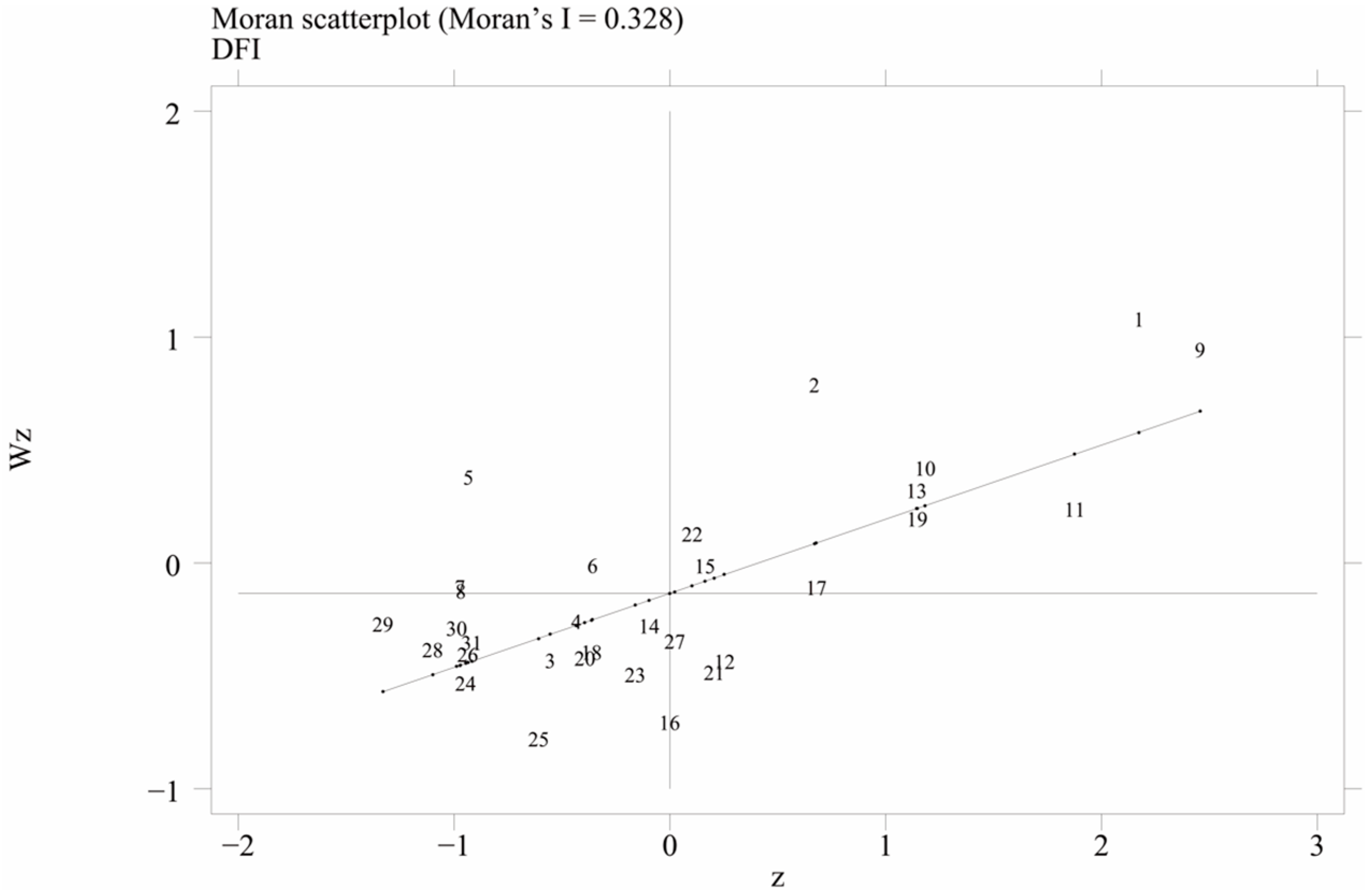
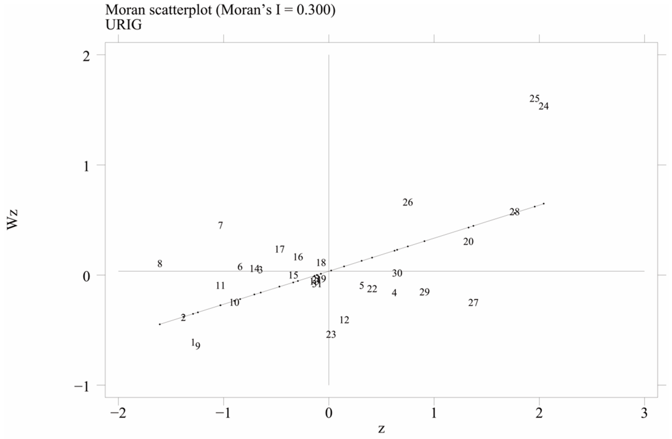
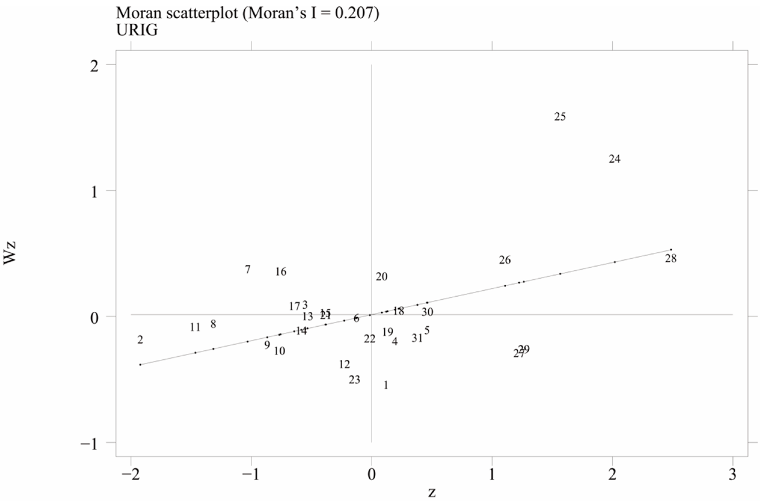
3.2. Spatial Correlation Test

Before establishing the model, we must first test whether there is a spatial correlation between digital financial inclusion and the urban–rural income gap. In spatial econometric analysis, the global Moran’s I and Geary’s C are commonly used to test spatial correlation. The former focuses on describing the global spatial autocorrelation, while the latter is more sensitive to the local spatial autocorrelation. This paper calculates both results of Moran’s I and Geary’s C, which can more comprehensively investigate the spatial correlation of variables. The expressions are shown in Equations (1) and (2):

$$\begin{array}{cc}Moran’s& I\end{array}=\frac{n{\displaystyle \sum _{i=1}^n{\displaystyle \sum _{j=1}^n{w}_{ij}(x_i-\overline{x})}}(x_j-\overline{x})}{{\displaystyle \sum _{i=1}^n{\displaystyle \sum _{j=1}^n{w}_{ij}{\displaystyle \sum _{i=1}^n(x_i-\overline{x})}}}{(x_j-\overline{x})}^2}$$

(1)

$$\begin{array}{cc}Geary’s& C\end{array}=\frac{(n-1){\displaystyle \sum _{i=1}^n{\displaystyle \sum _{j=1}^n{w}_{ij}{(x_i-x_j)}^2}}}{2{{\displaystyle \sum _{i=1}^n{\displaystyle \sum _{j=1}^n{w}_{ij}{\displaystyle \sum _{i=1}^n(x_i-\overline{x})}}}}^2}$$

(2)

Among them, $n$ is the 31 provinces (autonomous regions and municipalities) included in the sample. $w_{ij}$ represents the spatial weight matrix. $x_i$ and $x_j$ represent the digital financial inclusion and the urban–rural income gap of province $i$ and province $j$, respectively. $\overline{x}$ represents the provincial average of the digital financial inclusion and the urban–rural income gap in the same year.

For the setting of the spatial weight matrix, we mainly construct the spatial weight matrix based on the geographical location. The first type is the geographic distance weight matrix ($W_1$), which is often used in spatial measurement. Its element expression is:

$$W_{ij}=\{\begin{array}{ll}\frac{1}{d_{ij}}& i\ne j\\ 0& i=j\end{array}$$

(3)

$d_{ij}$ represents the distance between province $i$ and province $j$, which are calculated from the latitude and longitude coordinates of the corresponding provincial capital city.

The second type is the economic distance weight matrix ($W_2$), and its element expression is:

$$W_{ij}=\{\begin{array}{ll}\frac{1}{\left|E_i-E_j\right|}& i\ne j\\ 0& i=j\end{array}$$

(4)

$E_i$ is the average per capita GDP of province i from 2011 to 2019.

The third type is the nested weight matrix ($W_3$), and its element expression is:

$$W_3=\tau W_1+(1-\tau )W_2$$

(5)

where 0 < $\tau$ < 1 represents the relative importance of the geographical distance weight matrix. Referring to the practice of Shao et al. [77], we assume that τ = 0.5. In the empirical process, we standardize the above weight matrix.

Table 3. Spatial correlation test of the urban–rural income gap and digital financial inclusion under three weights.

Year	URIG						DFI
	Geographic Distance Weight Matrix		Economic Distance Weight Matrix		Nested Weight Matrix		Geographic Distance Weight Matrix		Economic Distance Weight Matrix		Nested Weight Matrix
	Moran’s I	Geary’s C	Moran’s I	Geary’s C	Moran’s I	Geary’s C	Moran’s I	Geary’s C	Moran’s I	Geary’s C	Moran’s I	Geary’s C
2011	0.192 ***	0.775 ***	0.300 ***	0.663 ***	0.246 ***	0.719 ***	0.109 ***	0.838 ***	0.364 ***	0.543 ***	0.237 ***	0.690 ***
2012	0.189 ***	0.782 ***	0.300 ***	0.662 ***	0.245 ***	0.722 ***	0.132 ***	0.835 ***	0.390 ***	0.518 ***	0.261 ***	0.676 ***
2013	0.156 ***	0.820 ***	0.241 ***	0.685 ***	0.199 ***	0.753 ***	0.127 ***	0.841 ***	0.398 ***	0.494 ***	0.263 ***	0.668 ***
2014	0.152 ***	0.826 ***	0.234 ***	0.692 ***	0.193 ***	0.759 ***	0.127 ***	0.847 ***	0.421 ***	0.473 ***	0.274 ***	0.660 ***
2015	0.152 ***	0.821 ***	0.220 ***	0.703 ***	0.186 ***	0.762 ***	0.100 ***	0.881 ***	0.431 ***	0.460 ***	0.266 ***	0.671 ***
2016	0.149 ***	0.824 ***	0.221 ***	0.710 ***	0.180 ***	0.767 ***	0.129 ***	0.854 ***	0.422 ***	0.468 ***	0.275 ***	0.661 ***
2017	0.147 ***	0.829 ***	0.203 ***	0.717 ***	0.175 ***	0.773 ***	0.134 ***	0.845 ***	0.376 ***	0.510 ***	0.255 ***	0.678 ***
2018	0.144 ***	0.830 ***	0.207 ***	0.716 ***	0.176 ***	0.773 ***	0.144 ***	0.837 ***	0.323 ***	0.565 ***	0.234 ***	0.701 ***
2019	0.142 ***	0.832 ***	0.207 ***	0.715 ***	0.175 ***	0.774 ***	0.148 ***	0.832 ***	0.328 ***	0.564 ***	0.238 ***	0.698 ***

Note: *** indicates significance at the level of 1%.

reports the results of the spatial correlation test under the three weights. We can see from the Table that the Moran’s I and Geary’s C of the urban–rural income gap and digital financial inclusion are both less than 1 and pass the significance level test, indicating the existence of a significant positive spatial correlation.

In addition, by comparing the magnitude of Moran’s I, we can see that the urban–rural income gap under the weight of economic distance has the largest spatial correlation with the digital financial inclusion index (Geary’s C yields the same conclusion). The above results illustrate that the spillover caused by economic correlation is more obvious. Therefore, this paper chooses the economic distance weight matrix ($W_2$) to construct the next spatial measurement model.

The global Moran index reflects the overall correlation, and the local spatial correlation of provinces (autonomous regions and municipalities) needs to be further tested. Therefore, this paper continues to use the local Moran’s I scatter plot for analysis (as shown in Figure 1, Figure 2, Figure 3 and Figure 4). China’s digital financial inclusion and the urban–rural income gap are mainly distributed in the first and third quadrants, showing obvious H-H clustering and L-L clustering, with high values closely related to high values and low values closely related to low values. This means that provinces (autonomous regions and municipalities) with high development levels of digital financial inclusion also have relatively high development levels economically; provinces (autonomous regions and municipalities) with low development levels of digital financial inclusion have similarly low development levels in their economically related provinces. In addition, the number of clusters in the third quadrant is significantly higher than that in the first quadrant, indicating that there are still a considerable number of regions where the development level of digital financial inclusion is low. The clustering status of the urban–rural income gap is roughly consistent.

3.3. Model Formulation

Spatial measurement models mainly include the spatial Durbin model (SDM), spatial error model (SEM), and spatial autoregressive model (SAR). Among them, SDM combines the spatial error model and the spatial autoregressive model to obtain an unbiased estimate. Thus, it has a higher degree of explanation. This paper refers to the research of Elhorst [78] to test the applicability of the model, and the results are shown in

Table 4. Applicability test of the spatial econometric model.

Inspection Index	Data	Significant Value
Moran’s I	0.328	0.043
LM test no spatial error	35.486	0.000
Robust LM test no spatial error	47.147	0.000
LM test no spatial lag	33.179	0.000
Robust LM test no spatial lag	44.839	0.000
Hausman test	18.51	0.070
LR test ind both	43.55	0.000
LR test time both	690.16	0.000
LR test spatial lag	86.88	0.000
LR test spatial error	87.89	0.000
Wald test spatial lag	100.58	0.000
Wald test spatial error	95.27	0.000

.

First, the Moran’s I test results indicate that the model has spatial correlation. Second, the LM test results show that both the spatial error model and the spatial autoregressive model are applicable. Third, under the economic distance weight matrix, the Hausman test result of SDM supports the fixed effects spatial measurement model. Fourth, the region and time of SDM and the LR test results regarding double fixed effects all suggest that the double fixed effects of region and time should be controlled in the SDM with fixed effects. Fifth, the Wald test and LR test of SDM under double fixed effects are both significant at the 1% level, so the SDM of double fixed effects cannot be reduced to a spatial error model or a spatial autoregressive model. Hence, this paper uses the SDM with double fixed effects to estimate the poverty reduction effect of digital financial inclusion and its impact mechanism.

The specific econometric model is set as follows:

$$URI{G}_{it}={\omega }_0+\rho W_{2}URI{G}_{it}+{\omega }_{1}DF{I}_{it}+{\omega }_1^{\prime }{W}_{2}DF{I}_{it}+{\omega }_2{X}_{it}+{\omega }_2^{\prime }{W}_2{X}_{it}+{\mu }_i+{\lambda }_t+{\epsilon }_{it}$$

(6)

$URI{G}_{it}$ represents the urban–rural income gap of region i in year t. $DF{I}_{it}$ represents the development level of digital financial inclusion of region i in year t. $X_{it}$ represents additional control variables. ${\mu }_i$ represents the region-fixed effect. ${\lambda }_t$ represents the time-fixed effect. ${\epsilon }_{it}$ is the error term.

4. Results and Discussion

4.1. Main Findings

The SDM estimation results of the two-way fixed effect are shown in

Table 5. SDM estimated results and spatial effects.

Variables	SDM		Effect Decomposition of SDM
	Explanatory Variables	Spatial Variables	Direct Effect	Indirect Effect	Total Effect
DFI	−0.3804 *** (0.0688)	−0.7084 *** (0.1780)	−0.3055 *** (0.0688)	−0.5128 *** (0.1846)	−0.8183 *** (0.1833)
open	−0.2358 (0.1959)	−0.6551 (0.6381)	−0.2528 (0.1938)	−0.6889 (0.7370)	−0.9418 (0.7885)
urban	−2.2467 *** (0.6417)	3.9581 ** (1.8755)	−2.1431 *** (0.6234)	3.9223 ** (1.9611)	1.7792 ** (1.9473)
GDP	−0.1377 ** (0.1000)	−1.6860 *** (0.3881)	−0.1219 ** (0.0974)	−1.7415 *** (0.4308)	−1.8634 *** (0.4521)
social	0.0661 (0.4959)	−4.7409 ** (1.9777)	0.0439 (0.4937)	−5.1054 ** (2.0851)	−5.0614 ** (2.2755)
fiscal	−0.5975 *** (0.2219)	3.1123 *** (0.7107)	−0.5646 *** (0.2186)	3.2991 *** (0.8680)	2.7345 *** (0.9435)
government	−0.6498 (0.3611)	−0.6757 (1.5235)	−0.6200 (0.3718)	−0.7173 (1.7802)	−1.3372 (1.9123)
edu	−0.3511 (0.5528)	−2.7359 (2.4204)	−0.3899 (0.5413)	−3.0954 (2.5582)	−3.4853 (2.7252)
ageing	2.5916 *** (0.5219)	7.0567 *** (2.0157)	2.7031 *** (0.5260)	7.6934 *** (2.2720)	10.3965 *** (2.5744)
unemployment	3.7925 * (2.1177)	3.5081 (7.5710)	3.8899 * (2.1113)	4.4392 (8.2044)	8.3291 (9.1743)
ρ	0.2613 ***
Log-likelihood	331.4688
Fixed Effect	Fixed
Observation	279

Note: *, **, and *** indicate significance at the level of 10%, 5%, and 1%, respectively.

below. Due to the spatial spillover effect, the coefficient of digital financial inclusion can no longer be separately interpreted as a marginal utility for narrowing the urban–rural income gap. Therefore, according to the study of LeSage and Pace [79], the estimation results are decomposed to more accurately explain the direct and indirect effects of digital financial inclusion on poverty reduction.

According to the empirical results, the coefficients of core explanatory variables are negative and significant at the 1% level. The elastic coefficient of digital financial inclusion on the urban–rural income gap is −0.3804, indicating that digital financial inclusion has a significant positive impact on narrowing the urban–rural income gap. Hypothesis 1 is verified. The spatial interaction term coefficient of digital financial inclusion is −0.7084, showing that the development of digital financial inclusion has a significant spatial spillover effect on poverty alleviation in economically relevant provinces. Based on this finding, Hypothesis 2 is verified. Comparing the values of coefficients, it is found that the spatial spillover effect accounts for more than half of the total effect. Ignoring the feature of spatial overflow would underestimate the contribution of digital financial inclusion to poverty alleviation. The Pareto principle of traditional finance means that financial institutions tend to focus the best financial services on the top 20% of customers, while 80% of long-tail customers are excluded. In recent years, due to the continuous development of the Internet and financial system, digital financial inclusion has enabled rural residents, poor people, and other relatively disadvantaged groups to directly obtain financing funds by lowering service thresholds and relaxing credit constraints. Furthermore, digital financial inclusion greatly breaks through the limitations of traditional financial service time and geographic space. Through the technological innovation spillover effect and interregional economic spillover effect, it significantly reduces the urban–rural income gap in related areas.

From the results of control variables, the increase in the level of urbanization (urban) can significantly reduce the urban–rural income gap of the province, but it has the opposite effect on economically-related provinces. Urbanization leads to a large amount of labor force employment, which in turn attracts labor migration from other provinces. The above process contributes to the economic growth of the destination provinces but also increases the urban–rural income gap in the origin provinces. The GDP results are significant, and the indirect effect is greater than the direct effect. At present, trade barriers between various regions in China are gradually being eliminated. The free flow of products and factors not only develops the economy of the province but also drives the economy of the related provinces. The continuous expansion of market demand further promotes employment, thereby reducing poverty. The direct effect of government social assistance is not significant, but the indirect effect is significantly negative, which indicates that social security and employment-related fiscal expenditures need to be strengthened to protect poor groups. The greater the value of fiscal freedom is, the stronger the regional fiscal self-sufficiency. The results show that provinces with high fiscal freedom can reduce the urban–rural income gap. However, the spatial effect result takes the opposite direction. The ageing results are significantly positive. Regardless of whether it is the province or the related provinces, the continuous increase in the proportion of the elderly population has an adverse impact on the progress of the country’s economic level, the improvement in the social security system, and the development of education and culture. The direct effect of the unemployment rate is significantly positive. Employment issues are directly related to the income level of a family. An increase in family income reduces the probability of poverty. In addition, the results of the variables open, government, and education are not significant.

Furthermore, this paper uses the three secondary subindices of the digital financial inclusion index as core explanatory variables for regression. The results are shown in

Table 6. Estimated results of the secondary subindicators of the digital financial inclusion index.

Variables	Dimension (1)	Dimension (2)	Dimension (3)
breadth	−0.1082 *** (0.0278)
depth		−0.0837 ** (0.0422)
level			−0.1028 *** (0.0347)
W*breadth	−0.2535 *** (0.0600)
W*depth		−0.0455 * (0.1535)
W*level			−0.1265 * (0.0992)
Direct effect	−0.1080 *** (0.0279)	−0.0849 ** (0.0433)	−0.1034 *** (0.0356)
Indirect effect	−0.2619 *** (0.0615)	−0.0401 ** (0.1482)	−0.1168 * (0.0947)
Total effect	−0.3700 *** (0.0565)	−0.1250 * (0.1679)	−0.2203 ** (0.1030)
Control variables	Controlled	Controlled	Controlled
ρ	0.2451 ***	0.2381 ***	0.3275 ***
Log-likelihood	327.9449	318.9391	321.9079
Fixed effect	Fixed	Fixed	Fixed
Observation	279	279	279

Note: *, **, and *** indicate significance at the level of 10%, 5%, and 1%, respectively.

below. The signs of the coefficients are consistent with the benchmark regression results, indicating their role in reducing the urban–rural income gap. Specifically, the poverty reduction effect of the coverage index is the best, followed by the degree of digitization and depth of use. The fast and convenient payment method, which is not restricted by region, has a more significant effect on reducing the urban–rural income gap. There are still certain service thresholds for the depth of use of digital finance and the degree of digitization of inclusive finance. The lack of universality and the high cost of some financial services reduce the effectiveness of poverty reduction.

4.2. Test of Robustness

As shown in

Table 7. Results of robustness checks.

Variables	Replace the Weight Matrix		Replace Core Explanatory Variables	Replace Explained Variable
	Geographic Distance Weight Matrix	Nested Weight Matrix
DFI	−0.1570 ** (0.0700)	−0.3097 *** (0.0702)	−0.5188 ** (0.5634)	−0.0446 *** (0.0138)
W*DFI	−0.8535 * (0.5193)	−1.0853 *** (0.3144)	−0.2179 ** (1.9927)	−0.1658 *** (0.0310)
Control variables	Controlled	Controlled	Controlled	Controlled
ρ	0.2443 ***	0.2329 ***	0.4218 ***	0.5258 ***
Log-likelihood	305.5942	327.8636	351.9830	716.9037
Fixed effect	Fixed	Fixed	Fixed	Fixed
Observation	279	279	279	279

Note: *, **, and *** indicate significance at the level of 10%, 5%, and 1%, respectively.

, we considered three conditions for the robustness checks. First, the econometric models in the empirical test above are all established on the basis of the economic distance weight matrix ($W_2$). To prevent errors in the estimation results due to the selection of the matrix, we further constructed an SDM that incorporates the geographical distance weight matrix ($W_1$) and the nested weight matrix ($W_3$). Second, digital financial inclusion relies on the continuous popularization of the Internet to develop, especially in rural areas. If the material conditions for connecting to the Internet cannot be met, the problem of financial exclusion will exist. Therefore, we replace the core explanatory variables with the proportion of Internet broadband access users to the total number of households to re-evaluate the development level of regional digital financial inclusion. Third, this paper further uses the Theil index to measure the urban–rural income gap. This index is more sensitive to income changes at both ends of the high-income and low-income groups. Table 7 shows that the results of variables DFI and W*DFI are both negative, which means that whether the weight matrix, the core explanatory variables or the explained variable is replaced, the direction and significance of the regression coefficients are consistent with the previous results. In view of this, the robustness of the benchmark regression can be shown, i.e., digital financial inclusion can reduce the urban–rural income gap, and there are also spatial spillover effects of the above relationship. The above tests prove that Hypothesis 1 and Hypothesis 2 are valid.

4.3. Test of Endogeneity

In this paper, region-fixed effect and time-fixed effect have been added to the spatial Durbin model, which reduces the impact of omitted variables on the results to a certain extent. Moreover, the explanatory variables are almost all measured as relative indexes, so that the possible endogeneity between the absolute indexes is effectively reduced. Nevertheless, we cannot exclude the endogeneity problem caused by the reverse causality between variables. In fact, the development of digital financial inclusion helps to narrow the urban–rural income gap, but it also generates a large demand for digital financial inclusion in the process of poverty alleviation, which in turn promotes the development of digital financial inclusion. In view of the above, this paper uses two approaches to address the endogeneity problem. First, the paper lags all explanatory variables by one period, that is, to assess how the development of digital financial inclusion in the previous year affects the urban–rural income gap in the current year. Second, this paper selects the one-period lagged explained variable as the instrumental variable and applies the dynamic spatial panel GMM model to regress. This method uses a two-step estimation with the inclusion of a spatial weight matrix, which can better solve the endogeneity between variables.

Table 8. Results of endogeneity tests.

Variables	SDM Estimated Results	Test 1	Test 2
DFI	−0.3804 *** (0.0688)	−0.2768 *** (0.0591)	−0.3685 *** (0.0731)
W*DFI	−0.7084 *** (0.1780)	−0.9084 *** (0.1653)	−0.5024 *** (0.1033)
Control variables	Controlled	Controlled	Controlled
ρ	0.2613 ***	0.2962 ***
Log-likelihood	331.4688	349.2438	97.5324
F-Test			54.8121
Fixed effect	Fixed	Fixed	Fixed
Observation	279	248	279

Note: *** indicates significance at the level of 1%.

shows the results of the endogeneity tests. Compared with the SDM estimated results in Table 5, the coefficients of the variables DFI and W*DFI are significantly negative, although they have different numerical magnitudes, indicating that the main findings still hold after excluding endogeneity. The endogeneity tests again prove that Hypotheses 1 and 2 are valid.

4.4. Test of the Spatial Influence Mechanism

In the theoretical analysis above, it is mentioned that digital financial inclusion is a new development model that combines inclusive finance and digital technology. Digital financial inclusion can reduce the urban–rural income gap by changing the regional industrial structure. Moreover, the spatial spillover effect deepens the role of industrial structure in the entire poverty reduction process. Given this, we propose Hypothesis 3. To verify this point of view, we set the industrial structure indicator as shown in Formula (7):

$$IS={\displaystyle \sum _{i=1}^3{q}_i\times i=}{q}_1\times 1+q_2\times 2+q_3\times 3$$

(7)

$IS$ represents the regional industrial structure, and $q_i$ is the proportion of output value of industry i (primary, secondary or tertiary). The larger the $IS$ index is, the more advanced the industrial structure.

According to the step-test regression coefficient method proposed by Baron and Kenny [80], the mediating effect model is divided into the following three main steps, as shown in Formulas (8)–(10). First, the explanatory variables and the explained variable are regressed. Second, the relationship between industrial structure and explanatory variables is elucidated. Finally, we regress the explanatory variables, industrial structure, and explained variable. If the results are significant, a mediating effect exists.

$$URI{G}_{it}={\omega }_0+\rho W_{2}URI{G}_{it}+{\omega }_{1}DF{I}_{it}+{\omega }_1^{\prime }{W}_{2}DF{I}_{it}+{\omega }_2{X}_{it}+{\omega }_2^{\prime }{W}_2{X}_{it}+{\mu }_i+{\lambda }_t+{\epsilon }_{it}$$

(8)

$$I{S}_{it}={\beta }_0+\tau W_{2}I{S}_{it}+{\beta }_{1}DF{I}_{it}+{\beta }_1^{\prime }{W}_{2}DF{I}_{it}+{\beta }_2{X}_{it}+{\beta }_2^{\prime }{W}_2{X}_{it}+{\mu }_i+{\lambda }_t+{\epsilon }_{it}$$

(9)

$$URI{G}_{it}={\alpha }_0+\epsilon W_{2}URI{G}_{it}+{\alpha }_{1}I{S}_{it}+{\alpha }_1^{\prime }{W}_{2}I{S}_{it}+{\alpha }_{2}DF{I}_{it}+{\alpha }_2^{\prime }{W}_{2}DF{I}_{it}+{\alpha }_3{X}_{it}+{\alpha }_3^{\prime }{W}_2{X}_{it}+{\mu }_i+{\lambda }_t+{\epsilon }_{it}$$

(10)

As shown in

Table 9. Estimation results of the spatial influence mechanism.

Variables	Formula (8) URIG	Formula (9) IS	Formula (10) URIG
DFI	−0.3804 *** (0.0688)	0.6390 *** (0.0538)	−0.2297 *** (0.0687)
IS			−0.1249 ** (0.0169)
W*DFI	−0.7084 *** (0.1780)	0.5456 ** (0.1426)	−0.4995 *** (0.1848)
W*IS			−0.2119 *** (0.0923)
Control variables	Controlled	Controlled	Controlled
ρ	0.2613 ***	0.2648 ***	0.0468 ***
Log-likelihood	331.4688	393.0842	332.8508
Fixed effect	Fixed	Fixed	Fixed
Observation	279	279	279

Note: *, **, and *** indicate significance at the level of 10%, 5%, and 1%, respectively.

, the results of DFI, IS, and their spatial variables are significant, proving the existence of mediating effects. Specifically, the results of the variables DFI and IS show that the total effect of the contribution of digital financial inclusion to the urban–rural income gap is 0.3804. The mediating effect of digital financial inclusion in narrowing the urban–rural income gap by upgrading the industrial structure is 0.0798 (0.6390 × 0.1249), and it accounts for 20.98% of the total effect. The results of the variables W*DFI and W*IS show that the total spatial effect is 0.7084 and the mediating spatial effect is 0.1156 (0.5456 × 0.2119), accounting for 16.32% of the total effect. After testing, the Sobel values for the mediating effects are −6.2749 and −1.9686, which are significant at the 1% and 5% levels, respectively, further confirming the above findings. Based on the above empirical results, Hypothesis 3 is verified.

Digital financial inclusion can effectively alleviate the financing constraints of small and medium-sized enterprises and rural residents, thereby promoting the optimal allocation of credit funds among different industries. In addition, the convenience of payment methods can increase residents’ consumer demand. The transformation and upgrading of the industrial structure are also promoted as a result. Furthermore, the advancement and rationalization of the industrial structure promotes economic development and expands employment opportunities, which increases the income level of rural residents and reduces the urban–rural income gap. For economically related provinces, the development of digital financial inclusion may produce technological innovation spillover effects and interregional economic spillover effects and further promote industrial structure upgrading. The change in the industrial structure drives the economic development of other related regions through production factor flows. In summary, as Hypothesis 3, the industrial structure plays the role of a mediating variable in the influence mechanism of digital financial inclusion in reducing the urban–rural income gap.

5. Conclusions

Based on the panel data of provinces (autonomous regions and municipalities) from 2011 to 2019 in China, this paper uses a spatial econometric model to empirically examine the transmission mechanism of digital financial inclusion in narrowing the urban–rural income gap. The research shows the following: (1) According to the results of Moran’s I and Geary’s C, there is a significant positive spatial correlation between digital financial inclusion and the urban–rural income gap, and both have certain spatial agglomeration characteristics. (2) The SDM results show that digital financial inclusion has a significant promotion effect and a positive spatial spillover effect on reducing the urban–rural income gap. Therefore, if the above spatial correlation is not considered, the impact of digital financial inclusion will be underestimated. (3) The results of the mediating effect model illustrate that industrial structure upgrading has a mediating effect that cannot be ignored in the poverty alleviation process of digital financial inclusion, whether for the region or for related provinces.

In response to the above conclusions, we make the following three suggestions, which we hope will be of value to other developing countries and emerging economies with similar backgrounds to China. First, narrow the urban–rural income gap and vigorously develop digital financial inclusion. Financial institutions should design and innovate digital financial inclusion products and services that are more in line with the needs of disadvantaged groups, thereby supporting production, business, and investment activities. In addition, the government needs to formulate appropriate strategies for the development of digital financial inclusion according to local financial levels and infrastructure conditions. For example, the construction of relevant digital infrastructure should be continuously accelerated in remote areas to improve the coverage and accessibility of financial services.

Second, strengthen the spread of financial technology literacy. Insufficient financial literacy among relatively poor groups may lead to increased difficulty in promoting digital financial inclusion and a greater income gap between the rich and the poor. Therefore, financial institutions can popularize financial knowledge through various channels, such as radio, TV, and cell phones. Moreover, it is necessary to strengthen financial consumer protection and financial security education, improve residents’ credit awareness and risk-averse ability, and enable rural residents to make reasonable use of digital financial inclusion.

Third, effectively utilize the spatial spillover effect and industrial structure upgrading. The liquidity and extensibility of financial services can effectively promote the balanced development of financial services across regions. The advantageous industries in developed regions can drive the industrial development of less-developed regions through spatial effects and then promote the transfer of industries to capital- and technology-intensive directions and increase the employment rate in poor regions, thus effectively alleviating poverty.

There are still some limitations that need to be further expanded and deepened. First, due to the incomplete statistics of the variables involved in this paper at the county and municipal levels, the existing study sample is restricted to the provincial level only. Second, this paper uses an index published by the Digital Finance Center of Peking University to measure digital financial inclusion. Although this index is authoritative and comprehensive, it still cannot include and accurately calculate all the indicators that can represent the development and usage of digital financial inclusion. Therefore, improvements can be made to data and variables in subsequent studies.

References

1. World Bank. China Systematic Country Diagnostic: Towards a More Inclusive and Sustainable Development. 2018. Available online: https://openknowledge.worldbank.org/handle/10986/29422 (accessed on 1 May 2022).
2. Chen, J.; Fang, F.; Hou, W.; Li, F.; Pu, M.; Song, M. Chinese Gini Coefficient from 2005 to 2012, Based on 20 Grouped Income Data Sets of Urban and Rural Residents. J. Appl. Math. 2015, 2015, 939020. [Google Scholar] [CrossRef] [Green Version]
3. Wan, G.H. Understanding Regional Poverty and Inequality Trends in China: Methodological Issues and Empirical Findings. Rev. Income Wealth 2007, 53, 25–34. [Google Scholar] [CrossRef]
4. Yuan, Y.; Wang, M.; Zhu, Y.; Huang, X.; Xiong, X. Urbanization’s effects on the urban-rural income gap in China: A meta-regression analysis. Land Use Policy 2020, 99, 104995. [Google Scholar] [CrossRef]
5. Su, C.-W.; Liu, T.-Y.; Chang, H.-L.; Jiang, X.-Z. Is urbanization narrowing the urban-rural income gap? A cross-regional study of China. Habitat Int. 2015, 48, 79–86. [Google Scholar] [CrossRef]
6. Wang, L.J.; Zhang, M. Exploring the Impact of Narrowing Urban-Rural Income Gap on Carbon Emission Reduction and Pollution Control. PLoS ONE. 2021, 16, e0259390. [Google Scholar] [CrossRef] [PubMed]
7. Yin, Z.H.; Choi, C.H. Does e-commerce narrow the urban–rural income gap? Evidence from Chinese provinces. Internet Res. 2022, 32, 1427–1452. [Google Scholar] [CrossRef]
8. Ji, X.; Wang, K.; Xu, H.; Li, M. Has Digital Financial Inclusion Narrowed the Urban-Rural Income Gap: The Role of Entrepreneurship in China. Sustainability 2021, 13, 8292. [Google Scholar] [CrossRef]
9. Bittencourt, M. Financial development and inequality: Brazil 1985–1994. Econ. Chang. Restruct. 2010, 43, 113–130. [Google Scholar] [CrossRef] [Green Version]
10. Park, C.Y.; Mercado, R.V. Does Financial Inclusion Reduce Poverty and Income Inequality in Developing Asia? Financ. Incl. Asia 2016, 61–92. Available online: https://link.springer.com/chapter/10.1057/978-1-137-58337-6_3#citeas (accessed on 9 May 2022). [CrossRef]
11. Chibba, M. Financial Inclusion, Poverty Reduction and the Millennium Development Goals. Eur. J. Dev. Res. 2009, 21, 213–230. [Google Scholar] [CrossRef]
12. Dabla-Norris, E.; Ji, Y.; Townsend, R.M.; Unsal, D.F. Distinguishing constraints on financial inclusion and their impact on GDP, TFP, and the distribution of income. J. Monetary Econ. 2021, 117, 1–18. [Google Scholar] [CrossRef] [Green Version]
13. Park, C.-Y.; Mercado, R., Jr. Financial Inclusion, Poverty, and Income Inequality. Singap. Econ. Review. 2018, 63, 185–206. [Google Scholar] [CrossRef]
14. Śledzik, K. Schumpeter’s Theory of Economic Development: An Evolutionary Perspective; Young Scientists Revue; Hittmar, S., Ed.; Faculty of Management Science and Informatics, University of Zilina: Žilina, Slovakia, 2015; Forthcoming; Available online: https://ssrn.com/abstract=2671179 (accessed on 22 May 2022).
15. Gabor, D.; Brooks, S. The digital revolution in financial inclusion: International development in the fintech era. New Politi. Econ. 2017, 22, 423–436. [Google Scholar] [CrossRef] [Green Version]
16. Wang, X.; Fu, Y. Digital financial inclusion and vulnerability to poverty: Evidence from Chinese rural households. China Agric. Econ. Rev. 2021, 14, 64–83. [Google Scholar] [CrossRef]
17. Koomson, I.; Villano, R.A.; Hadley, D. Effect of Financial Inclusion on Poverty and Vulnerability to Poverty: Evidence Using a Multidimensional Measure of Financial Inclusion. Soc. Indic. Res. 2020, 149, 613–663. [Google Scholar] [CrossRef]
18. Krumer-Nevo, M.; Gorodzeisky, A.; Saar-Heiman, Y. Debt, poverty, and financial exclusion. J. Soc. Work. 2017, 17, 511–530. [Google Scholar] [CrossRef]
19. Jiang, X.; Wang, X.; Ren, J.; Xie, Z. The Nexus between Digital Finance and Economic Development: Evidence from China. Sustainability 2021, 13, 7289. [Google Scholar] [CrossRef]
20. Kotarski, K. Financial Deepening and Income Inequality: Is there any Financial Kuznets Curve in China? The Political Economy Analysis. China Econ. J. 2015, 8, 18–39. [Google Scholar] [CrossRef]
21. Li, J.; Gu, Y.; Zhang, C. Hukou-Based Stratification in Urban China’s Segmented Economy. Chin. Sociol. Rev. 2015, 47, 154–176. [Google Scholar] [CrossRef]
22. Liu, Y.; Lu, S.; Chen, Y. Spatio-temporal change of urban–rural equalized development patterns in China and its driving factors. J. Rural. Stud. 2013, 32, 320–330. [Google Scholar] [CrossRef]
23. Huang, Y.; Zhang, Y. Financial Inclusion and Urban–Rural Income Inequality: Long-Run and Short-Run Relationships. Emerg. Mark. Financ. Trade 2020, 56, 457–471. [Google Scholar] [CrossRef]
24. Williams, J.W. Feeding finance: A critical account of the shifting relationships between finance, food and farming. Econ. Soc. 2014, 43, 401–431. [Google Scholar] [CrossRef]
25. Kabakova, O.; Plaksenkov, E. Analysis of factors affecting financial inclusion: Ecosystem view. J. Bus. Res. 2018, 89, 198–205. [Google Scholar] [CrossRef]
26. Anand, S.; Chhikara, K.S. A Theoretical and Quantitative Analysis of Financial Inclusion and Economic Growth. Manag. Labour Stud. 2013, 38, 103–133. [Google Scholar] [CrossRef]
27. Song, J.; Zhou, H.; Gao, Y.; Guan, Y. Digital Inclusive Finance, Human Capital and Inclusive Green Development—Evidence from China. Sustainability 2022, 14, 9922. [Google Scholar] [CrossRef]
28. Ebong, J.; George, B. Financial Inclusion through Digital Financial Services (DFS): A Study in Uganda. J. Risk Financ. Manag. 2021, 14, 393. [Google Scholar] [CrossRef]
29. Gomber, P.; Kauffman, R.J.; Parker, C.; Weber, B.W. On the Fintech Revolution: Interpreting the Forces of Innovation, Disruption, and Transformation in Financial Services. J. Manag. Inf. Syst. 2018, 35, 220–265. [Google Scholar] [CrossRef]
30. Ozili, P.K. Impact of digital finance on financial inclusion and stability. Borsa Istanb. Rev. 2018, 18, 329–340. [Google Scholar] [CrossRef]
31. Berger, A.N. The Economic Effects of Technological Progress: Evidence from the Banking Industry. J. Money Crédit. Bank. 2003, 35, 141–176. [Google Scholar] [CrossRef] [Green Version]
32. Lashitew, A.A.; van Tulder, R.; Liasse, Y. Mobile phones for financial inclusion: What explains the diffusion of mobile money innovations? Res. Policy 2019, 48, 1201–1215. [Google Scholar] [CrossRef]
33. Mushtaq, R.; Bruneau, C. Microfinance, Financial Inclusion and ICT: Implications for Poverty and Inequality. Technol. Soc. 2019, 59, 101154. [Google Scholar] [CrossRef]
34. Polloni-Silva, E.; da Costa, N.; Moralles, H.F.; Neto, M.S. Does Financial Inclusion Diminish Poverty and Inequality? A Panel Data Analysis for Latin American Countries. Soc. Indic. Res. 2021, 158, 889–925. [Google Scholar] [CrossRef] [PubMed]
35. Senyo, P.; Osabutey, E.L. Unearthing antecedents to financial inclusion through FinTech innovations. Technovation 2020, 98, 102155. [Google Scholar] [CrossRef]
36. Malladi, C.M.; Soni, R.K.; Srinivasan, S. Digital financial inclusion: Next frontiers—Challenges and opportunities. CSI Trans. ICT 2021, 9, 127–134. [Google Scholar] [CrossRef]
37. Vasile, V.; Panait, M.; Apostu, S.A. Financial Inclusion Paradigm Shift in the Postpandemic Period. Digital-Divide and Gender Gap. Int. J. Environ. Res. Public Health 2021, 18, 10938. [Google Scholar] [CrossRef]
38. Bernardí, C.B.; Guadalupe, S.D. Innovation and R&D Spillover Effects in Spanish Regions: A Spatial Approach. Res. Policy 2007, 36, 1357–1371. [Google Scholar] [CrossRef]
39. Wang, C.; Wang, L.; Xue, Y.; Li, R. Revealing Spatial Spillover Effect in High-Tech Industry Agglomeration from a High-Skilled Labor Flow Network Perspective. J. Syst. Sci. Complex. 2022, 35, 839–859. [Google Scholar] [CrossRef]
40. Song, X.-L.; Jing, Y.-G.; Akeba’Erjiang, K. Spatial econometric analysis of digital financial inclusion in China. Int. J. Dev. Issues 2020, 20, 210–225. [Google Scholar] [CrossRef]
41. Liu, X.; Zhu, J.; Guo, J.; Cui, C. Spatial Association and Explanation of China’s Digital Financial Inclusion Development Based on the Network Analysis Method. Complexity 2021, 2021, 6649894. [Google Scholar] [CrossRef]
42. Xu, L.; Tan, J. Financial development, industrial structure and natural resource utilization efficiency in China. Resour. Policy 2020, 66, 101642. [Google Scholar] [CrossRef]
43. Yu, X.; Li, M.; Huang, S. Financial Functions and Financial Development in China: A Spatial Effect Analysis. Emerg. Mark. Finance Trade 2017, 53, 2052–2062. [Google Scholar] [CrossRef]
44. Yu, C.; Jia, N.; Li, W.; Wu, R. Digital Inclusive Finance and Rural Consumption Structure—Evidence from Peking University Digital Inclusive Financial Index and China Household Finance Survey. China Agric. Econ. Rev. 2022, 14, 165–183. [Google Scholar] [CrossRef]
45. Li, J.; Li, B. Digital inclusive finance and urban innovation: Evidence from China. Rev. Dev. Econ. 2021, 26, 1010–1034. [Google Scholar] [CrossRef]
46. Yang, L.; Zhang, Y. Digital Financial Inclusion and Sustainable Growth of Small and Micro Enterprises—Evidence Based on China’s New Third Board Market Listed Companies. Sustainability 2020, 12, 3733. [Google Scholar] [CrossRef]
47. Wang, X.; Guan, J. Financial inclusion: Measurement, spatial effects and influencing factors. Appl. Econ. 2017, 49, 1751–1762. [Google Scholar] [CrossRef]
48. Lutfi, A.; Al-Okaily, M.; Alshirah, M.; Alshira’H, A.; Abutaber, T.; Almarashdah, M. Digital Financial Inclusion Sustainability in Jordanian Context. Sustainability 2021, 13, 6312. [Google Scholar] [CrossRef]
49. Lu, Y.L. Does Hukou Still Matter? The Household Registration System and its Impact on Social Stratification and Mobility in China. Soc. Sci. China 2008, 29, 56–75. [Google Scholar] [CrossRef]
50. Wu, J.; Yu, Z.; Wei, Y.D.; Yang, L. Changing distribution of migrant population and its influencing factors in urban China: Economic transition, public policy, and amenities. Habitat Int. 2019, 94, 102063. [Google Scholar] [CrossRef]
51. Su, Y.; Li, Z.; Yang, C. Spatial Interaction Spillover Effects between Digital Financial Technology and Urban Ecological Efficiency in China: An Empirical Study Based on Spatial Simultaneous Equations. Int. J. Environ. Res. Public Health 2021, 18, 8535. [Google Scholar] [CrossRef]
52. Lyu, L.; Sun, F.; Huang, R. Innovation-Based Urbanization: Evidence from 270 Cities at the Prefecture Level or above in China. J. Geogr. Sci. 2019, 29, 1283–1299. [Google Scholar] [CrossRef]
53. Xie, W.; Wang, T.; Zhao, X. Does Digital Inclusive Finance Promote Coastal Rural Entrepreneurship? J. Coast. Res. 2020, 103, 240–245. [Google Scholar] [CrossRef]
54. Aisaiti, G.; Liu, L.; Xie, J.; Yang, J. An Empirical Analysis of Rural Farmers’ Financing Intention of Inclusive Finance in China: The Moderating Role of Digital Finance and Social Enterprise Embeddedness. Ind. Manag. Data Syst. 2019, 119, 1535–1563. [Google Scholar] [CrossRef]
55. Sun, Y.; Tang, X.W. The Impact of Digital Inclusive Finance on Sustainable Economic Growth in China. Finance Res. Lett. 2022, 50, 103234. [Google Scholar] [CrossRef]
56. Bruhn, M.; Love, I. The Real Impact of Improved Access to Finance: Evidence from Mexico. J. Financ. 2014, 69, 1347–1376. [Google Scholar] [CrossRef]
57. Wang, X.; He, G. Digital Financial Inclusion and Farmers’ Vulnerability to Poverty: Evidence from Rural China. Sustainability 2020, 12, 1668. [Google Scholar] [CrossRef] [Green Version]
58. Sasidharan, S.; Lukose, P.J.J.; Komera, S. Financing Constraints and Investments in R&D: Evidence from Indian Manufacturing Firms. Q. Rev. Econ. Financ. 2015, 55, 28–39. [Google Scholar] [CrossRef]
59. Liang, C.; Du, G.; Cui, Z.; Faye, B. Does Digital Inclusive Finance Enhance the Creation of County Enterprises? Taking Henan Province as a Case Study. Sustainability 2022, 14, 14542. [Google Scholar] [CrossRef]
60. Liu, J.; Li, X.; Liu, S.; Rahman, S.; Sriboonchitta, S. Addressing Rural-Urban Income Gap in China through Farmers’ Education and Agricultural Productivity Growth via Mediation and Interaction Effects. Agriculture 2022, 12, 1920. [Google Scholar] [CrossRef]
61. Liu, Y.; Liu, C.; Zhou, M. Does Digital Inclusive Finance Promote Agricultural Production for Rural Households in China? Research based on the Chinese family database (CFD). China Agric. Econ. Rev. 2021, 13, 475–494. [Google Scholar] [CrossRef]
62. Ge, H.; Li, B.; Tang, D.; Xu, H.; Boamah, V. Research on Digital Inclusive Finance Promoting the Integration of Rural Three-Industry. Int. J. Environ. Res. Public Health 2022, 19, 3363. [Google Scholar] [CrossRef]
63. Li, K.; He, M.M.; Huo, J.J. Digital Inclusive Finance and Asset Allocation of Chinese Residents: Evidence from the China Household Finance Survey. PLoS ONE 2022, 17, e0267055. [Google Scholar] [CrossRef] [PubMed]
64. Su, J.; Su, K.; Wang, S. Does the Digital Economy Promote Industrial Structural Upgrading?—A Test of Mediating Effects Based on Heterogeneous Technological Innovation. Sustainability 2021, 13, 10105. [Google Scholar] [CrossRef]
65. Kang, X. The Impact of Family Social Network on Household Consumption. Mod. Econ. 2019, 10, 679. [Google Scholar] [CrossRef] [Green Version]
66. Guan, H.; Guo, B.; Zhang, J. Study on the Impact of the Digital Economy on the Upgrading of Industrial Structures—Empirical Analysis Based on Cities in China. Sustainability 2022, 14, 11378. [Google Scholar] [CrossRef]
67. Li, Y.; Wang, M.; Liao, G.; Wang, J. Spatial Spillover Effect and Threshold Effect of Digital Financial Inclusion on Farmers’ Income Growth—Based on Provincial Data of China. Sustainability 2022, 14, 1838. [Google Scholar] [CrossRef]
68. Sun, Z.S.; Cao, C.S.; He, Z.X.; Feng, C. Examining the Coupling Coordination Relationship between Digital Inclusive Finance and Technological Innovation from a Spatial Spillover Perspective: Evidence from China. Emerg. Mark. Financ. Trade 2022, 1–13. Available online: https://www.tandfonline.com/doi/abs/10.1080/1540496X.2022.2120766 (accessed on 10 October 2022). [CrossRef]
69. Shen, Y.; Hueng, C.J.; Hu, W.X. Measurement and Spillover Effect of Digital Financial Inclusion: A Cross-Country Analysis. Appl. Econ. Lett. 2021, 28, 1738–1743. [Google Scholar] [CrossRef]
70. Yang, R.; Zhong, C.; Yang, Z.; Wu, Q. Analysis on the Effect of the Targeted Poverty Alleviation Policy on Narrowing the Urban-Rural Income Gap: An Empirical Test Based on 124 Counties in Yunnan Province. Sustainability 2022, 14, 12560. [Google Scholar] [CrossRef]
71. Guo, F.; Wang, J.Y.; Wang, F.; Kong, T.; Zhang, X.; Cheng, Z.Y. Evaluating the Development of China’s Digital Financial Inclusion: Index Compilation and Spatial Characteristics. China Econ. Q. 2020, 19, 1401–1418. (In Chinese) [Google Scholar] [CrossRef]
72. Corrado, G.; Corrado, L. Inclusive Finance for Inclusive Growth and Development. Curr. Opin. Environ. Sustain. 2017, 24, 19–23. [Google Scholar] [CrossRef]
73. Han, J.; Wang, J.; Ma, X. Effects of Farmers’ Participation in Inclusive Finance on their Vulnerability to Poverty: Evidence from Qinba Poverty-Stricken Area in China. Emerg. Mark. Financ. Trade 2019, 55, 998–1013. [Google Scholar] [CrossRef]
74. Kelikume, I. Digital Financial Inclusion, Informal Economy and Poverty Reduction in Africa. J. Enterprising Communities People Places Glob. Econ. 2021, 15, 626–640. [Google Scholar] [CrossRef]
75. Peng, H.; Wang, J.J.; Wen, L.; Ding, P.; Zhu, Y.J. Is the Development of Inclusive Finance Truly Able to Alleviate Poverty? An Empirical Study Based on Spatial Effect and Threshold Effect. Emerg. Mark. Financ. Trade 2022, 58, 2505–2521. [Google Scholar] [CrossRef]
76. Liu, T.; He, G.; Turvey, C.G. Inclusive Finance, Farm Households Entrepreneurship, and Inclusive Rural Transformation in Rural Poverty-Stricken Areas in China. Emerg. Mark. Financ. Trade 2021, 57, 1929–1958. [Google Scholar] [CrossRef]
77. Shao, S.; Li, X.; Cao, J.H.; Yang, L.L. China’s Economic Policy Choices for Governing Smog Pollution Based on Spatial Spillover Effects. Econ. Res. J. 2016, 51, 73–88. (In Chinese) [Google Scholar]
78. Elhorst, J.P. Matlab Software for Spatial Panels. Int. Reg. Sci. Rev. 2014, 37, 389–405. [Google Scholar] [CrossRef] [Green Version]
79. Lesage, J.; Pace, R.K. Introduction to Spatial Econometrics; CRC Press: Boca Raton, FL, USA, 2009. [Google Scholar]
80. Baron, R.M.; Kenny, D.A. The Moderator-Mediator Variable Distinction in Social Psychological Research: Conceptual, Strategic, and Statistical Considerations. J. Personal. Soc. Psychol. 1986, 51, 1173–1182. [Google Scholar] [CrossRef]
Figure 1. Scatter plot of the local Moran’s I for digital financial inclusion in 2011. Note: The numbers in the chart are: 1—Beijing, 2—Tianjin, 3—Hebei, 4—Shanxi, 5—Inner Mongolia, 6—Liaoning, 7—Jilin, 8—Heilongjiang, 9—Shanghai, 10—Jiangsu, 11—Zhejiang, 12—Anhui, 13—Fujian, 14—Jiangxi, 15—Shandong, 16—Henan, 17—Hubei, 18—Hunan, 19—Guangdong, 20—Guangxi, 21—Hainan, 22—Chongqing, 23—Sichuan, 24—Guizhou, 25—Yunnan, 26—Tibet, 27—Shaanxi, 28—Gansu, 29—Qinghai, 30—Ningxia, 31—Xinjiang.
Sustainability 15 03548 g001
Figure 2. Scatter plot of the local Moran’s I for digital financial inclusion in 2019. Note: The numbers in the chart are: 1—Beijing, 2—Tianjin, 3—Hebei, 4—Shanxi, 5—Inner Mongolia, 6—Liaoning, 7—Jilin, 8—Heilongjiang, 9—Shanghai, 10—Jiangsu, 11—Zhejiang, 12—Anhui, 13—Fujian, 14—Jiangxi, 15—Shandong, 16—Henan, 17—Hubei, 18—Hunan, 19—Guangdong, 20—Guangxi, 21—Hainan, 22—Chongqing, 23—Sichuan, 24—Guizhou, 25—Yunnan, 26—Tibet, 27—Shaanxi, 28—Gansu, 29—Qinghai, 30—Ningxia, 31—Xinjiang.
Sustainability 15 03548 g002
Figure 3. Scatter plot of the local Moran’s I for urban–rural income gap in 2011. Note: The numbers in the chart are: 1—Beijing, 2—Tianjin, 3—Hebei, 4—Shanxi, 5—Inner Mongolia, 6—Liaoning, 7—Jilin, 8—Heilongjiang, 9—Shanghai, 10—Jiangsu, 11—Zhejiang, 12—Anhui, 13—Fujian, 14—Jiangxi, 15—Shandong, 16—Henan, 17—Hubei, 18—Hunan, 19—Guangdong, 20—Guangxi, 21—Hainan, 22—Chongqing, 23—Sichuan, 24—Guizhou, 25—Yunnan, 26—Tibet, 27—Shaanxi, 28—Gansu, 29—Qinghai, 30—Ningxia, 31—Xinjiang.
Sustainability 15 03548 g003
Figure 4. Scatter plot of the local Moran’s I for urban–rural income gap in 2019.Note: The numbers in the chart are: 1—Beijing, 2—Tianjin, 3—Hebei, 4—Shanxi, 5—Inner Mongolia, 6—Liaoning, 7—Jilin, 8—Heilongjiang, 9—Shanghai, 10—Jiangsu, 11—Zhejiang, 12—Anhui, 13—Fujian, 14—Jiangxi, 15—Shandong, 16—Henan, 17—Hubei, 18—Hunan, 19—Guangdong, 20—Guangxi, 21—Hainan, 22—Chongqing, 23—Sichuan, 24—Guizhou, 25—Yunnan, 26—Tibet, 27—Shaanxi, 28—Gansu, 29—Qinghai, 30—Ningxia, 31—Xinjiang.
Sustainability 15 03548 g004