The Relationship between the Color Landscape Characteristics of Autumn Plant Communities and Public Aesthetics in Urban Parks in Changsha, China

Abstract

Contemporary landscape architecture studies have paid close attention to the interactions between public aesthetic preferences and the landscape environment. Scenic beauty has become an important evaluation indicator of landscape quality. The quality of the plant color landscape is an important factor affecting scenic beauty. Exploring the relationship between the composition rules and internal properties of autumn plant color landscapes in urban parks and public aesthetic preferences can provide new ideas for the evaluation and design of plant community color landscapes. Taking 12 parks in Changsha City, Hunan Province, China, as the study area and 85 plant communities as the sample plots, scenic beauty estimation (SBE) was used to evaluate the autumn plant color landscape of urban parks. ColorImpact software was used to extract the color values of each plant community. Fifteen original color element indicators were determined, and the data were statistically analyzed by principal component analysis (PCA), one-way ANOVA, multiple comparison analysis and systematic cluster analysis. Four principal components were extracted to construct the characteristic indices and a comprehensive model of the color landscape quality of autumn plant communities. The four characteristic indices showed significant or extremely significant differences among the five SBE grades. From the overall trend, the SBE grades showed a positive correlation with PC1 (primary and adjunctive color index), PC2 (color structure and property index) and PC3 (autumn-color-leafed index) and a negative correlation with PC4 (intersperse color index). R_PH (ratio of primary hue), R_P (ratio of primary color), R_C (color-leafed index), R_WC (ratio of warm and cool colors), and N_C (number of colors) were the key factors affecting the SBE grade. Overall, R_PH, R_P, R_C, and R_WC positively influenced the SBE values, while N_C negatively influenced the SBE values, and five to seven colors were more moderate. The quality of the color landscape can be improved by creating plant communities with three types of color composition: warm-toned dominant type, warm- and cold-toned contrast type, and multicolor harmonic type. The results provide a reference for the evaluation, design and construction of autumn plant color landscapes in urban parks.

1. Introduction

Hippocrates, the father of ancient Greek medicine, proposed that color was the bridge between the human body and the heart. Color is one of the most important landscape variables in visual perception [1]. Different colors create different emotional feelings and psychological reactions in people. In the process of ecological civilization construction, increasing attention has been given to visual color landscapes [2]. Plants, the most vital elements of the landscape, convey aesthetic feelings through color, texture and form [3]. Usually, when people first see an object, 80% of their attention is drawn to color. The color of plants is the first feature of subjective vision [4] and an important influencing factor in the evaluation and measurement of landscape visual quality [5,6,7,8]. Different from other landscape elements, in addition to the influence of light, plants show their unique color charm due to the change in the season and the growth process from young to prime.

Previous studies have usually focused on plant color landscapes in a specific season, such as spring [9], fall [10,11,12,13,14,15] and winter [16], while some studies have discussed plant color performance in all four or three seasons simultaneously [17,18,19]. In addition, there has been a gradual change from qualitative research to quantitative research. The scale of quantitative studies includes three levels: large-scale forest color, mesoscale plant community color and small-scale individual plant color. Research on individual plant colors is older and more fruitful [20,21,22,23]. Research on forest color landscapes has been carried out gradually [10,14,24,25,26], while research on plant community color landscapes is still in the exploratory stage [27].

Both quality evaluation and planning and design studies of plant color landscapes are based on aesthetic assessments. At present, the commonly used evaluation methods mainly include color harmony theory and scenic beauty estimation (SBE) [26]. Studies based on color harmony theory have mostly been qualitative evaluations and have been subjective to some extent from the perspectives of color emotion [28], color combination type and color harmony type [15,29]. There have also been quantitative studies based on the theory of color harmony. Ferenc Szabo’ and Li-chen Ou established a set of color harmony [30,31]. Shen used the Moon–Spencer (M–S) model to quantitatively evaluate the color harmony and moderation between plant communities and the external environment [27]. The M–S model can be applied to combinations of 2 to n pairs of colors, but its formula is very complex and difficult to apply [32]. Moreover, aesthetic response is a complex process involving emotion, affective assessment, cognitive judgment, perceptual influence, individual characteristics, personality, the emotional observer’s state and cultural experience [33]. Therefore, it is one-sided to use a unified formula for measurement.

Scenic beauty estimation (SBE) is a representative evaluation method of the psychophysical school that was first formally proposed by Daniel and Boster in 1976 [34]. It is based on the general aesthetic interest of the public and is currently recognized by academics as a mature and highly reliable method of landscape evaluation [23]. SBE has been widely used in the evaluation of the scenic beauty of forests, and has evaluated the objective environment and material colors taken in the field to extract the results and patterns of the public’s perception of the color composition effect. Its advantages include three aspects: first, the evaluation is based on the public perspective rather than a few experts; second, it is not limited by the sample size [35], and the public aesthetic evaluation of a large sample can be collected more easily [26]; and third, the SBE value can be measured more objectively. The SBE value calculated by the established formula can effectively reduce the bias of landscape evaluation results caused by individual differences in judges [3]. However, it is necessary to exclude and control the factors that may affect public judgment in the process of shooting and selecting photos, such as the shooting time, angle, lighting conditions, sky, and issues related to the structure of plant communities in the operation session, to ensure scientific and objective evaluation as much as possible.

In addition, some scholars have used the color matching rules of famous landscape gardens as a reference to guide the design of plant color landscapes, but they are still in the trial stage. The definition and selection of famous landscape architecture has lacked objective standards [36].

In contemporary landscape architecture research, the interactive relationship between public aesthetic preferences and the landscape environment has been widely considered. Scenic beauty has become an important evaluation index of landscape quality, and the quality of the plant color landscape directly impacts the landscape of the scenic spot [37]. Until now, studies conducted on the scenic beauty of plant color at the landscape level have mainly focused on forests and plant communities. Among them, the research on the color landscape of mesoscale plant communities is in its initial stages, and there have been relatively few results. Autumn is the season with the strongest seasonal changes in plants [38]. Therefore, the purpose of this study is to explore the relationship between the public’s general preference for autumn plant color landscapes and the composition law of color landscapes, and to construct a model for evaluating the quality to plant color landscape. This has theoretical and practical significance for the construction of the color landscape of the park plant landscape conforming to the public aesthetic. Compared with the existing related studies, the novelty of this study has two points. One is that before exploring the relationship between the scenic beauty of plant communities and color composition characteristics, the influence of the structural characteristics of plant communities on the scenic beauty was excluded. The second is an attempt to establish an evaluation model of plant color landscape quality with nonlinear treatment.

2. Materials and Methods

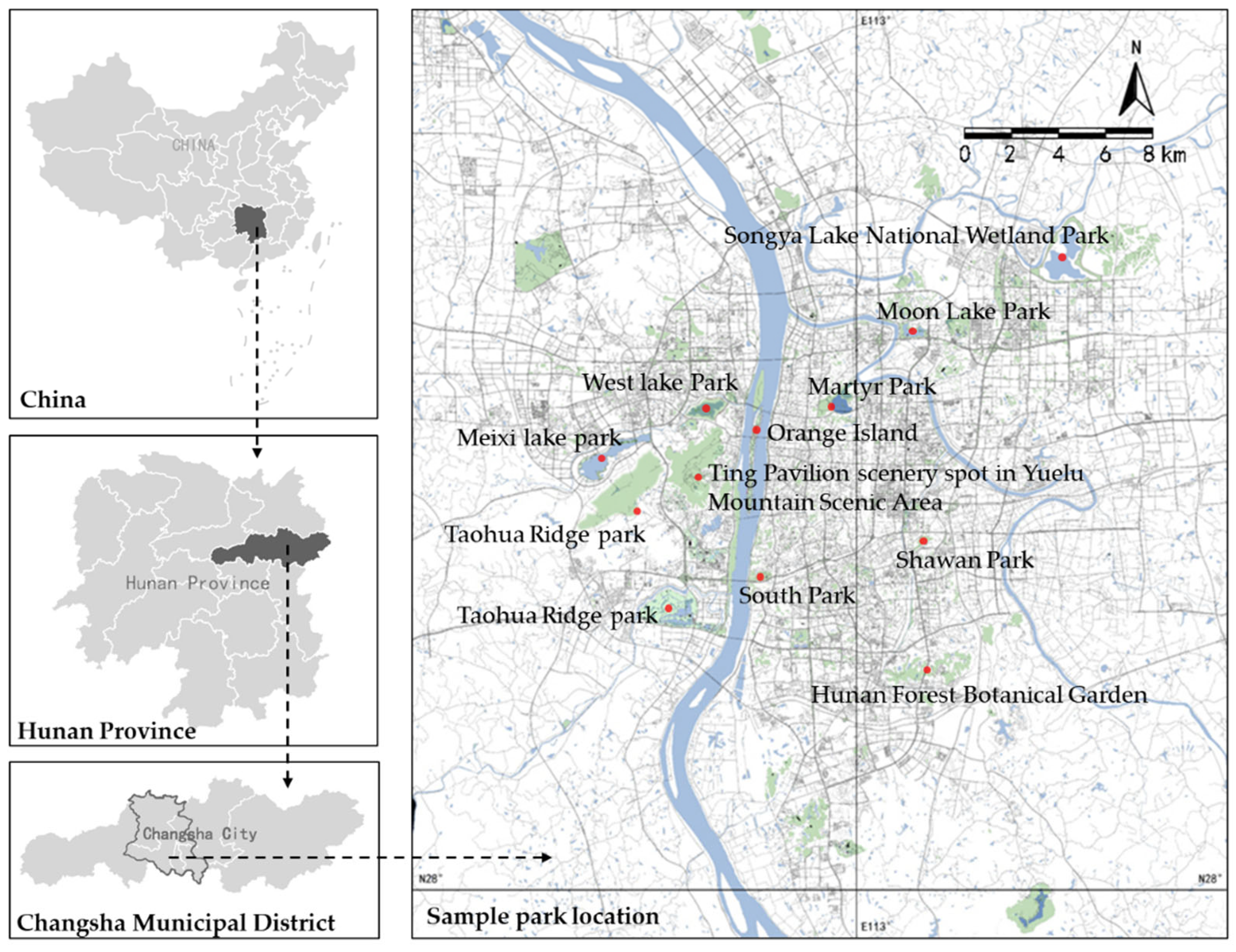
2.1. Study Area and Sample Plot Selection

Hunan Province is a provincial-level administrative region of China, bounded by latitude 24°38′–30°08′ north and longitude 108°47′–114°15′ east, with a total area of 21,800 square kilometers and a subtropical monsoon climate. Changsha is the capital city of Hunan Province.

As of 2020, there are 44 completed parks in Changsha (data from Changsha City Bureau of Statistics, http://tjj.changsha.gov.cn/, accessed on 20 October 2021). The main urban parks among them were selected for preliminary basic information investigation, and 12 parks were selected for the study based on completion time, scale, maintenance, geographic location and so on (Figure 1). These 12 parks were the main parks in the city’s neighborhoods with good public familiarity and high recognition. They were created between 1951–2016 and are of different sizes. These parks were well-maintained green spaces and had high quality plant landscapes. The specific information is shown in

Table 1. Basic information about the 12 parks surveyed.

Serial Number	Park Name	Park Location	Park Size (Hectares)	Number of Plant Communities Photographed	Number of plant Communities Selected
1	Orange Island	112°96′87.43″ N, 28°19′29.29″ E	91.6	62	6
2	Aiwan Ting Pavilion scenery spot in Yuelu Mountain Scenic Area	112°94′40.7″ N, 28°18′67.42″ E	0.6	55	7
3	West Lake Park	112°94′11.17″ N, 28°20′95.62″ E	148.1	123	23
4	Meixi Lake Park	112.90′90.83″ N, 28.19′89.34″ E	24.5	52	7
5	Taohua Ridge Park	112.90′66.28″ N, 28.18′16.04″ E	290.7	33	1
6	Yanghu Wetland Park	112.93′41.81″ N, 28.13′24.15″ E	485.0	82	10
7	Martyr Park	113.00′54.41″ N, 28.21′77.85″ E	153.3	127	17
8	Moon Lake Park	113.03′77.86″ N, 28.24′43.63″ E	66.9	30	3
9	South Park	112.97′21.74″ N, 28.14′67.3″ E	36.5	34	1
10	Shawan Park	113.04′56.6″ N, 28.16′12.36″ E	28.9	24	1
11	Hunan Forest Botanical Garden	113.03′84.55″ N, 28.10′95.94″ E	140.0	30	4
12	Songya Lake National Wetland Park	113.11′34.73″ N, 28.27′28.22″ E	365.0	69	5

.

2.2. Photography

Based on color science research, the most effective strategy at present is to use photosensitive shooting equipment to record the color picture of the real environment and conduct qualitative and quantitative evaluation and analysis of color [36]. A previous study showed that ambient lighting and time of day had an impact on color perception [32]. During the day, 10:00–16:00 was the best time to investigate landscape color [36]. The survey was conducted between 10:00 and 16:00 on a sunny day from November to December 2021. The same camera (Nikon D7200, Tokyo, Japan) was used by the same photographer to take smooth light shots. The camera was held upright, with the lens at eye height, and all shots were taken horizontally without a flash. A total of 721 photos were taken. Photos were screened according to the following principles: (1) The community contained colored foliage plants other than green that were in a stable stage of color change. (2) There were large trees in the community. (3) It was ensured that there was moderate light, and photos where the sky was too gray or too white were removed. (4) Nonplant elements in the foreground and middle-ground were avoided. (5) The plants in the community were all growing robustly, and there were no diseased or insect-infested species or stunted trees. A total of 85 photographs were obtained as the study sample after screening (Table 1).

2.3. Scenic Beauty Estimation

In this study, the scenic beauty estimation (SBE) was used to evaluate the color landscape beauty of autumn plant communities in parks in Changsha. Different types of evaluators generally had consistent aesthetic evaluations, and there was no significant difference between on-site and indoor evaluations [39]. An online questionnaire was used for photo presentation. All 85 photos were shown to each assessor and all photos were randomly ordered. Each photo was displayed only once and stayed on the display page for only 7 s. A 7-point scale was used to judge the degree of liking for the photos, and the scores were −3, −2, −1, 0, 1, 2 and 3, representing a rang from “not beautiful at all” to “most beautiful” [26]. Questionnaires were distributed through the online platform (https://www.wjx.cn/, accessed on 11 July 2022) to collect the results of the public’s scenic beauty evaluation of the sample plots. A total of 324 questionnaires were collected, and 297 valid questionnaires were obtained, accounting for 91.7%. SPSS26.0 was applied to test the overall reliability of the 297 questionnaires, and their Cronbach’s alpha coefficient was 0.982, indicating that the questionnaire had high reliability.

Table 2. Basic demographics of questionnaire subjects.

Basic Information	Category	Number	Percent (%)	Basic Information	Category	Number	Percent (%)
Ability to accurately identify colors	Yes	297	100	Education	Undergraduate	160	53.9
	No	0	0		Master’s degree	82	27.6
Gender	Men	132	44.4		PhD candidate	19	6.4
	Women	165	55.6	Annual park recreation times	0	5	1.7
Age	Under 18 years old	4	1.3		1~3	85	28.6
	18~25 years old	150	50.5		4~10	101	34.0
	26~30 years old	45	15.2		11~20	61	20.5
	31~40 years old	76	25.6		21~100	39	13.1
	41~50 years old	12	4.1		101~200	0	0
	51~60 years old	6	2.0		201 or more	6	2.0
	61 years old or older	4	1.3	Professional/occupation	Landscape architecture and related	137	46.1
Education	Primary education	18	6.1		Others	160	53.9
	Junior education	18	6.1

shows the basic demographics of the subjects.

The SBE value was calculated according to a previous method [40]. First, the frequency (f) of each grade was counted, and then the downward cumulative probability (p) of the corresponding grade was calculated. The one-sided quantile (z) was calculated from the standard normal distribution numerical table. Since the p value of the lowest rank value in the accumulation process must be 1 and $z=+\infty$, the z values except for the lowest grade value were used to calculate the average z ($\overline{z}$). When p = 1 or p = 0 in the other grades, $p=1-1/\left(2N\right)$ or $p=1/\left(2N\right)$ was used to approximate the z value, where N was the number of participants in the test. Therefore, the SBE value of the beauty value of the ith photo was

$$SB{E}_i=\left({\overline{z}}_i-{\overline{z}}_0\right)\times 100$$

(1)

${\overline{z}}_i$ is the average value of the unilateral quantiles of the ith picture. Any photo was chosen as the control photo. The SBE value of this photo was 0 and the mean value of its one-sided quantile z was ${\overline{z}}_0$.

The beauty value was divided into 5 grades by the Equation (2) [34]: Grade I (very beautiful), Grade II (beautiful), Grade III (general), Grade IV (ugly) and Grade V (very ugly).

$$X_i=\left[\left(SB{E}_{max}-SB{E}_{min}\right)\left(A_i-20\%\right)+SB{E}_{min}, \left(SB{E}_{max}-SB{E}_{min}\right)A_i+SB{E}_{min}\right]$$

(2)

$X_i$ was the level of the beauty value, $i$ was the value of I, II, III, IV and V. $A_I=100\%, A_{II}=80\%, A_{III}=60\%, A_{IV}=40\%, A_V=20\%.$ $SB{E}_{max}$ was the maximum beauty value, $SB{E}_{min}$ was the minimum beauty value.

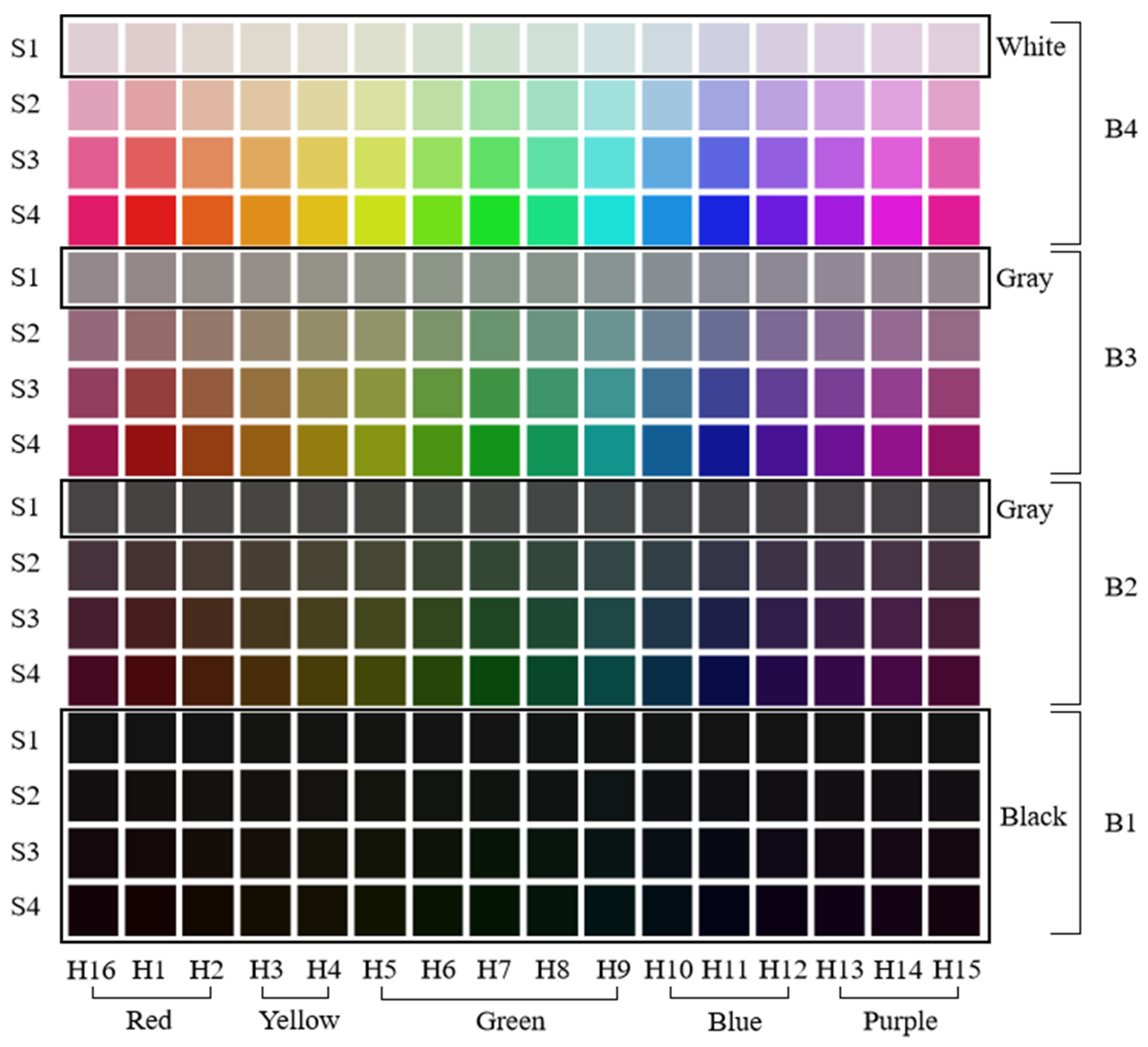
2.4. Color Quantization Based on the HSB Model

Choosing the appropriate color model is the premise of color quantization. The color model mainly includes CMYK, RGB, HIS, HSB, LAB, CHL, etc. [41]. The CMYK and RGB models are hardware-oriented, while the HSB model is user-oriented [42]. The HSB color model is close to the human eye’s color perception ability, and its advantage lies in the operation and expression of image color display, which can complete the quantization process in photography equipment and image display equipment [36]. In addition, in the HSB color model, the distance between two color points in space could be calculated by the Euclidean distance, which was conducive to extracting the quantitative color consistent with human discrimination ability [43]. Therefore, this study selected the HSB color model to investigate the color landscape of autumn plant communities.

The color value of the photos was extracted by Adobe Photoshop and ColorImpact. We selected the sky in Photoshop and filled it uniformly to facilitate color extraction. To establish a color database, the processed photos were imported into ColorImpact to extract the color HSB value and pixel ratio. Among them, only the color value of the sky pixel proportion was not calculated and analyzed. In addition, when the pixel proportion was too small, colors were difficult for humans to recognize; therefore, colors with pixel proportions <1% were not included in the data extraction and analysis.

It was complicated to describe colors directly by the HSB value. To facilitate quantification, H, S and B were usually divided into different categories to reduce the number of colors. At present, an image retrieval algorithm based on the HSB model in the computer field is often used for reference. The H, S and B values of the images were nonuniformly quantified according to the empirical value of color perception of the human visual system [10,11,13,18,26]. Zhang extracted 75 colors in her study [11], Smith extracted 166 colors [44], Ma, Shi et al. extracted 256 colors [13,18] and Zhang, Mu et al. extracted 147 colors [10,26]. Too many colors could increase the difficulty of calculation, and too fine a color division may exceed the recognition ability of human eyes. If the number of colors is too small, much color information will be lost. According to Tian’s method [45], this paper carried out nonuniform quantization processing on colors, divided the H-value into 16 intervals, divided the S-value and B-value into 4 intervals, and obtained 256 colors. Then, according to Zhang and Mu’s method, the color values with too low saturation and brightness were normalized to white, gray and black, and 147 colors were ultimately obtained with 144 colors plus black, white, and gray. On this basis, 147 colors were classified according to hue. H1, H2 and H16 were red; H3 and H4 were yellow; H5, H6, H7, H8 and H9 were green; H10, H11 and H12 were blue; and H13, H14 and H15 were purple (Figure 2).

2.5. Selection of Color Element Indicators

The color element indicators were selected based on the following principles: first, indicators and research conclusions were selected from studies on forest color landscape and plant community color landscape; second, experts in the landscape industry were consulted; and third, indicators were adjusted and selected according to the actual situation of this study.

The indicators for the quantitative study of forest color landscapes and plant community color landscapes could be classified into two color property indicators: hue-, saturation- and brightness-related indicators and color composition relationship indicators, including color number, color diversity index, color uniformity index, color harmony relationship index and color layout relationship index, etc. In addition, the quantitative indicators of forest color landscape also included indicators related to color spatial pattern, such as patch shape, patch pattern, patch shape index, and aggregation index. The research scale of the plant color landscape determined the focus of this research. Forest color landscape studies have given more attention to the spatial pattern of color. Plant community color landscape studies have given more attention to the relationship between color compositions.

Previous studies on the color landscape of autumn plant communities have shown that color diversity [11,13,17,46], color uniformity [10,11,13,14,26], hue and its related factors [10,11,12,13,14,18,26,31,36], warm and cold colors and their proportions [13,17], color layout and other factors are highly correlated with the aesthetic quality of the plant color landscape. Moreover, among the color properties, the influence of hue-related factors on scenic beauty is higher than that of saturation and brightness [12,31]. On this basis, combining the opinions of experts in the field and the actual situation of this study, two types of indicators were selected: color properties and color composition relationship (

Table 3. Quantitative indicators of color elements.

Element	Indictor	Abbreviation	Formula
Color properties	Hue Index	IH	$I_H={\displaystyle \sum }_{i=1}^n\left(H_i\times R_{Hi}\right)$; $H_i$ is the i’th hue value, and $R_{Hi}$ is the proportion of pixels occupied by the i’th hue. I = 1, 2,…, 16.
	Saturation Index	IS	$I_S={\displaystyle \sum }_{i=1}^n\left(S_i\times R_{Si}\right)$; $S_i$ is the i’th saturation value, and $R_{Si}$ is the pixel proportion of the i’th saturation, i = 1,2,…, 4.
	Brightness Index	IB	$I_B={\displaystyle \sum }_{i=1}^n\left(B_i\times R_{Bi}\right)$; $B_i$ is the i’th brightness value, and $R_{Bi}$ is the proportion of pixels occupied by the i’th brightness, i = 1, 2,…, 4.
Color Composition Relation	Number of Color	NC	NC = SUM (HaSbBc), HaSbBcPi ≥ 1%; the number of colors whose pixel ratio is ≥1% among 147 colors. Pi is the pixel proportion of the ith color.
	Color Diversity Index	HC	$H_C=-{\displaystyle \sum }_{i=1}^s\left(P_i\times \ln P_i\right); P_i$ is the pixel proportion of the i’th color, and S is the number of colors, $S=N_C$.
	Color Evenness Index	EC	EC = HC/lnS; HC is color diversity index, and S is color number, $S=N_C$.
	Number of Primary Color	NP	In red, yellow, green, blue and purple, the number of colors with 40~100% pixels.
	Ratio of Primary Color	RP	In red, yellow, green, blue and purple, the proportion of pixels in the color system is 40~100%.
	Number of Adjunctive Color	NA	In red, yellow, green, blue and purple, the number of colors with 10~40% pixels.
	Ratio of Adjunctive Color	RA	In red, yellow, green, blue and purple, the proportion of pixels in the color system is 10~40%.
	Number of Intersperse Color	NI	In red, yellow, green, blue and purple, the number of colors <10% pixels.
	Ratio of Intersperse Color	RI	In red, yellow, green, blue and purple, the proportion of pixels in the color system is <10% pixels.
	Ratio of Primary Hue	RPH	In addition to black, white and gray, the pixel proportion of the largest hue.
	Color-Leafed Index	RC	$R_C=P_{H1}+P_{H2}+P_{H3}+P_{H4}+P_{H16};$ $P_{H1,}$ $P_{H2}$, $P_{H3}$, $P_{H4}$ and $P_{H16}$ are the pixel proportions of hue H1, H2, H3, H4 and H16, respectively.
	Ratio of Warm and Cool Color	RWC	$R_{WC}=S_W/S_C;$ $S_W$ is the warm-tone pixel, $S_C$ is the cold-tone pixel.

Note: (1) The division of primary color, adjunctive color and intersperse color involved in N_P, R_P, N_A, R_A, N_I, R_I: according to the proportion of area, the color proportion was 40~100% for the primary color, 10~40% for the adjunctive color, and 0~10% for the intersperse color [10,47]. (2) The division of warm and cold colors in R_WC: In the five color systems, red and yellow are warm colors, and green, blue and purple are cool colors.

).

2.6. Data Processing and Analysis

SPSS26.0 and Microsoft Office Excel were mainly used for data processing, analysis and chart drawing.

2.6.1. Analysis of the Relationship between the Structural Characteristics of Plant Communities and the SBE Values

In addition to color, the composition characteristics of the plant community may also have an impact on the SBE value. The 85 sample plots were classified on the basis of two factors: the number of plant varieties and the vertical structure level of the plant community. Based on the number of plant varieties in the community, the sample plots were classified into three types: simple varieties (NV1), moderate varieties (NV2), and complex varieties (NV3). NV1 was a sample plot containing 1–3 plant varieties in the community, with 20 sample plots; NV2 was a sample plot containing 4–6 plant varieties in the community, with 51 sample plots; and NV3 was a sample plot containing 7 or more plant varieties in the community, with 14 sample plots. The sample plots were divided into three types according to the vertical structure of the plant community: 2-layer structure community (PL1), 3-layer structure community (PL2), and 4-layer and above structure community (PL3). The 2-layer structure community consisted of trees + shrubs, trees + herbaceous flowers, and trees + grass, with 27 sample plots; and the 3-layer structure community was a combination of trees + shrubs + ground cover, with 35 sample plots. The 4-layer and multilayer plant communities were in the form of trees + shrubs + ground cover + herbaceous flowers or grasses, with a total of 23 sample plots. One-way ANOVA and multiple comparison analysis were used to analyze the differences between groups in the SBE values of NV1, NV2 and NV3 and the differences between groups in the SBE values of PL1, PL2 and PL3 to explore the influence of two factors, the number of varieties and the vertical structure level of the plant community, on the SBE values.

2.6.2. Construction of Color Landscape Characteristic Index and Comprehensive Model of Autumn Plant Community in Urban Parks

The color element indicators are intertwined, affect each other and are numerous. To avoid the problems of multiple collinear relationships and large errors in regression prediction results, this study used principal component analysis to reduce the dimensionality of the original indicators and form a new variable group that was independent of each other and contained the information of the original variables and then established the plant color landscape characteristic indices and comprehensive model.

The following steps were included: (1) 85 groups of data of 15 original color element indicators were input into SPSS26.0, the Z score was selected for standardization, and then PCA (principal component analysis) was conducted to extract the principal components with a characteristic value >1. (2) The relationship between each principal component and the original color element indicators was determined based on the rotation matrix, and it was named. (3) Based on the factor load coefficient and eigenvalue of the color element indicator, its coefficient in the linear combination of each principal component was calculated from Equation (3), and the initial weight of each color element indicator was obtained from Equation (4). After standardization, the contribution degree of each color element indicator to the quality of the autumn color landscape was obtained. (4) According to the total variance interpretation, the weight of each principal component was calculated from Equation (5), and a comprehensive model of autumn plant color landscape quality was constructed.

$$a_{ij}=\frac{{\mu }_{ij}}{\sqrt{{\lambda }_j}}\left(i=1,2,3,\dots ,m;j=1,2,3,\dots ,n\right)$$

(3)

$a_{ij}$ is the coefficient of the i’th indictor in the j’th principal component linear combination, ${\mu }_{ij}$ is the factor loading coefficient of the j’th principal component of the i’th variable, ${\lambda }_j$ is the characteristic root represented by the j’th principal component.

$$w_i\prime =\frac{a_{i1}\times {\theta }_1+a_{i2}\times {\theta }_2+a_{i3}\times {\theta }_3+\dots +a_{ij}\times {\theta }_j}{{{\displaystyle \sum }}_j^n{\theta }_j}$$

(4)

$w_i\prime$ is the initial weight of the i’th indicator, $a_{ij}$ is the coefficient of the i’th indictor in the j’th principal component linear combination, ${\theta }_1$ is the variance contribution rate corresponding to the j’th principal component.

$${\mathrm{Q}}_{\mathrm{n}}=\frac{P_{var}}{R_{var}}$$

(5)

$P_{var}$ is the percentage of variance, and $R_{var}$ is the cumulative contribution rate of variance.

2.6.3. Correlation Analysis between Color Landscape Characteristic Indicators and SBE Grades of the Plant Community

One-way analysis of variance (ANOVA) was performed on the plant color landscape characteristic indices to obtain their significant differences among different SBE grades. If there were highly significant or significant differences, they were analyzed by least significant difference (LSD) for multiple comparisons analysis. At the same time, the results of the one-way ANOVA of the original color element indicators were also combined. The correlations between plant color landscape characteristic indices and color element indicators and SBE grades were further explored.

2.6.4. Classification of Color Composition Types of Plots with a High SBE Level (Grade I and II)

Q-type clustering was used to classify the sample plots of high SBE level (Grade I and II) by intragroup links and square Euclidean distance, and the color composition characteristics of each type were analyzed. To explore the intrinsic properties and composition rules of plant color landscapes with high SBE values, the top three sample plots with SBE values in each type were selected for quantitative analysis of color composition.

3. Results

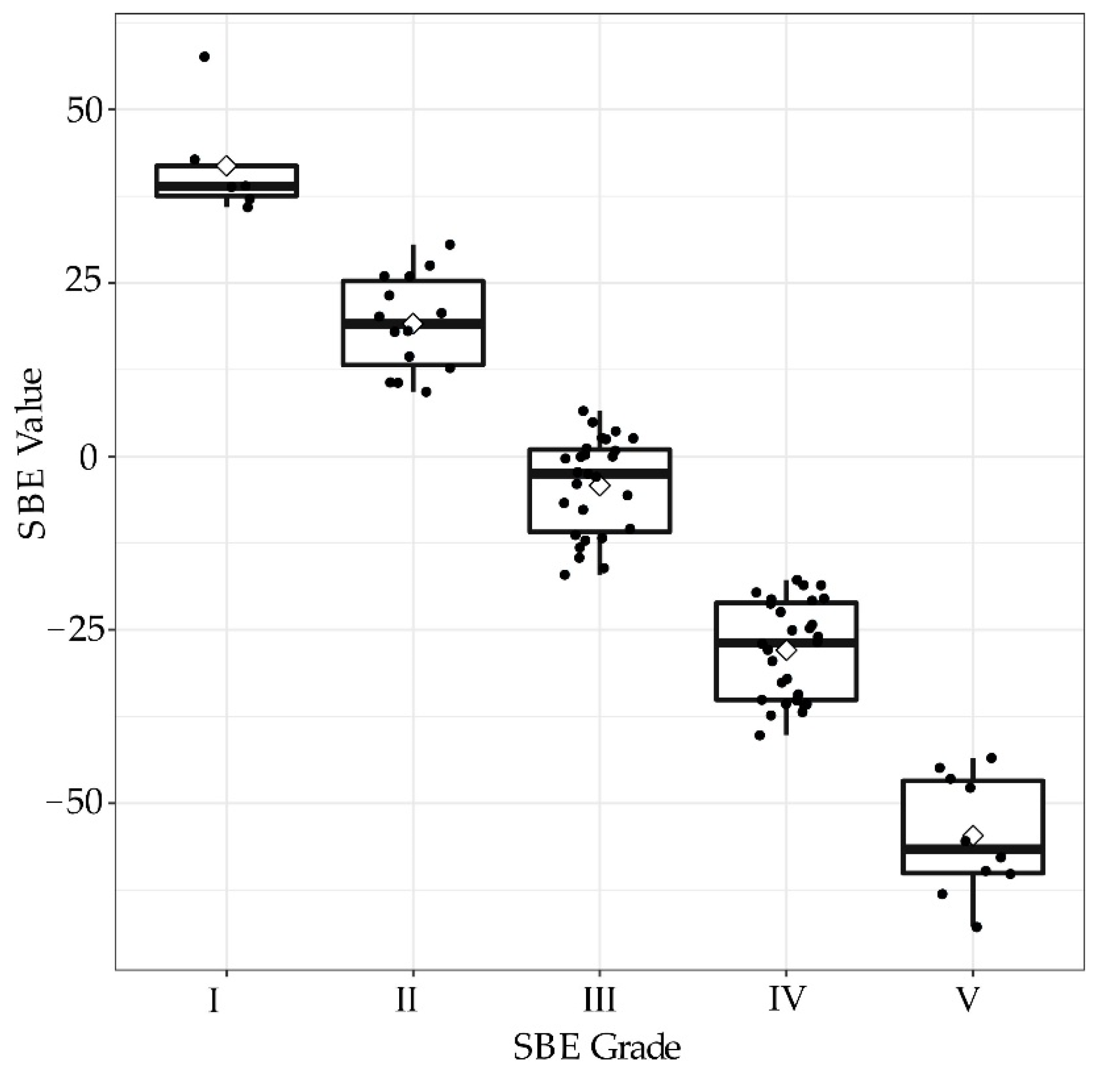
3.1. Landscape Beauty Evaluation

The results of multivariate repeated measurement ANOVA showed that the SBE value was p < 0.001, indicating that the difference in the SBE value in each location was statistically significant. The SBE values of 85 plots ranged from 57.60 to −67.84, with 6 of Grade I (very beautiful), 14 of Grade II (beautiful), 27 of Grade III (general), 28 of Grade IV (ugly) and 10 of Grade V (very ugly). The corresponding SBE values of Grades I, II, III, IV and V were (32.51, 57.60), (7.42, 32.51), (−17.66, 7.42), (−42.75, −17.66), and (−67.84, −42.75), respectively. Overall, 55.3% of plots were in Grades I, II and III, and only 23.5% of plots were in Grades I and II (Figure 3), which indicated that the evaluation of autumn plant landscape color in the Changsha city park was at an average level, but some plant landscapes were still recognized by the public, and the overall quality of the plant color landscape needed to be improved.

3.2. Relationship between the Structural Characteristics of Plant Communities and the SBE Values

The results of one-way ANOVA and multiple comparison analysis showed that there were no significant differences in the SBE values between the NV1 (simple varieties), NV2 (moderate varieties), and NV3 (complex varieties) groups with different numbers of plant varieties (p = 0.611). There were no significant differences in the SBE values between NV1 and NV2 (p = 0.347), NV1 and NV3 (p = 0.439), and NV2 and NV3 (p = 0.944). There were also no significant differences in the SBE values between the PL1 (2-layer structure community), PL2 (3-layer structure community) and PL3 (4-layer and above structure community) groups at different levels of community vertical structure (p = 0.829). There were no significant differences in the SBE values between PL1 and PL2 (p = 0.680), PL1 and PL3 (p = 0.739), and PL2 and PL3 (p = 0.968). It can be concluded that the basic compositional characteristics of the plant community did not have a significant effect on the color beauty in this study. It can also be concluded that the number of plant varieties and vertical structure level, the two basic compositional characteristics of the community, did not have a significant effect on the SBE values in this study.

3.3. Construction of the Color Landscape Characteristic Index and Comprehensive Model of Autumn Plant Community in Urban Parks

The results of the PCA (principal component analysis) (Table S1) showed that the Kaiser–Meyer–Olkin (KMO) index was 0.673, which was significantly greater than 0.5, while Bartlett’s sphericity test probability p value was 0.000 < 0.01, showing that the sample data were determined to be suitable for PCA [26,48,49]. The four principal components with eigenvalues greater than 1 were extracted, and the explanatory variances were 36.087%, 20.096%, 14.878%, and 10.036%, respectively, with a cumulative value of 81.097% (Table S2), indicating that these four principal components could explain 81.097% of the information of 15 indicators, and the data were valid. Therefore, these four principal components were extracted for subsequent analysis.

The principal components were extracted based on the rotated matrix (Table S3). The first principal component (PC1) was loaded more on the ratio and number of primary colors, ratio of the primary hue, and ratio and number of adjunctive colors. These indicators mainly reflected the primary and adjunctive color situation of plant communities; therefore, PC1 was defined as the primary and adjunctive color index. The second principal component (PC2) was loaded more on the color uniformity index, brightness index, color diversity index, saturation index, color number and hue index. These indicators mainly reflected the structural and property characteristics of plant colors. Therefore, PC2 was defined as the color structure and property index. The third principal component (PC3) was loaded more on the ratio of warm and cold colors and color-leafed index, which reflected the discoloration of plants in autumn. Therefore, PC3 was defined as the autumn color-leafed index. The fourth principal component (PC4) was loaded more on the ratio and number of intersperse colors, which mainly reflected the interspersed color situation of the plant communities; therefore, PC4 was defined as the intersperse color index.

The coefficients of each color element indicator in the linear combination of principal components were calculated by Equation (3) (

Table 4. Coefficients of color element indicators in linear combinations of different principal components.

Serial Number	Color Element Indicator	Component
		1	2	3	4
1	RP (Ratio of Primary Color)	0.413	0.074	0.000	−0.128
2	NP (Number of Primary Color)	0.388	0.058	−0.006	−0.168
3	RPH (Ratio of Primary Hue)	0.358	0.005	0.037	−0.110
4	RA (Ratio of Adjunctive Color)	−0.353	0.190	−0.030	−0.160
5	NA (Number of Adjunctive Color)	−0.339	0.202	−0.081	−0.154
6	EC (Color Evenness Index)	−0.146	0.494	−0.034	−0.020
7	IB (Brightness Index)	0.034	0.487	−0.009	0.051
8	HC (Color Diversity Index)	−0.186	0.470	−0.137	0.118
9	IS (Saturation Index)	0.108	0.393	0.145	−0.122
10	NC (Number of colors)	−0.204	0.346	−0.226	0.271
11	RWC (Ratio of Warm and Cool Color)	0.052	−0.043	0.559	−0.159
12	RC (Colored Index)	0.057	0.249	0.533	−0.087
13	IH (Hue Index)	−0.010	0.225	−0.501	−0.039
14	RI (Ratio of Intersperse Color)	−0.023	0.034	−0.131	0.750
15	NI (Number of Intersperse Color)	−0.084	0.000	−0.030	0.746

), and four comprehensive indices of color landscape quality of plant communities in autumn are as follows:

PC1 = 0.413R_P + 0.388N_P + 0.358R_PH + … − 0.023R_I − 0.084N_I

PC2 = 0.074R_P + 0.058N_P + 0.005R_PH + … + 0.034R_I + 0.000N_I

PC3 = 0.000R_P − 0.006N_P + 0.037R_PH + … − 0.131R_I − 0.030N_I

PC4 = −0.128R_P − 0.168N_P − 0.110R_PH + … + 0.750R_I + 0.746N_I

After obtaining the weights of each color element index by Equation (4) and normalizing them, their contribution to the color landscape quality of the autumn plant community was obtained (Figure 4). The weights of the four color landscape quality indices were calculated by Equation (5): Q1 = 0.445, Q2 = 0.248, Q3 = 0.183, Q4 = 0.124, and Y (comprehensive color landscape quality of the autumn plant community) = 0.445PC1 + 0.248PC2 + 0.183PC3 + 0.124PC4.

3.4. Correlation between the Color Landscape Characteristic Index and SBE Grade of the Autumn Plant Community

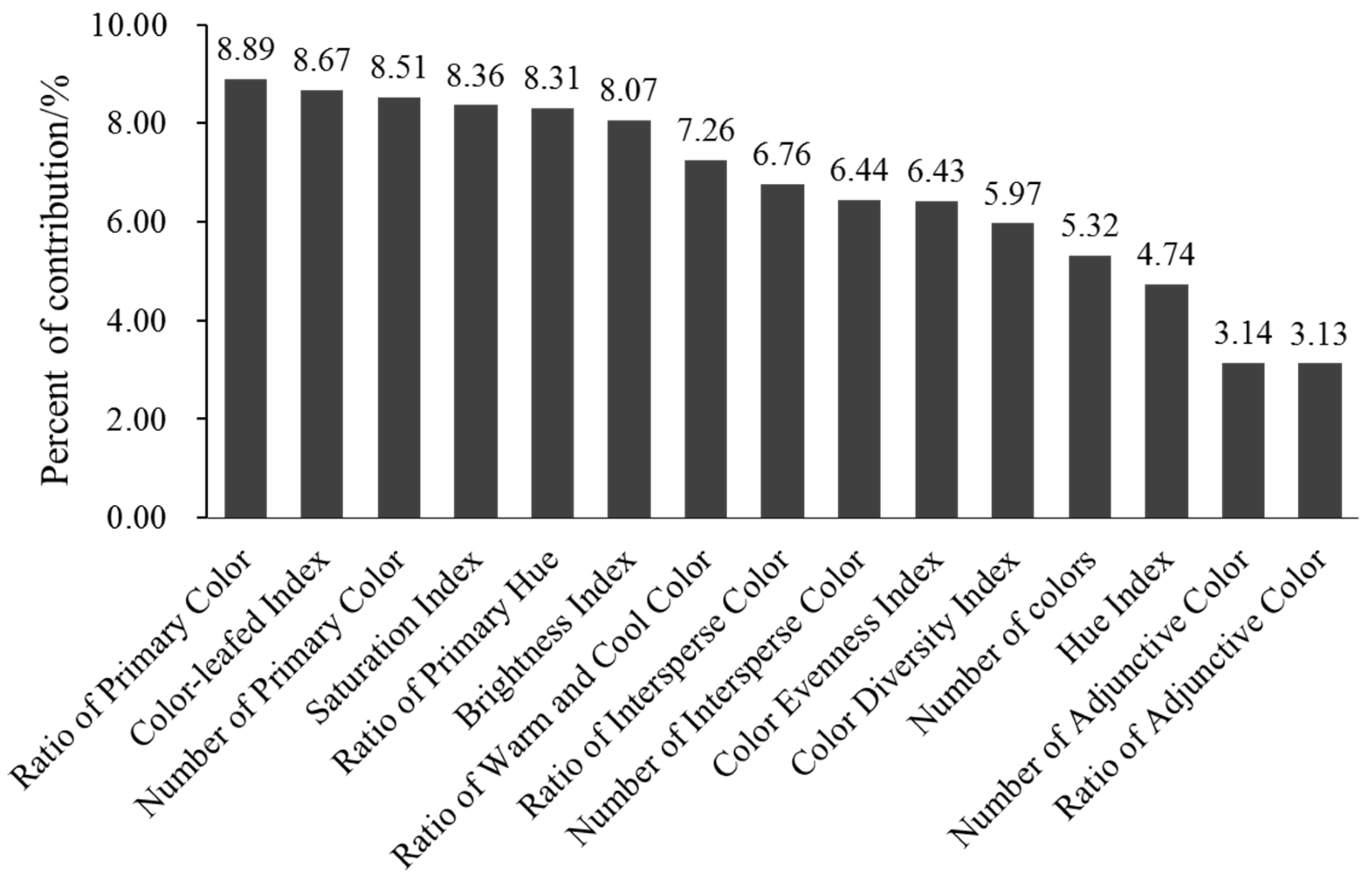
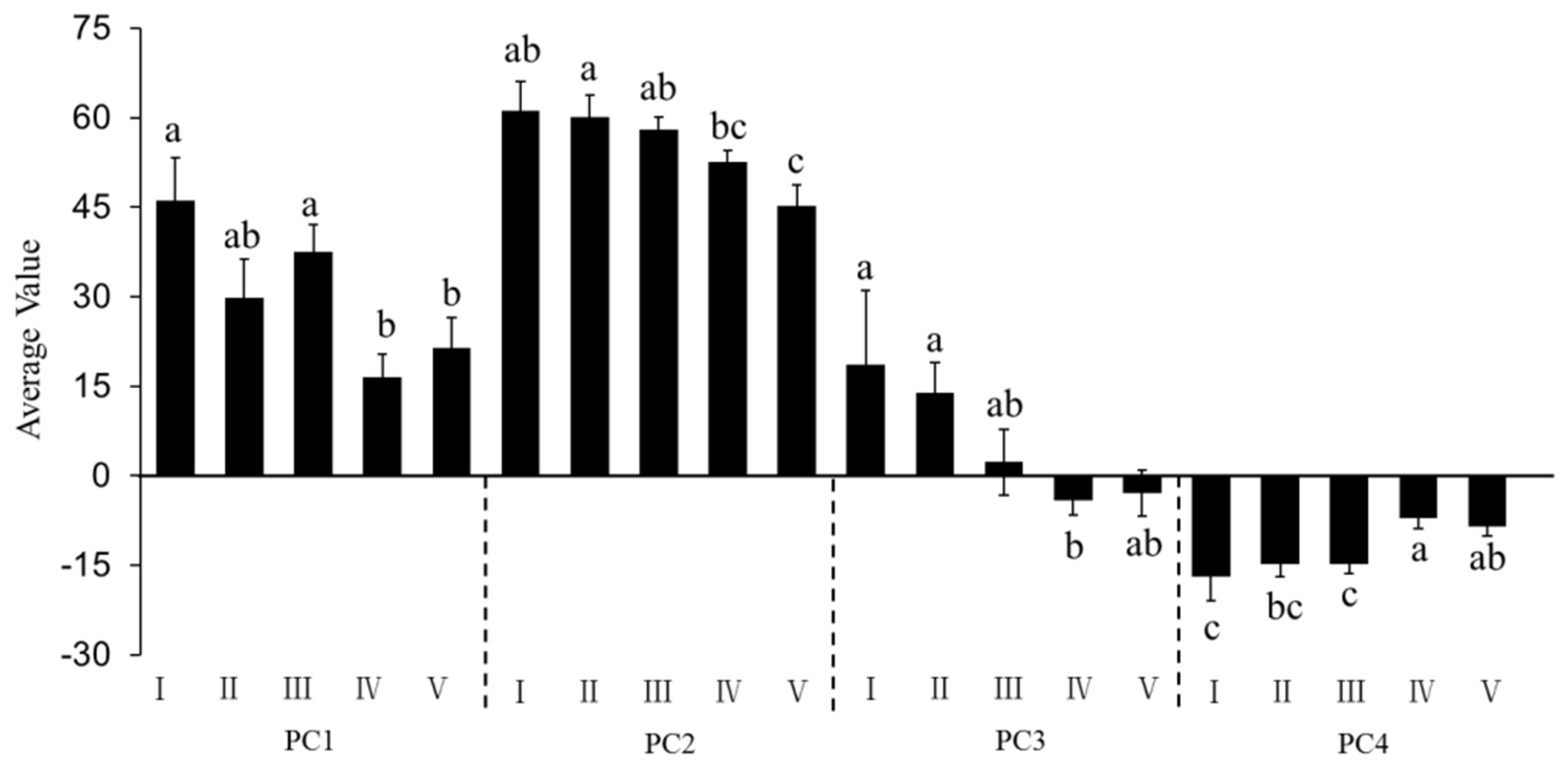
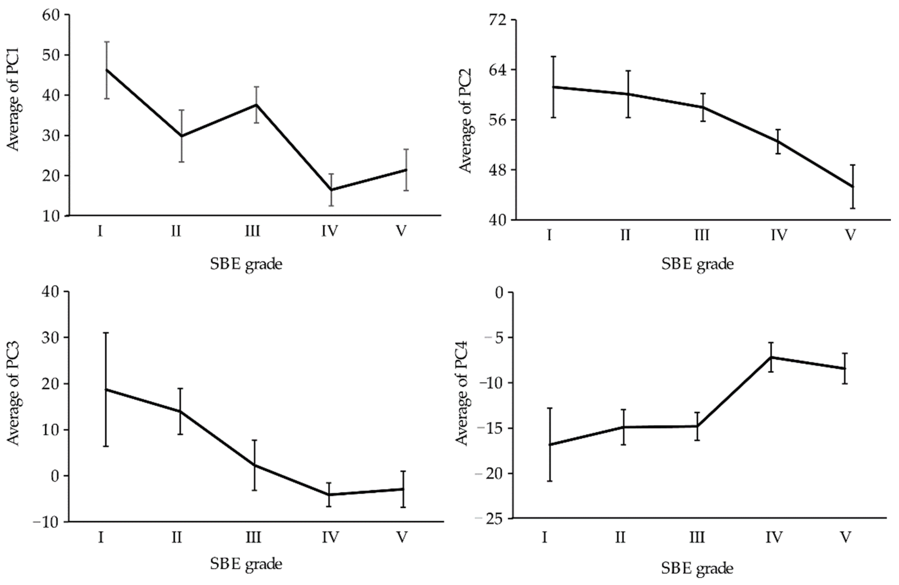
3.4.1. The Effect of Principal Components on SBE Grade

The results of one-way ANOVA (Table S4) showed that the differences were highly significant for PC1 (primary and adjunctive color index) (p = 0.002), PC2 (color structure and property index) (p = 0.008) and PC4 (intersperse color index) (p = 0.001) and significant for PC3 (autumn color-leafed index) (p = 0.036) among the five SBE grades. To further distinguish between which beauty grades the four color landscape quality indices differentiated, multiple comparisons were made using the LSD method. The results (Figure 5) showed that PC1 was highly significantly different between Grades I and IV and III and IV and significantly different between Grades I and V and III and V. PC2 was highly significantly different between Grades I, II, III and V and significantly different between Grades II and IV. PC3 was significantly different between Grades I and IV and Grades II and IV. PC4 was highly significantly different between Grades I, II, III and IV and significantly different between Grades I and V and between Grades III and V. Overall, there were no significant differences in the four comprehensive indices between Grades I and II and between Grades IV and V, while there were at least one and up to three comprehensive indices between Grades I and II and Grades IV and V that had significant or extremely significant differences. Therefore, the five SBE grades can be integrated into three levels: high SBE level (Grades I and II), medium SBE level (Grade III), and low SBE level (Grades IV and V).

The figure of the mean values of the four principal components (Figure 6) indicated that the mean value of PC1 showed an overall decreasing trend as the SBE grade decreased, although there was a slight increase in Grades III and V. The values of PC1 were much higher in the high SBE level samples than in the low SBE level samples. The mean value of PC2 decreased with decreasing SBE grades. The two showed a significant positive correlation. The mean value of PC3 decreased with decreasing SBE grades and only slightly increased in Grade V. The two showed a significant positive correlation in general. The mean value of PC4 increased with decreasing SBE grades and only slightly decreased in Grade V. The two showed a significant negative correlation in general.

3.4.2. Correlation between Color Element Indicators and SBE Grades

The results of one-way ANOVA of 15 original color element indicators showed that SBE grades were highly significantly correlated with R_PH (ratio of primary hue) (p = 0.001), R_P (ratio of primary color) (p = 0.002), and R_C (color-leafed index) (p = 0.004), and they were significantly correlated with R_WC (ratio of warm and cool color) (p = 0.013) and N_C (color-leafed index) (p = 0.027). Among these five indicators, there was a positive correlation with the SBE grades in general, except N_C was negatively correlated with the SBE grades. However, the mean value of N_C reached the highest level in Grade IV and decreased in Grade V. In addition, the brightness index and saturation index were positively correlated with SBE grade.

Combined with the changes in the original color element indicators among different grades (

Table 5. Variation range of color element indicator of each SBE grade.

Color Element Indicator	Mean ± SE
	I	II	III	IV	V
RPH (Ratio of Primary Hue)	51.16 ± 9.30 a	45.59 ± 4.20 a	49.56 ± 3.36 a	33.15 ± 2.38 b	34.59 ± 4.03 b
RWC (Ratio of Warm and Cool Color)	18.67 ± 6.97 a	7.32 ± 1.83 b	8.78 ± 2.37 b	4.01 ± 1.19 b	4.00 ± 1.49 b
RC (Color-leafed Index)	52.97 ± 10.90 a	50.50 ± 6.54 a	38.75 ± 5.12 ab	28.80 ± 2.44 b	25.02 ± 4.55 b
NP (Number of Primary Color)	1.00 ± 0.00 a	0.71 ± 0.13 ab	0.81 ± 0.08 a	0.54 ± 0.11 b	0.60 ± 0.16 ab
RP (Ratio of Primary Color)	56.83 ± 7.06 a	40.46 ± 7.68 ab	49.74 ± 4.99 a	24.68 ± 4.98 b	26.98 ± 7.38 b
NA (Number of Adjunctive Color)	0.33 ± 0.21 a	1.00 ± 0.26 a	0.63 ± 0.17 a	1.00 ± 0.18 a	0.70 ± 0.15 a
RA (Ratio of Adjunctive Color)	5.29 ± 3.55 a	22.79 ± 5.96 ab	13.77 ± 3.45 ab	22.62 ± 4.21 b	12.84 ± 3.52 ab
NI (Number of Intersperse Color)	1.83 ± 0.31 a	1.86 ± 0.33 a	1.59 ± 0.14 a	2.11 ± 0.21 a	1.60 ± 0.27 a
RI (Ratio of Intersperse Color)	6.85 ± 2.18 a	6.10 ± 1.11 a	6.04 ± 0.82 a	7.74 ± 0.98 a	4.59 ± 0.98 a
NC (Number of colors)	7.17 ± 0.70 b	7.79 ± 0.69 b	8.15 ± 0.46 b	9.71 ± 0.44 a	8.00 ± 0.71 a
HC (Color Diversity Index)	1.26 ± 0.14 ab	1.41 ± 0.12 ab	1.32 ± 0.07 b	1.53 ± 0.08 a	1.29 ± 0.11 ab
EC (Color Evenness Index)	0.64 ± 0.04 a	0.69 ± 0.03 a	0.63 ± 0.02 a	0.67 ± 0.02 a	0.62 ± 0.03 a
IH (Hue Index)	46.23 ± 6.79 ab	38.25 ± 3.39 b	51.13 ± 4.36 a	44.46 ± 2.22 ab	39.51 ± 4.07 ab
IS (Saturation Index)	31.74 ± 4.38 a	29.83 ± 1.90 a	28.69 ± 1.37 ab	26.81 ± 1.45 ab	23.22 ± 2.48 b
IB (Brightness Index)	34.39 ± 2.67 a	32.41 ± 2.46 a	31.28 ± 1.45 a	28.27 ± 1.13 ab	25.85 ± 2.04 b

Note: Different lowercase letters indicate significant differences between different grades (p < 0.05).

), the color composition characteristics of the three levels of SBE grade plots were analyzed. The color composition characteristics of the high SBE level plots (Grades I and II) were as follows: high ratio of primary hue, and high number and ratio of primary color; the ratio of warm and cold colors and color-leafed index were much higher than those in the Grade IV and V plots. The number and ratio of adjunctive colors were higher, the number of colors was low, and the saturation index and brightness index were high. The color characteristics of medium SBE level plots (Grade III) were as follows: high ratio of primary hue, but medium number and ratio of primary color; the number of intersperse color was low, hue index was high, and the other indicators were located in the middle grade. The color characteristics of the low SBE level (Grades IV and V) plots were as follows: the ratio of primary hue, primary color, warm and cold color, and the color-leafed index were much lower than those of the high SBE level (Grade I and II) plots. The number of colors was high, and the saturation index and brightness index were low. The ratio of adjunctive color and intersperse color in Grade V was low, indicating that the proportion of neutral color (black, white, and gray) was higher.

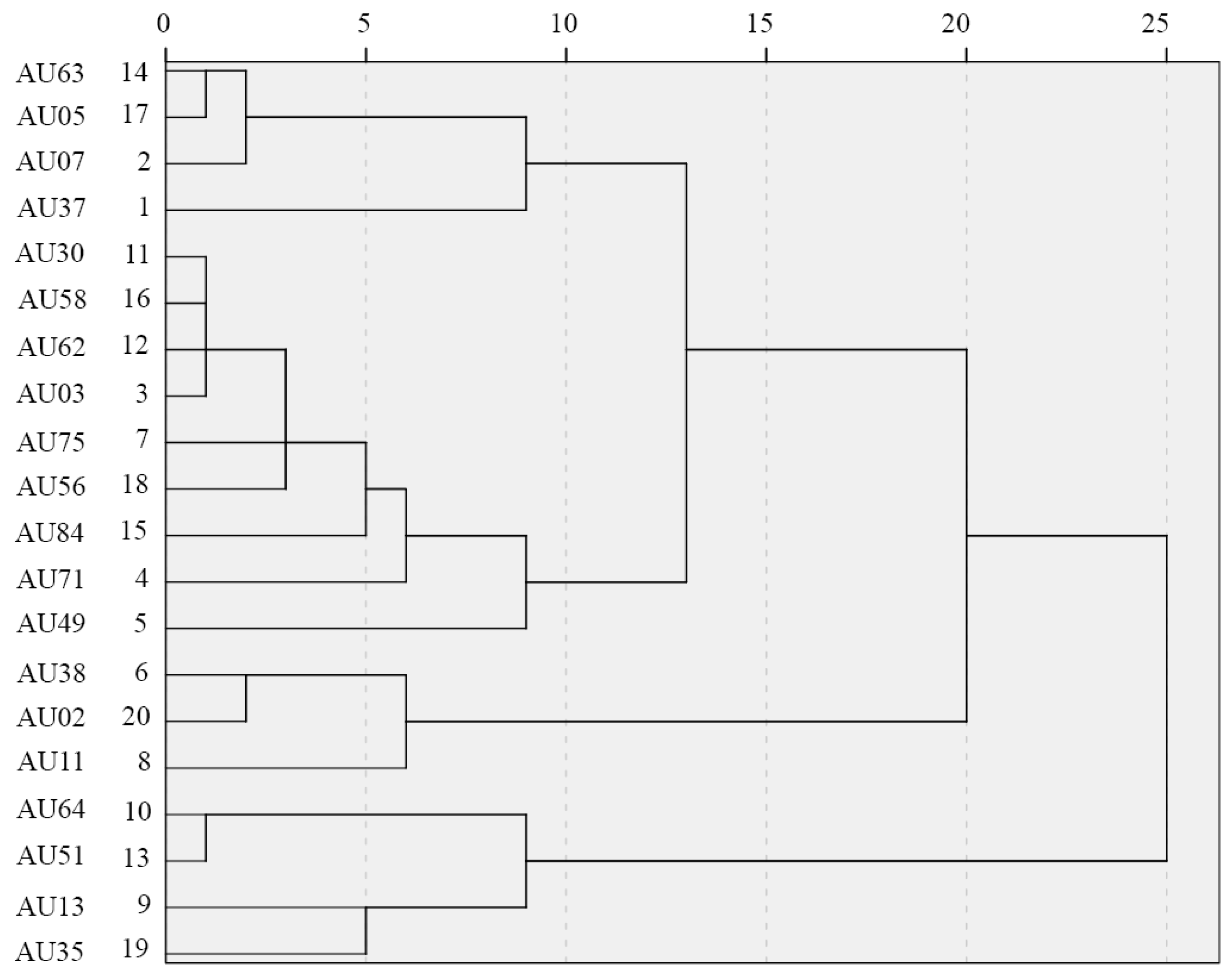
3.5. Classification and Color Composition Characteristics of Plots with High SBE Level (Grade I and II)

Based on four plant community color landscape characteristic indices, systematic cluster analysis was conducted on 20 sample plots of Grades I and II. The results can be used to determine the type of color composition of autumn plant communities with high SBE level. The intragroup differences were divided by square Euclidean distance for Q-type clustering. When the distance coefficient was selected as 15, 20 plots could be divided into three types. The first type, T1 (warm-toned dominant type), contained 13 plots, accounting for 65%, and the mean SBE value was 27.97. The second type, T2 (warm and cold-toned contrast type), contained 3 plots, accounting for 15%, and the mean SBE value was 24.24. The third type, T3 (multicolor harmonic type), contained 4 plots, accounting for 20%, and the mean SBE value was 20.68. Analysis of variance showed that PC1 (p < 0.001) and PC3 (p = 0.001) had extremely significant differences among these three types of sample plots, while PC2 (p = 0.086) and PC4 (p = 0.090) had no significant differences among the three types. These results indicated that the main differences among the three types of plots were primary hue, primary color, adjunctive color and autumn color-leafed related indicators.

3.6. Quantitative Color Analysis of High-Quality Plant Communities

The top three plots with SBE values in T1 (warm-toned dominant type), T2 (warm and cold-toned contrast type) and T3 (multicolor harmonic type) were selected for quantitative analysis to explore the intrinsic properties of the color composition of plant communities with high SBE values (

Table 6. Quantitative color analysis of high-quality plant communities.

Plot Type and Number	Sample Photos	Typical Constitutive Color	Color Property Values	Hue Category and Proportion %	Primary Color and Proportion %	Classification of the Number of Plant Varieties	Classification of Vertical Structure Levels	SBE Value
T1-AU37			H:14° S:31% B:16%	H1 21.96	Red 40.48	NV1	PL1	57.60
			H:23° S:62% B:32%	H2 12.15
			H:26° S:54% B:41%	H3 6.41
			H:23° S:47% B:58%	H2 6.37
			H:29° S:37% B:69%	H3 4.86
T1-AU07			H:39° S:63% B:31%	H3 27.43	Yellow 40.25%	NV1	PL2	42.81
			H:50° S:49% B:63%	H4 7.03
			H:30° S:57% B:58%	H3 5.79
			H:65° S:61% B:51%	H5 3.17
T1-AU03			H:37° S:45% B:30%	H3 48.88	Yellow 57.38	NV1	PL1	38.99
			H:24° S:46% B:57%	H2 9.32
			H:47° S:38% B:64%	H4 8.50
			H:67° S:49% B:51%	H5 3.18
T2-AU38			H:60° S:17% B:23%	H5 70.25	Green 73.84	NV2	PL2	35.92
			H:49° S:38% B:64%	H4 3.82
			H:39° S:38% B:53%	H3 3.73
			H:78° S:32% B:52%	H5 3.59
T2-AU11			H:60° S:25% B:22%	H5 44.84	Green 50.09	NV3	PL3	27.50
			H:53° S:40% B:64%	H4 5.64
			H:22° S:46% B:58%	H2 3.26
			H:71° S:58% B:52%	H5 2.29
			H:78° S:32% B:52%	H5 1.60
T2-AU02			H:71° S:46% B:18%	H5 68.30	Green 78.04	NV2	PL2	9.31
			H:66° S:41% B:63%	H5 5.83
			H:73° S:46% B:53%	H5 3.91
			H:13° S:41% B:58%	H1 3.59
T3-AU13			H:49° S:30% B:15%	H4 19.39	None	NV3	PL2	26.00
			H:43° S:53% B:37%	H3 8.29
			H:41° S:44% B:70%	H3 8.16
			H:23° S:51% B:60%	H2 6.32
			H:24° S:60% B:32%	H2 5.34
			H:81° S:43% B:27%	H6 3.21
			H:76° S:36% B:52%	H5 2.31
T3-AU64			H:30° S:50% B:31%	H3 27.24	None	NV2	PL2	25.96
			H:34° S:45% B:74%	H3 11.05
			H:25° S:53% B:59%	H2 10.81
			H:71° S:25% B:51%	H5 2.67
T3-AU51			H:22° S:60% B:31%	H3 19.08	None	NV2	PL3	20.16
			H:38° S:52% B:37%	H2 10.55
			H:21° S:45% B:58%	H2 7.51
			H:33° S:40% B:69%	H3 5.82
			H:79° S:42% B:26%	H5 2.25
			H:73° S:25% B:51%	H5 1.61

). The color composition characteristics of the three types of sample plots were analyzed as follows: T1 plots had a high color index, ratio of warm and cool color, and color evenness index. There were obvious primary colors, and the proportion was high (value range 40.18–81%). The autumn leaf color of 5 plots was yellow, and 8 plots had both yellow and red tones. The T2 plots had a low color-leafed index, ratio of warm and cold colors, and color evenness index. The primary color was green, and the proportion was high (value range 50.09~78.04%). The yellow and red tones in the T2 plots contrasted with the primary green tones. The T3 plots had a high evenness index and a low ratio of primary hue. Compared with the T1 and T2 plots, the color-leafed index and the ratio of warm and cold colors in the T3 plots were at a medium level. There was no primary color, the number of adjunctive colors was more than two, and its proportion was more than 40%, forming a compound polychromatic system structure.

4. Discussion

Visual quality assessment of plant color landscape is the product of combining the color characteristics of plants with the perceptual judgment of the viewer. The quality of the plant color landscape is an important factor affecting the scenic beauty of the landscape, and the two are positively correlated [42]. The accepted psychological theory of color suggests that warm colors are more physiologically stimulating than cool colors [43], which is especially important in the autumn plant landscape. Most plant visual color studies at the landscape level have been conducted at the forest scale, and there is room for further research on color landscapes at the plant community scale [27]. In this study, the selection of color element indicators focused on the compositional relationships of colors, such as the number of colors, primary hue, color layout relationships, color-leafed index and the ratio of warm and cool colors. The HSV model, a table color system based on visual perception, was selected to categorize H, S, and V into 16, 4 and 4 intervals, respectively, and to normalize the very low and very high luminance colors into 3 colors, black, white and gray, finally obtaining 147 colors as the basis for color quantification (Figure 2).

Some scholars have used linear processing to establish a prediction model of plant color landscape scenic beauty evaluation, with different degrees of trade-offs for the color indicators involved in the model [13,18,24], and the regression prediction results may have large errors. In fact, scenic beauty is affected by a combination of many color elements, and the color element indicators are not completely independent [26] but intertwined and interact with each other, and it is difficult to express them in a linear relationship [23]. Therefore, this study selected principal component analysis (PCA) to form a new variable group containing the information of the original variables after the dimensionality reduction of many color element indicators. It is feasible to express the information of all indicators with a small number of elements [10,21,26,50].

The results of the SBE (scenic beauty estimation) showed that the percentage of high beauty sample sites was 23.5% (Figure 3), indicating that a part of the autumn plant community color landscape in Changsha City Park was recognized by the public, but the overall quality still needed to be improved. The effects of two plant community composition characteristics, the number of plant species and the level of vertical structure, on SBE values were excluded. Four composite indices were extracted by PCA to express the information of 15 original color element indicators, and a comprehensive model of the color quality of autumn plant communities was established. The four composite indices were PC1 (primary and adjunctive color index), PC2 (color structure and property index), PC3 (autumn color-leafed index) and PC4 (intersperse color index). Their constituent weights in the comprehensive model were 44.5%, 24.8%, 18.3% and 12.4%, respectively. The differences in the four indices among the five SBE grades were highly significant or significant (Table S4), especially between the high (I and II) and low (IV and V) SBE level samples (Figure 5). This indicated that these four indices were important in influencing the SBE grades of the autumn plant color landscape, especially between high and low SBE levels. From the overall trend, the SBE grades showed a positive correlation with PC1, PC2 and PC3 and a negative correlation with PC4.

Among the 15 color element indicators, the top five indicators that contributed to the comprehensive model of autumn plant community color landscape quality were R_P (ratio of primary color), R_C (color-leafed index), N_P (number of primary color), I_S (saturation index), and R_PH (ratio of primary hue) (Figure 4). The correlations between the SBE grades and R_PH, R_P and R_C were highly significant, and the correlations with R_WC (ratio of warm and cool colors) and N_C (number of colors) were significant. The differences in color element indicators between high (I, II) and low (IV, V) SBE level sample plots mainly lie in R_PH, R_P, R_WC, R_C and N_C. The sample sites with a high SBE grade had red and yellow as the primary color system, high saturation and brightness index, and a relatively small number of colors. The sample sites with a low SBE grade were dominated by green, lacking leaf color variation, with low saturation and brightness index, and a high proportion of neutral colors. Neutral colors were dominated by gray and black. The main source of gray was the large number of trunks exposed by colorful trees with high branching points and sparse branches, such as Sapindus saponaria Linnaeus and Triadica sebifera (Linnaeus) Small. The main source of black was the large amount of intercanopy shading formed by evergreen trees with dense branches and leaves in the sun, such as Cinnamomum camphora (L.) Presl, Osmanthus fragrans Lour., and Morella rubra Lour.

Some studies have concluded that the number of colors has the greatest effect on the scenic beauty of the plant landscape [51] and that the plots with more colors and a higher color diversity index had a higher SBE grade [20,39]. However, the results of this study showed that the average value of color quantity in the plots of beauty Grades I, II, III and IV increased linearly with the decline in SBE grades, while it decreased in the plots of Grade V (Table 4). Therefore, it could be considered that when the number of colors was small and the color-leafed index was high, the unified and large area of autumn warm colors had more visual impact. Moreover, the sample plots of planting a single variety of color-leafed plants or mixing different varieties of color-leafed plants with similar hues had higher color landscape quality and could leave a deep impression on the public. The number of colors had a threshold value. That is, when the color richness of the landscape is high, adding more colors will have little effect on improving the aesthetic feeling of the landscape. Excessive use of color will backfire instead [44]. However, when the number of colors is small, the color-leafed index is low, the primary color is lacking, and the quality of the color landscape is low.

The Q-type clustering divided the 20 sample plots of SBE Grades I and II into three categories: T1 (warm-toned dominant type), T2 (warm and color-toned contrast type), and T3 (multicolor harmonic type) (Figure 7). The main differences between the three types of sample plots were PC1 and PC3, which fell on R_P (ratio of primary color), N_P (number of primary color), R_A (ratio of adjunctive color), N_A (number of adjunctive colors), R_PH (ratio of primary hue), R_WC (ratio of warm and cool color) and R_C (color-leafed index), etc. The highest number of T1 sample plots and the largest mean SBE value indicated that this color composition type was the most popular among the public. Its R_C and R_WC were high, and the primary color system was either red or yellow. The T2 plots’ primary color was green, and color-leafed plants were used as ornaments to form a warm and cold contrast. There was no obvious dominant color system in the T3 plots, and the selected colors were yellow and red. In autumn, a large area of warm color plants create a warm and peaceful feeling and are favored by the public. However, when green was the main color, red or yellow plants formed a contrast with it with an appropriate collocation but also with the public affirmation and love. Adjacent colors such as red and yellow plants are matched to form a close color and harmonious relationship, which can make the visual experience comfortable. Complementary colors such as red and green plants can be visually stimulating [20]. Previous studies have shown that the proportion of red had the greatest impact on the SBE value [12]. Increasing the proportion of plants with red leaves can enrich the color levels of autumn plants and improve the visual impact on people [13].

Color is a relationship science; each color has its own personality, and the relationship between combination and harmonious color is the most important. The use of dominant tints can also help to harmonize color [1]. Both the primary hue and color were the key factors that affected the beauty grade, but they were not absolutely linear.

5. Conclusions

The comprehensive model of autumn plant community color landscape quality constructed in this study extends the research field of plant color aesthetics to a certain extent and provides suggestions for the construction and management of plant color landscapes in parks. The four color landscape quality composite indices, PC1 (primary and adjunctive color index), PC2 (color structure and property index), PC3 (autumn color-leafed index) and PC4 (intersperse color index), explained 81.097% of the information of the 15 color element indices, and there were significant group differences in all five SBE grades, which were an important basis for measuring the SBE level of the autumn plant color landscape. Combining the relationship between color element indicators and SBE grades, it can be seen that R_PH (ratio of primary hue), R_P (ratio of primary color), R_C (color-leafed index), R_WC (ratio of warm and cool color) and N_C (number of color) were the key factors affecting the SBE grades. Overall, R_PH, R_P, R_C, and R_WC positively influenced the SBE values, while N_C negatively influenced the SBE values, and five to seven colors were more moderate.

In improving the aesthetic quality of plant color landscapes, we need to consider the contrast and harmony of colors [52]. We can create autumn park plant communities with a high color landscape quality in three ways: (1) We can create warm-toned dominant types of plant communities. One of H1, H2, H3 can be taken as the primary hue so that its proportion reaches more than 20%, and it can be combined with similar hues to form a warm-toned dominant community. For example, large trees such as Metasequoia glyptostroboides Hu & W. C. Cheng, Taxodium distichum (L.) Rich., Liquidambar formosana Hance, Acer rubrum L., Ginkgo biloba L., etc. are planted alone to form a pure forest landscape with warm tones. Alternatively, mixed planting of M. glyptostroboides and T. distichum forms a mixed forest landscape of similar tones. It is also possible to plant a red-toned community of L. formosana, Acer palmatum Thunb. and Acer palmatum ‘Atropurpureum’, and a yellow-toned community of S. saponaria and Styphnolobium japonicum ‘Golden Stem’. It is worth noting that H4 was yellow–green, which had no positive effect on the SBE values. The possible reason for this was that the source of H4 was usually yellowed grass in autumn, or the color presented by evergreen trees such as C. camphora in sunlight; therefore, it did not meet the public’s aesthetic preference for autumn plant color landscape. (2) We can create warm and color-toned contrast-type plant communities. When the proportion of green (mainly H5) in the community reached 50% or even 70%, the layout was more important compared to the proportion of the warm color plant area. With a small area of red (approximately 10%), green plant combinations can form a “little red in the middle of all the green” visual effect; for example, planting Cedrus deodara (Roxb.) G. Don, O. fragrans and other evergreen trees as a background, and planting A. palmatum, A. palmatum ‘Atropurpureum’ and other red leaves on the small trees as the foreground. The two formed a double contrast in volume and color, with a good visual impact. (3) We can create multicolor harmonic-type communities. When there was a lack of main color in the plant community, red and yellow plants could be planted at the same time to form a weak contrast of neighboring hues. For example, the combination of M. glyptostroboides and A. palmatum ‘Atropurpureum’ created a soft and relaxing visual feeling in people. In contrast, red was more attractive than yellow in the autumn landscape.

It is worth exploring the differences in color characteristics of different tree species at the same discoloration change or the same tree species at different discoloration periods. For example, M. glyptostroboides and T. distichum showed similar weak contrasting hues during the same color change period, while L. formosana and A. rubrum could gradually show different hue phases, such as H3, H2, and H1, throughout the color change period. To investigate the effect of color change patterns of foliage species on the color landscape quality of plant communities, more controlled experiments are needed in the future. For example, leaf colors of different tree species at the same time, and typical leaf colors of a single plant at different times throughout the color change period, were collected for separate visual evaluation experiments. The evaluation results can provide a reference for the selection of fall color foliage plant species.

References

1. Bell, S. Elements of Visual Design in the Landscape; E&FN Spon Press: London, UK, 2004. [Google Scholar]
2. Grose, M.J. Plant colour as a visual aspect of biological conservation. Biol. Conserv. 2012, 153, 159–163. [Google Scholar] [CrossRef]
3. Daniel, T.C. Whither scenic beauty? Visual landscape quality assessment in the 21st century. Landsc. Urban Plan. 2001, 54, 267–281. [Google Scholar] [CrossRef]
4. Tong, Z.; Ma, Y. Elements of plant color matching in intelligent landscape design. In Proceedings of the 2020 International Conference on Intelligent Design (ICID), Xi’an, China, 11–13 December 2020; pp. 214–218. [Google Scholar]
5. Harris, V.; Kendal, D.; Hahs, A.K.; Threlfall, C.G. Green space context and vegetation complexity shape people’s preferences for urban public parks and residential gardens. Landsc. Res. 2018, 43, 150–162. [Google Scholar] [CrossRef]
6. Ahas, R.; Aasa, A.; Silm, S.; Roosaare, J. Seasonal indicators and seasons of Estonian landscapes. Landsc. Res. 2005, 30, 173–191. [Google Scholar] [CrossRef]
7. Kaufman, A.; Lohr, V. Does plant color affect emotional and physiological responses to landscapes? In Proceedings of the XXVI International Horticultural Congress: Expanding Roles for Horticulture in Improving Human Well-Being and Life Quality, Toronto, ON, Canada, 11–17 August 2002; Volume 639, pp. 229–233. [Google Scholar]
8. Osman, U.; Haldun, M. Visual landscape quality in landscape planning: Examples of Kars and Ardahan cities in Turkey. Afr. J. Agric. Res. 2011, 6, 1627–1638. [Google Scholar]
9. Zhang, Y.K.; Wang, X.R.; Yang, T.; Zhou, L.; Bai, C. Change Characteristics of New Leaf Color Attributes of Common Garden Plants in Guiyang City in Spring. J. Northwest For. Univ. 2019, 34, 208–213. [Google Scholar]
10. Mu, Y.; Lin, W.; Diao, X.; Zhang, Z.; Wang, J.; Lu, Z.; Guo, W.; Wang, Y.; Hu, C.; Zhao, C. Implementation of the visual aesthetic quality of slope forest autumn color change into the configuration of tree species. Sci. Rep. 2022, 12, 1034. [Google Scholar] [CrossRef]
11. Zhang, X.J.; Chen, J.; Li, Q.Y.; Liu, J.C.; Tao, J.P. Color quantification and evaluation of landscape aesthetic quality for autumn landscape forest based on visual characteristics in subalpine region of western Sichuan, China. Chin. J. Appl. Ecol. 2020, 31, 45–54. [Google Scholar]
12. Wang, X.G.; Wang, Z.R.; He, X.Y.; Lian, F.L.; Hong, Z.; Wang, J.F.; Du, Y.X.; Tang, L. The beauty degree of forest facies and its optimal color composition pattern in the southwest Zhejiang Province in autumn. J. Nanjing For. Univ. 2019, 43, 118–126. [Google Scholar]
13. Ma, B.Q.; Xu, C.Y.; Cui, Y. Effects of Color Composition in Badaling Forests on Autumn Landscape Quality. J. Northwest For. Univ. 2018, 33, 258–264. [Google Scholar]
14. Zheng, Y.; Zhang, W.Q.; Wu, Q.N.; Chen, Z.R.; Wang, Y.C.; Ding, G.C.; Chen, S.P.; Fu, W.C.; Zhu, Z.P.; Huang, S.P.; et al. The Color Quantization of the Fall Scenic Forest in Jinsi Canyon National Forest Park in Shaanxi Province. J. Northwest For. Univ. 2016, 31, 275–280. [Google Scholar]
15. Ye, X.Q.; Wang, L.; Guan, H.W.; Zhou, S.; Yu, R.; Shen, X.D. Landscape Construction and Analysis of Autumn Color Plants in Northwest China—A Case Study of the Autumn Garden in Yinchuan Botanical Garden. Chin. Landsc. Archit. 2018, 1, 94–97. [Google Scholar]
16. Li, C.L.; Shen, S.G.; Ding, L. Evaluation of the winter landscape of the plant community of urban park green spaces based on the scenic beauty esitimation method in Yangzhou, China. PLoS ONE 2020, 15, e0239849. [Google Scholar] [CrossRef]
17. Wang, Z.; Li, M.Y. Methods of Color Plan of Landscape Forest at All Seasons—A Case Study of Purple Mountain. For. Resour. Manag. 2017, B12, 70–76. [Google Scholar]
18. Shi, K.; Zuo, G.; Hu, H. Evaluation on aesthetic quality of plant color landscape in urban parks of Harbin based on public aesthetic. J. Nanjing For. Univ. 2022, 46, 233–240. [Google Scholar]
19. Yang, L.; Wang, X.R.; Li, Y.Q.; Yang, J.; Han, S. Quantitative Analysis of Plant Community Landscape Color in Guanshan Lake Park of Guiyang City. Engl. J. Southwest For. Univ. 2021, 41, 152–161. [Google Scholar]
20. Jang, H.S.; Kim, J.; Kim, K.S.; Pak, C.H. Human brain activity and emotional responses to plant color stimuli. Color Res. Appl. 2014, 39, 307–316. [Google Scholar] [CrossRef]
21. Xing, X.; Hao, P.; Dong, L. Color characteristics of Beijing’s regional woody vegetation based on Natural Color System. Color Res. Appl. 2019, 44, 595–612. [Google Scholar] [CrossRef]
22. Lev-Yadun, S.; Holopainen, J.K. Why red-dominated autumn leaves in America and yellow-dominated autumn leaves in Northern Europe? New Phytol. 2009, 183, 506–512. [Google Scholar] [CrossRef]
23. Mao, B.; Gong, L.; Xu, C. Evaluating the scenic beauty of individual trees: A case study using a nonlinear model for a pinus tabulaeformis scenic forest in Beijing, China. Forests 2015, 6, 1933–1948. [Google Scholar] [CrossRef]
24. Wang, Z.; Li, M.; Zhang, X.; Song, L. Modeling the scenic beauty of autumnal tree color at the landscape scale: A case study of Purple Mountain, Nanjing, China. Urban For. Urban Green. 2020, 47, 126526. [Google Scholar] [CrossRef]
25. Archetti, M.; Richardson, A.D.; O’Keefe, J.; Delpierre, N. Predicting climate change impacts on the amount and duration of autumn colors in a New England forest. PLoS ONE 2013, 8, e57373. [Google Scholar] [CrossRef] [PubMed]
26. Zhang, Z.; Qie, G.; Wang, C.; Jiang, S.; Li, X.; Li, M. Relationship between forest color characteristics and scenic beauty: Case study analyzing pictures of mountainous forests at sloped positions in Jiuzhai Valley, China. Forests 2017, 8, 63. [Google Scholar] [CrossRef]
27. Shen, S.; Yao, Y.; Li, C. Quantitative study on landscape colors of plant communities in urban parks based on natural color system and M-S theory in Nanjing, China. Color Res. Appl. 2022, 47, 152–163. [Google Scholar] [CrossRef]
28. Sha, X.M. Effects of Seasonal Changes of Garden Plants on the Construction of Spatial Landscape Pattern. Mol. Plant Breed. 2018, 16, 3078–3084. [Google Scholar]
29. Zhang, Y. Analysis on color configuration of plants in landscape design. In Applied Mechanics and Materials; Trans Tech Publications: Zurich, Switzerland, 2013; pp. 2122–2125. [Google Scholar]
30. Ou, L.C.; Yuan, Y.; Sato, T.; Lee, W.Y.; Szabó, F.; Sueeprasan, S.; Huertas, R. Universal models of colour emotion and colour harmony. Color Res. Appl. 2018, 43, 736–748. [Google Scholar] [CrossRef]
31. Szabo, F.; Bodrogi, P.; Schanda, J. Experimental Modeling of Colour Harmony. Color Res. Appl. 2010, 35, 34–49. [Google Scholar] [CrossRef]
32. O’Connor, Z. Colour harmony revisited. Color Res. Appl. 2010, 35, 267–273. [Google Scholar] [CrossRef]
33. Nasar, J.L. Urban design aesthetics: The evaluative qualities of building exteriors. Environ. Behav. 1994, 26, 377–401. [Google Scholar] [CrossRef]
34. Zhang, Z.; Xu, C.; Gong, L.; Cai, B.J.; Li, C.C.; Huang, G.Y.; Li, B. Assessment on Structural Quality of Landscapes in Green Space of Beijing Suburban Parks by SBE Method. Sci. Silvae Sin. 2011, 47, 53–60. [Google Scholar]
35. Yang, S.; Gu, X.; Chen, K.; Dong, F.L.; Zhang, L.G.; Jia, X. The Status Quo and Trend of Applying SBE in Landscape Evaluation. J. West China For. Sci. 2019, 48, 148–156. [Google Scholar]
36. Cheng, Y.; Tan, M. The quantitative research of landscape color. A study of Ming Dynasty City Wall in Nanjing. Color Res. Appl. 2018, 43, 436–448. [Google Scholar]
37. Li, W.; Xing, Z.; Suolang, Z.; Fang, J. Configuration Mode of Ornamental Plants in Norbulingka of Tibet and Application of Landscape Color. Curr. Urban Stud. 2018, 6, 278–291. [Google Scholar] [CrossRef]
38. Liu, Y.; Cai, J.G.; Shu, M.Y. A quantitative study on plant color in the autumn plant community of West Lake, Hangzhou. J. Anhui Agric. Univ. 2022, 49, 56–61. [Google Scholar]
39. Frank, S.; Fürst, C.; Koschke, L.; Witt, A.; Makeschin, F. Assessment of landscape aesthetics—Validation of a landscape metrics-based assessment by visual estimation of the scenic beauty. Ecol. Indic. 2013, 32, 222–231. [Google Scholar] [CrossRef]
40. Daniel, T.C.; Boster, R.S. Measuring Landscape Esthetics: The Scenic Beauty Estimation Method; US Department of Agriculture: Washington, DC, USA, 1976. [Google Scholar]
41. Li, M.Y.; Huang, X.L.; Yuan, F.; Xu, L.P. Packaging Color Design Based on Munsell Color Harmony Theory. Packag. Eng. 2017, 38, 219–223. [Google Scholar]
42. Cochrane, S. The Munsell Color System: A scientific compromise from the world of art. Stud. Hist. Philos. Sci. Part A 2014, 47, 26–41. [Google Scholar] [CrossRef]
43. Lei, Z.; Fuzong, L.; Bo, Z. A CBIR method based on color-spatial feature. In Proceedings of the IEEE Region 10 Conference TENCON 99’Multimedia Technology for Asia-Pacific Information Infrastructure’ (Cat No 99CH37030), Cheju Island, Republic of Korea, 15–17 September 1999; pp. 166–169. [Google Scholar]
44. Smith, J.R. Integrated Spatial and Feature Image Systems: Retrieval, Analysis and Compression; Columbia University: New York, NY, USA, 1997. [Google Scholar]
45. Tian, Y.M.; Lin, G.S. Retrieval technique of color image based on color features. J. Xidian Univ. 2002, 29, 56–61. [Google Scholar]
46. Gao, Y.; Zhang, T.; Zhang, W.; Meng, H.; Zhang, Z. Research on visual behavior characteristics and cognitive evaluation of different types of forest landscape spaces. Urban For. Urban Green. 2020, 54, 126788. [Google Scholar] [CrossRef]
47. Chen, J.; Liu, B.; Rui, L.I.; Liu, Y.; Yonghua, L.I.; University, H.A. Research on plant configuration based on quantitative analysis of plant community color composition. J. Henan Agric. Univ. 2019, 53, 550–556. [Google Scholar]
48. Yang, Y.; Tang, X.L.; Liu, L.; Jia, Y.Y.; Luo, H. Plantscape Quality Evalution Based on Principal Components Method and SBE Method-A Case Study of Six Universities Campuses in Nanjing. J. Northwest For. Univ. 2020, 35, 256–264. [Google Scholar]
49. Li, Z.; Chen, F.; Han, X.; Zhan, K.Y. The Principal Component Quantitative Analysis of Landscape Attraction Based on the EEG Technology—Taking Xuanwu Lake Park of Nanjing as the Example. Chin. Landsc. Archit. 2021, 37, 60–65. [Google Scholar]
50. Schirpke, U.; Tasser, E.; Tappeiner, U. Predicting scenic beauty of mountain regions. Landsc. Urban Plan. 2013, 111, 1–12. [Google Scholar] [CrossRef]
51. An, J.; Liu, N.N.; Yang, R.H.; Zhao, J.H. Scenic Beauty Evaluation for Summer-Plant Landscape of Huaxi Wetland Park in Guiyang City. Ecol. Econ. 2014, 30, 194–199. [Google Scholar]
52. Nishiyama, M.; Okabe, T.; Sato, I.; Sato, Y. Aesthetic quality classification of photographs based on color harmony. In Proceedings of the CVPR 2011, Colorado Springs, CO, USA, 20–25 June 2011; pp. 33–40. [Google Scholar]
Figure 1. Geographical location of the selected parks.
Sustainability 15 03119 g001
Figure 2. Colors after normalizing. Note: H-value Range Division: H1 (345~0°, 0~15°), H2 (16~25°), H3 (26~45°), H4 (46~55°), H5 (56~80°), H6 (81~108°), H7 (109~140°), H8 (141~165°), H9 (166~190°), H10 (191~220°), H11 (221~255°), H12 (256~275°), H13 (276~290°), H14 (291~316°), H15 (317°~330°), and H16 (331~345°). S-value Range Division: S1 (0~14%), S2 (15~39%), S3 (40~74%), S4 (75~100%). B-value Range Division: B1 (0~14%), B2 (15~39%), B3 (40~74%), and B4 (75~100%).
Sustainability 15 03119 g002
Figure 3. Distribution of SBE values for various SBE grades. Note: (1) The circles represent the SBE values of the plot. The diamonds represent the average SBE values of each grade of plot. (2) I–V represent five grades of SBE values from high to low.
Sustainability 15 03119 g003
Figure 4. Contribution degree of the color element index.
Sustainability 15 03119 g004
Figure 5. Relationship between color landscape characteristic indices and SBE grades of plant communities in autumn. Note: (1) PC1 (primary and adjunctive color index), PC2 (color structure and property index), PC3 (autumn color-leafed index), and PC4 (intersperse color index). (2) I–V represent five grades of SBE values from high to low. (3) Different lowercase letters indicate significant differences between different grades (p < 0.05).
Sustainability 15 03119 g005
Figure 6. Mean values of PC1, PC2, PC3, and PC4 for each beauty grade. Note: I–V represent five grades of SBE values from high to low.
Sustainability 15 03119 g006
Figure 7. Color type clustering analysis of high SBE grade (I, II) plots.
Sustainability 15 03119 g007