Article

Change Point Analysis for Kumaraswamy Distribution

1
College of Big Data and Internet, Shenzhen Technology University, Shenzhen 518118, China
2
School of Science, Xi’an University of Technology, Xi’an 710048, China
3
College of Computer Science and Technology, Qingdao University, Qingdao 266071, China
4
Department of Mathematics and Statistics, Bowling Green State University, Bowling Green, OH 43403, USA
*
Author to whom correspondence should be addressed.
Mathematics 2023, 11(3), 553; https://doi.org/10.3390/math11030553
Submission received: 28 December 2022 / Revised: 15 January 2023 / Accepted: 17 January 2023 / Published: 20 January 2023
(This article belongs to the Special Issue Probability, Statistics and Their Applications 2021)

Abstract

:
The Kumaraswamy distribution is a common type of bounded distribution, which is widely used in agriculture, hydrology, and other fields. In this paper, we use the methods of the likelihood ratio test, modified information criterion, and Schwarz information criterion to analyze the change point of the Kumaraswamy distribution. Simulation experiments give the performance of the three methods. The application section illustrates the feasibility of the proposed method by applying it to a real dataset.

1. Introduction

The change-point problem, introduced by Page [1,2], has become more important in many application fields, such as finance, hydrology, and genetics. In statistics, several theories and applications related to change-point analysis have been studied by scholars. Sen and Srivastava [3] deduced the exact and asymptotic distribution of the test statistics of a single change point in a normal random variable sequence. Cai et al. [4] considered the likelihood ratio test (LRT) and Schwarz information criterion (SIC) to detect the change-point problem of an exponential distribution. Chen and Ning [5] investigated the change point of an exponential-logarithmic distribution using the modified information criterion (MIC) method and applied it to biological and engineering aspects of the dataset. Said et al. [6] analyzed the change point of the skew-normal distribution by MIC, LRT, and the Bayesian information criterion (BIC). Wang et al. [7] extended the method of LRT into the skew-slash distribution. Tian and Yang [8] studied the change-point problem of weighted exponential distributions based on the LRT, MIC and SIC procedures.
In real life, we often encounter some measurements, such as the proportion of a certain feature, the scores of some ability tests, and different indicators and ratios, which are located in the ( 0 , 1 ) interval. In such cases, bounded distributions are essential to model these phenomena. As we know, the Kumaraswamy ( K w ) distribution plays an important role in bounded distributions. The K w distribution was introduced by Kumaraswamy [9] to study the daily rainfall in hydrology. Its probability density function (pdf) was given by
f ( x ; γ , β ) = γ β x γ 1 ( 1 x γ ) β 1 , 0 < x < 1 ,
where γ > 0 and β > 0 were shape parameters, and it was denoted by X K w ( γ , β ) . The density function is unimodal if γ > 1 and β > 1 and uniantimodal if γ < 1 and β < 1 . The density function increases for γ > 1 and β 1 , decreases for γ 1 and β > 1 , and is constant for γ = β = 1 .
The K w distribution was considered to be a substitutive model for the beta distribution in practical terms and has drawn much academic attention and concern. In fact, the K w and beta distributions have the following properties in common: the shape types of their pdfs are the same, and the power function and the uniform distribution are similar in both their cases. Furthermore, the K w distribution has some additional advantages over the beta distribution, such as its simple explicit formulas for the distribution functions and quantile function, which did not involve any special functions. Moreover, the simplicity of the quantile function provided a simple formula for random variable generation. See Jones [10] for a detailed description. Fletcher and Ponnambalam [11] used the K w distribution to analyze reservoir storage capacity. Nadarajah [12] mentioned the K w distribution as a special case of the beta distribution, and clarified that the K w distribution was more effective than the beta distribution. Jones [10] systematically studied the basic statistical properties of the K w distribution and estimated its parameters by the maximum likelihood estimation method. Nadar et al. [13] conducted a statistical correlation analysis of the K w distribution for the recorded values. Meanwhile, some new families of distributions have been proposed based on the K w distribution, such as Saulo et al. [14], who studied the K w Birnbaum–Saunders distribution, which provided enormous flexibility in modeling heavy-tailed and skewed data. Lemonte et al. [15] established the exponentiated K w distribution and used the model to effectively fit life data. Mameli [16] pointed out that the K w skew-normal distribution was a valid alternative to the beta skew-normal distribution. Iqbal et al. [17] proposed the generalized inverted K w distribution to model a dataset of prices of wooden toys for 31 children.
Based on our knowledge, there is little research on the change point of the K w distribution. Therefore, it is of a certain significance to study the change-point detection of the K w distribution. The remaining organizational parts of the paper are as follows. The related basic theoretical knowledge and three methods of change point detection based on the K w distribution are introduced in detail in Section 2. Simulation studies are carried out for three different detection methods in Section 3. Real data applications are studied in Section 4. Some conclusions are given in Section 5.

2. Methodology

Let X 1 , X 2 , , X n be a sequence of independent K w random variables with parameters γ 1 , γ 2 , , γ n and β 1 , β 2 , , β n . We are interested in testing the null hypothesis,
H 0 : γ 1 = γ 2 = = γ n = γ a n d β 1 = β 2 = = β n = β ,
against the alternative hypothesis
H 1 : γ 1 = γ 2 = = γ k γ k + 1 = γ k + 2 = = γ n ,
and
β 1 = β 2 = = β k β k + 1 = β k + 2 = = β n .
Under H 0 , the log-likelihood function is given by
log L 0 = n log ( γ β ) + ( β 1 ) i = 1 n log ( x i ) + ( γ 1 ) i = 1 n log ( 1 x i β ) .
We take the first derivatives of the Equation (1) with respect to γ and β . The MLEs γ ^ and β ^ of γ and β can be obtained by solving the following equations:
log L 0 γ = n γ + i = 1 n log ( 1 x i β ) = 0 , log L 0 β = n β + i = 1 n log ( x i ) ( γ 1 ) i = 1 n x i β log ( x i ) 1 x i β = 0 .
Under H 1 , the log-likelihood function is given by
log L 1 = k log ( γ 1 β 1 ) + ( β 1 1 ) i = 1 k log ( x i ) + ( γ 1 1 ) i = 1 k log ( 1 x i β 1 ) + ( n k ) ( log ( γ n β n ) ) + ( β n 1 ) i = k + 1 n log ( x i ) + ( γ n 1 ) i = k + 1 n log ( 1 x i β n ) .
Similarly, we take the first derivatives of Equation (2) with respect to γ 1 , β 1 , γ n and β n . The MLEs γ 1 ^ , β 1 ^ , γ n ^ and β n ^ can be obtained by solving the following equations:
log L 1 γ 1 = k γ 1 + i = 1 k log ( 1 x i β 1 ) = 0 , log L 1 β 1 = k β 1 + i = 1 k log ( x i ) ( γ 1 1 ) i = 1 k x i β 1 log ( x i ) 1 x i β 1 = 0 , log L 1 γ n = n k γ n + i = k + 1 n log ( 1 x i β n ) = 0 , log L 1 β n = n k β n + i = k + 1 n log ( x i ) ( γ n 1 ) i = k + 1 n x i β n log ( x i ) 1 x i β n = 0 .

2.1. Likelihood Ratio Test

The LRT is one of the most commonly used change point detection methods. The main idea of this method is to use the likelihood ratio idea to test the existence of some distribution parameter change point, that is, to estimate the relevant parameters by finding the maximum value of the likelihood function, where the change point itself is a parameter. The LRT method is a problem discussed earlier in change-point theory, which has been considered by many scholars. Said et al. [18] explained that the LRT procedure has considerable ability to detect the parameter changes of the skew-normal distribution model. Wang et al. [7] used LRT procedure to study the parameter changes of the skew-slash distribution. In the following, we describe the LRT test procedure in detail.
Assuming that k is an integer between 1 and n, if the change point occurs at k, we reject the null hypothesis H 0 for a sufficiently large value of the log-likelihood ratio f n ( x ; k ) , which is given by the following equation:
f n ( x ; k ) = 2 log L 0 L 1 = 2 n log ( γ ^ β ^ ) + ( β ^ 1 ) i = 1 n log ( x i ) + ( γ ^ 1 ) i = 1 n log ( 1 x i β ^ ) k log ( γ ^ 1 β ^ 1 ) ( β ^ 1 1 ) i = 1 k log ( x i ) ( γ ^ 1 1 ) i = 1 k log ( 1 x i β ^ 1 ) ( n k ) ( log ( γ ^ n β ^ n ) ) ( β ^ n 1 ) i = k + 1 n log ( x i ) ( γ ^ n 1 ) i = k + 1 n log ( 1 x i β ^ n ) .
We use γ ^ , β ^ , γ ^ 1 , β ^ 1 , γ ^ n , and β ^ n to represent MLEs under the corresponding hypothesis of change point k. Since the change position k is unknown, the maximum value of the selected log-likelihood ratio test statistic is naturally defined as
Z n = max 1 < k < n f n ( x ; k ) .
Actually, if the change occurs at the very beginning or the very end of the data, we may not have enough observations to obtain the MLEs of the parameters, or the MLEs of the parameters may not be unique; see Said et al. [18]. Thus, we consider the trimmed version of the test statistics given by Zou et al. [19], as shown in the following formula:
Z n = max k 0 < k < n k 0 f n ( x ; k ) ,
There are several choices for k 0 . For example, Liu and Qian [20] suggested the choice of k 0 = [ log n ] 2 , Said et al. [18] chose k 0 = 2 [ log n ] , with [ x ] representing the largest integer that is not greater than x. In this paper, we also choose k 0 = 2 [ log n ] . Thus, we reject H 0 if
Z n = max k 0 < k < n k 0 f n ( x ; k ) = max k 0 < k < n k 0 2 n log ( γ ^ β ^ ) + ( β ^ 1 ) i = 1 n log ( x i ) + ( γ ^ 1 ) i = 1 n log ( 1 x i β ^ ) k log ( γ ^ 1 β ^ 1 ) ( β ^ 1 1 ) i = 1 k log ( x i ) ( γ ^ 1 1 ) i = 1 k log ( 1 x i β ^ 1 ) ( n k ) ( log ( γ ^ n β ^ n ) ) ( β ^ n 1 ) i = k + 1 n log ( x i ) ( γ ^ n 1 ) i = k + 1 n log ( 1 x i β ^ n )
is sufficiently large and the estimated change location k ^ = arg max k 0 < k < n k 0 f n ( x ; k ) . This means that for any given significance level α , we cannot reject H 0 if Z n < c α , n , where c α , n is the critical value with respect to α for different sample size n. To obtain c α , n , we have to use the following theorem.
Theorem 1 
(Cs o ¨ rgó and Horváth [21]). Under H 0 , as n , for all X R , we have
lim n P A ( log u ( n ) ) Z n 1 2 B ( log u ( n ) ) x = e e x ,
where
A ( log u ( n ) ) = 2 log log u ( n ) 1 2 ,
B ( log u ( n ) ) = 2 log log u ( n ) + log log log u ( n ) log Γ ( 1 ) ,
and
u ( n ) = n 2 2 n [ log n ] + ( 2 [ log n ] ) 2 ( 2 [ log n ] ) 2 .
Proof. 
According to Theorem A1 in Cs o ¨ rgó and Horváth [21], which is given in Appendix A, let t 1 ( n ) = 2 [ log n ] n , t 2 ( n ) = 1 2 [ log n ] n . Then, we obtain
u ( n ) = 1 t 1 ( n ) t 2 ( n ) t 1 ( n ) ( 1 t 2 ( n ) ) = n 2 2 n [ log n ] + ( 2 [ log n ] ) 2 ( 2 [ log n ] ) 2 .
We consider the trimmed version of the test statistic Z n and use Theorem A1 instead of Corollary A1 in the proof. □
Using Theorem 1, the approximation of c α , n is given by
1 α = P Z n < c α , n | H 0 = P 0 < Z n < c α , n | H 0 = P 0 < Z n 1 2 < ( c α , n ) 1 2 | H 0 = P [ B ( log u ( n ) ) < A ( log u ( n ) ) Z n 1 2 B ( log u ( n ) ) < A ( log u ( n ) ) ( c α , n ) 1 2 B ( log u ( n ) ) | H 0 ] = P A ( log u ( n ) ) Z n 1 2 B ( log u ( n ) ) < A ( log u ( n ) ) ( c α , n ) 1 2 B ( log u ( n ) ) P A ( log u ( n ) ) Z n 1 2 B ( log u ( n ) ) < B ( log u ( n ) ) exp exp B ( log u ( n ) ) A ( log u ( n ) ) ( c α , n ) 1 2 exp exp B ( log u ( n ) ) .
Thus,
c α , n log log ( 1 α + exp exp B ( log u ( n ) ) ) B ( log u ( n ) ) A ( log u ( n ) ) 2 .
According to Equation (3), the empirical critical value c α , n at different significance levels α and sample sizes n can be obtained, as shown in Table 1.

2.2. Schwarz Information Criterion

The SIC was proposed by Schwarz [22] in order to remedy the inconsistency of estimators in the model based on the Akaike information criterion (AIC). The advantage of SIC is that it is unnecessary to derive the asymptotic distribution of complex test statistics. The SIC under H 0 is expressed as
S I C ( n ) = 2 log L 0 ( γ ^ , β ^ ) + 2 log n ,
and for a fixed change location 1 < k < n where k is an integer, we consider
S I C ( k ) = 2 log L 1 ( γ 1 ^ , β 1 ^ , γ n ^ , β n ^ ) + 4 log n ,
where log L 0 ( · ) and log L 1 ( · ) are the log-likelihood functions of the random sample under H 0 and H 1 , respectively. The choice to accept H 0 or H 1 depends on the principle of the minimum information criteria, i.e., we fail to reject H 0 if
S I C ( n ) < min 1 < k < n S I C ( k ) ,
and we reject H 0 if
S I C ( n ) > min 1 < k < n S I C ( k ) ,
and the location of the change point can be estimated using k ^ as follows:
S I C ( k ^ ) = min 1 < k < n S I C ( k ) .
To make the conclusion more statistically convincing, we consider the following test statistic:
T n = S I C ( n ) min 1 < k < n S I C ( k ) .
Thus, we fail to reject H 0 if T n < c α , n instead of S I C ( n ) < min 1 < k < n S I C ( k ) , where c α , n is determined by
1 α = P S I C ( n ) < min 1 < k < n S I C ( k ) + c α , n | H 0 .
In fact,
T n = S I C ( n ) min 1 < k < n S I C ( k ) = max 1 < k < n S I C ( n ) S I C ( k ) = max 1 < k < n 2 log L 0 ( γ ^ , β ^ ) + 2 log n 2 log L 1 ( γ 1 ^ , β 1 ^ , γ n ^ , β n ^ ) + 4 log n = max 1 < k < n 2 log L 0 ( γ ^ , β ^ ) log L 1 ( γ 1 ^ , β 1 ^ , γ n ^ , β n ^ ) 2 log n = Z n 2 log n ,
where Z n is the test statistic of the LRT. Therefore, we obtain that
Z n = T n + 2 log n .
Theorem 2 
(Cs o ¨ rgó and Horváth [21]). Under H 0 , as n , for all X R , we have
lim n P A ( log n ) Z n 1 2 B ( log n ) x = e 2 e x ,
where
A ( log n ) = 2 log log n 1 2 ,
and
B ( log n ) = 2 log log n + log log log n log Γ ( 1 ) .
Proof. 
In Cs o ¨ rgó and Horváth [21]’s C 1 C 9 conditions, we use Theorem A2 from Cs o ¨ rgó and Horváth [21] to give the above conclusion; see Appendix A for Theorem A2. □
From Theorem 2 above, the approximate expression of c α , n is derived as follows:
1 α = P S I C ( n ) < min 1 < k < n S I C ( k ) + c α , n | H 0 = P T n < c α , n | H 0 = P Z n 2 log n < c α , n | H 0 = P 0 < Z n 1 2 < ( 2 log n + c α , n ) 1 2 = P B ( log n ) < A ( log n ) Z n 1 2 B ( log n ) < A ( log n ) ( 2 log n + c α , n ) 1 2 B ( log n ) = P A ( log n ) Z n 1 2 B ( log n ) < A ( log n ) ( 2 log n + c α , n ) 1 2 B ( log n ) P A ( log n ) Z n 1 2 B ( log n ) < B ( log n ) exp 2 exp B ( log n ) A ( log n ) ( 2 log n + c α , n ) 1 2 exp 2 exp B ( log n ) .
Thus,
c α , n B ( log n ) A ( log n ) 1 A ( log n ) log log 1 α + exp 2 exp B ( log n ) 1 2 2 2 log n .
According to Equation (4), the critical empirical value c α , n based on the SIC method can be obtained under different significance levels α and sample sizes n, as shown in Table 2.

2.3. Modified Information Criterion

The MIC approach was proposed by Chen et al. [23] to solve the issue of the redundancy of parameters caused by the SIC method. The MIC under the H 0 is expressed as
M I C ( n ) = 2 log L 0 ( γ ^ , β ^ ) + 2 log n .
For a fixed change location 1 < k < n ,
M I C ( k ) = 2 log L 1 ( γ 1 ^ , β 1 ^ , γ n ^ , β n ^ ) + 4 + 2 k n 1 2 log n ,
where log L 0 ( · ) and log L 1 ( · ) are the log-likelihood functions of the random sample under H 0 and H 1 , respectively. Then, we fail to reject H 0 if
M I C ( n ) < min 1 < k < n M I C ( k ) ,
and we reject H 0 if
M I C ( n ) > min 1 < k < n M I C ( k ) .
Therefore, we can estimate the position of the change point k ^ by
M I C ( k ^ ) = min 1 < k < n M I C ( k ) .
In addition, we give the critical empirical value of the MIC method by the test statistic S n in order to detect the presence of a change point faster and more efficiently. In the case that the S n value is large enough, we reject the null hypothesis H 0 , and the S n value is given by the following formula:
S n = M I C ( n ) min 1 < k < n M I C ( k ) + 2 log n = 2 log L 0 ( γ ^ , β ^ ) min 1 < k < n 2 log L 1 ( γ 1 ^ , β 1 ^ , γ n ^ , β n ^ ) + 2 k n 1 2 log n .
For a given significance level α , the critical value of the test statistic under the null hypothesis H 0 is simulated by the Bootstrap method. Namely, a certain number of Bootstrap samples are drawn from the generated random numbers by sampling with replacement, and then the values of the test statistics are obtained from the Bootstrap samples, which are sorted, and the percentage of the sorted test statistics is used as the critical value for a given significance level. Table 3 and Table 4 are the critical value of the MIC detection method obtained by the bootstrap method with some specific K w distributions.
However, we do not know whether the real dataset satisfies H 0 or H 1 , which would be a problem. Thus, we cannot re-sample the data directly. We first assume the data satisfying H 0 , which indicates it should be fitted by a K w distribution, say, K w 0 = K w ( γ ^ , β ^ ) , where γ ^ and β ^ are obtained by the MLE method. Then. we generate a random sample based on K w 0 denoted by x 1 , x 2 , , x n . Then, B Bootstrap samples are drawn from this generated sample with replacement, denoted by y 1 ( i ) , y 2 ( i ) , , y n ( i ) , i = 1 , 2 , , B . For each Bootstrap sample, we calculate S n denoted by S n ( i ) , i = 1 , 2 , , B . Thus, the p _ v a l u e can be approximated as follows:
p _ v a l u e = 1 B i = 1 B I S n ( ) S n ( i ) ,
where I ( · ) is the indicator function and S n ( ) is the value of S n calculated from the original real data.

3. Simulation

Power refers to the probability of accepting the correct alternative hypothesis after rejecting the null hypothesis in a hypothesis test. We did not consider whether the test procedures detected the correct change point because we only evaluated whether there was a change point. Then, we gave the performance of the test procedures based on the efficacy of Z n , T n , and S n in different simulation scenarios. In the simulation study, the assessment of the robustness of the test relative to the underlying distribution was not the goal of the study; thus, all the data generated in the simulation part came from the Kw distribution. We conducted simulations 1000 times under K w ( γ , β ) with different values of the shape parameters γ and β . The test statistics Z n , S n and T n were calculated and compared to the critical values corresponding to the significance levels of α = 0.01 , 0.05 and 0.1. After rejecting the null hypothesis, we calculated the powers of the SIC, the LRT, and the MIC with different sample sizes n = 20 , 50, and 100 and assumed the change occurs at the position of approximately 1 4 , 1 2 and 3 4 of the sample sizes n. The detailed results are displayed in Table 5, Table 6, Table 7, Table 8, Table 9, Table 10, Table 11, Table 12 and Table 13. We choose the parameter values ( γ 1 , β 1 ) = ( 4 , 0.5 ) , (0.5, 3.5) and (5, 2) before the change, which was based on the increasing, decreasing, and unimodal types of the K w distribution, respectively. The selection of parameter values after the change is based on the changing of one parameter or two parameters of the K w distribution. In a word, the following three K w distributions are considered:
I
The distribution follows K w ( 4 , 0.5 ) before the change and follows K w ( γ n , β n ) after the change, where ( γ n , β n ) are set to be ( 4 , 2.5 ) , ( 0.2 , 0.5 ) , ( 2 , 2 ) , ( 4 , 0.5 ) .
II
The distribution follows K w ( 0.5 , 3.5 ) before the change and follows K w ( γ n , β n ) after the change, where ( γ n , β n ) are set to be ( 0.5 , 1.5 ) , ( 1.2 , 3.5 ) , ( 0.8 , 2.5 ) , ( 0.5 , 3.5 ) .
III
The distribution follows K w ( 5 , 2 ) before the change and follows K w ( γ n , β n ) after the change, where ( γ n , β n ) are set to be ( 5 , 3.5 ) , ( 0.5 , 2 ) , ( 1.5 , 4.5 ) , ( 5 , 2 ) .
From the simulation results in Table 5, Table 6, Table 7, Table 8, Table 9, Table 10, Table 11, Table 12 and Table 13, we observe that the power of the SIC procedure is generally the lowest for all situations, and the power of the MIC procedure is higher than the powers of the procedures based on SIC and LRT. At a small sample size of n = 20 , the powers of the SIC and LRT procedures are relatively low compared to the MIC procedure; even the power of the MIC is not good enough. We also note that the generated data do not have variable points; in many cases, the rejection rate of the MIC test is greater than the nominal α level, probably because the MIC-based approach takes into account the effect of variable point location on model complexity. Next, we can also observe that as the significance level α and sample size n increase, the powers of the LRT, SIC and MIC procedures increase accordingly. The power values are higher when the change occurs around the middle of the data than the power values when the change occurs near the beginning or the end. Furthermore, we notice that the smaller the difference between ( γ 1 , β 1 ) and ( γ n , β n ) , the smaller the power. In other words, when the parameter value of the null hypothesis and the alternative hypothesis are closer, the smaller the power is. Moreover, when sample sizes are large enough, the power approaches 1, which indicates that the three criteria are consistent. In the simulation results shown, if the statistics of the three criteria satisfy Pr (reject H 0 when H 0 is false) ≥ Pr (reject H 0 when H 0 is true), then the statistics of the three criteria are unbiased. From the comparison, the MIC test is usually anti-conservative and does not respect the nominal α , but it is the most powerful test in H 1 among the settings with good behavior under H 0 . Therefore, we conclude that the MIC method has a significant ability to detect change points compared to the LRT and SIC methods.

4. Application

The K w distribution is widely used in hydrology and related fields. Meanwhile, all the methods to detect the change point of the real dataset can be extended to the case where there may be a dependency between the observations, which is also common in the case of time series data, as in the literature, such as Chen and Ning [5] and Tian and Yang [8]. In this section, since the overall effect of the MIC is better, we consider applying the MIC testing procedure to detect possible change points in the following real datasets.

4.1. Shasta Reservoir

The first dataset describes the monthly water capacity from the Shasta reservoir in California, USA. The data are recorded for February from 1991 to 2010 (see for details the website http://cdec.water.ca.gov/reservoir_map.html (accessed on 15 December 2022), which can also be found in Sultana et al. [24]. The parameter estimates and the Kolmogorov–Smirnov (K-S) test correlation results are given in Table 14. The probability density fitting curves for the dataset are also shown in Figure 1, which means the dataset fits the K w distribution reasonably well. In fact, Nadar et al. [13] used this dataset to conduct statistical analyses on the K w distribution based on record data.
We applied the MIC test criteria of Equations (5)–(7). Under the null hypothesis H 0 , the M I C ( n ) is calculated as 20.958 . Under the alternative hypothesis H 1 , min 2 k 19 M I C ( k ) is calculated as 31.156 , which corresponds to k = 3 . The corresponding estimated values of the parameters are γ 1 ^ = 4.131 , β 1 ^ = 6.074 , γ n ^ = 10.801 , β n ^ = 9.253 and S n = 16.189 with p _ v a l u e = 0.004 when using Equations (8) and (9). Since p _ v a l u e is less than 0.05 , there is a change point occurring at position 3, which corresponds to the year 1993. According to Yates et al. [25], 1993 corresponded to a wet year in the Shasta reservoir, California. Figure 2 shows the dataset of monthly water capacity for the Shasta reservoir and the position of the change point.
Figure 3 shows the MIC values associated with different values of k. The estimated change location corresponds to the smallest MIC value.

4.2. Susquehanna River

The second dataset describes the maximum flood level (in millions of cubic feet per second) for the Susquehanna River at Harrisburg, Pennsylvania, from 1890 to 1969. Each number is the maximum flood level for four years. Khan et al. [26] investigated these data with the K w distribution and also considered fitting the flood data with the K w distribution. Mazucheli et al. [27] used this dataset to verify the practicability of the unit Weibull distribution. Bantan et al. [28] applied the improved K w model to this dataset, demonstrating the superiority of the distribution. Furthermore, the parameter estimates and the Kolmogorov–Smirnov (K-S) test correlation results are given in Table 15. The probability density fitting curves for the dataset are also shown in Figure 4.
In order to detect the change point in the dataset, we obtained, under the null hypothesis H 0 , the M I C ( n ) , which was calculated as 19.741 . Under the alternative hypothesis H 1 , min 2 k 19 M I C ( k ) was calculated as 34.055 which corresponds to k = 13 . The corresponding parameters are γ 1 ^ = 14.116 , β 1 ^ = 3.444 , γ n ^ = 8.504 , β n ^ = 5.992 and S n = 20.306 with p _ v a l u e = 0.018 . Since p _ v a l u e is less than 0.05 , we can say that the data have a change point, and the position of the change point is 13, which corresponds to the period 1934–1937. According to Roland et al. [29], a serious flood occurred in 1936. Figure 5 shows the dataset of the maximum flood level for the Susquehanna River and the position of the change point.
Figure 6 shows the MIC values for all possible values of k. The smallest value of the MIC corresponds to the estimated change location.

4.3. Strengths of 1.5 cm Glass Fibres

The third dataset represents the strengths of 1.5 cm glass fibres, initially obtained by workers at the UK National Physical Laboratory. Glass fiber is used to make a variety of products. It is a good electrical insulator; therefore, it is used in the manufacture of many electrical and electronic products and circuit boards. It is also a heat-resistant material used to make products that heat up quickly, such as batteries and motors. The observations of the dataset are found in Elgarhy [30]. The parameter estimates and the Kolmogorov–Smirnov (K–S) test correlation results are given in Table 16. The probability density fitting curves for the dataset are also shown in Figure 7. Thus, the dataset fit the K w distribution reasonably well.
Under the null hypothesis H 0 , the M I C ( n ) was calculated as 24.539 . Under the alternative hypothesis H 1 , min 2 k 26 M I C ( k ) was calculated as 30.775 , which corresponds to k = 20 . The corresponding estimated value of the parameters are γ 1 ^ = 2.414 , β 1 ^ = 0.829 , γ n ^ = 2.844 , β n ^ = 1.404 , and S n = 12.828 , with p _ v a l u e = 0.001 . Since p _ v a l u e is less than 0.05 , that is to say, there is a change point occurring at position 20, it can be seen that a change point is indicated at the strength of the twentieth, corresponding to the dataset of 0.10. This shows that for the dataset of twenty-seven strengths, the strength of the glass fibers changes at the twentieth strength, and this change remains until the twenty-seventh strength. Figure 8 shows the original data and change point position.
Figure 9 shows the values of the MIC associated with different values of k. The estimated change location corresponds to the smallest MIC value.

5. Conclusions

In this paper, we use the LRT, SIC and MIC methods to perform a change point analysis of the K w distribution, which is widely used in hydrology. Simulations are performed under different scenarios as a means to elucidate the performance of the three change point detection methods. The simulation results show that, in general, the MIC method has more advantages than the SIC and LRT methods in detecting the position of change points. Finally, the MIC method is used to detect the change point of real datasets, and significant change points can be detected. Although the MIC method can work well for the change point detection based on the K w distribution, the power of it is not big enough for small sizes, and we will work on an alternative method to improve it.

Author Contributions

W.T.: Conceptualization, Methodology, Validation, Investigation, Resources, Supervision, Project Administration, Visualization, Writing—review and editing; L.P.: Software, Formal analysis, Data curation, Writing—original draft preparation, Visualization; C.T., W.N.: Software, Methodology, Visualization. All authors have read and agreed to the published version of the manuscript.
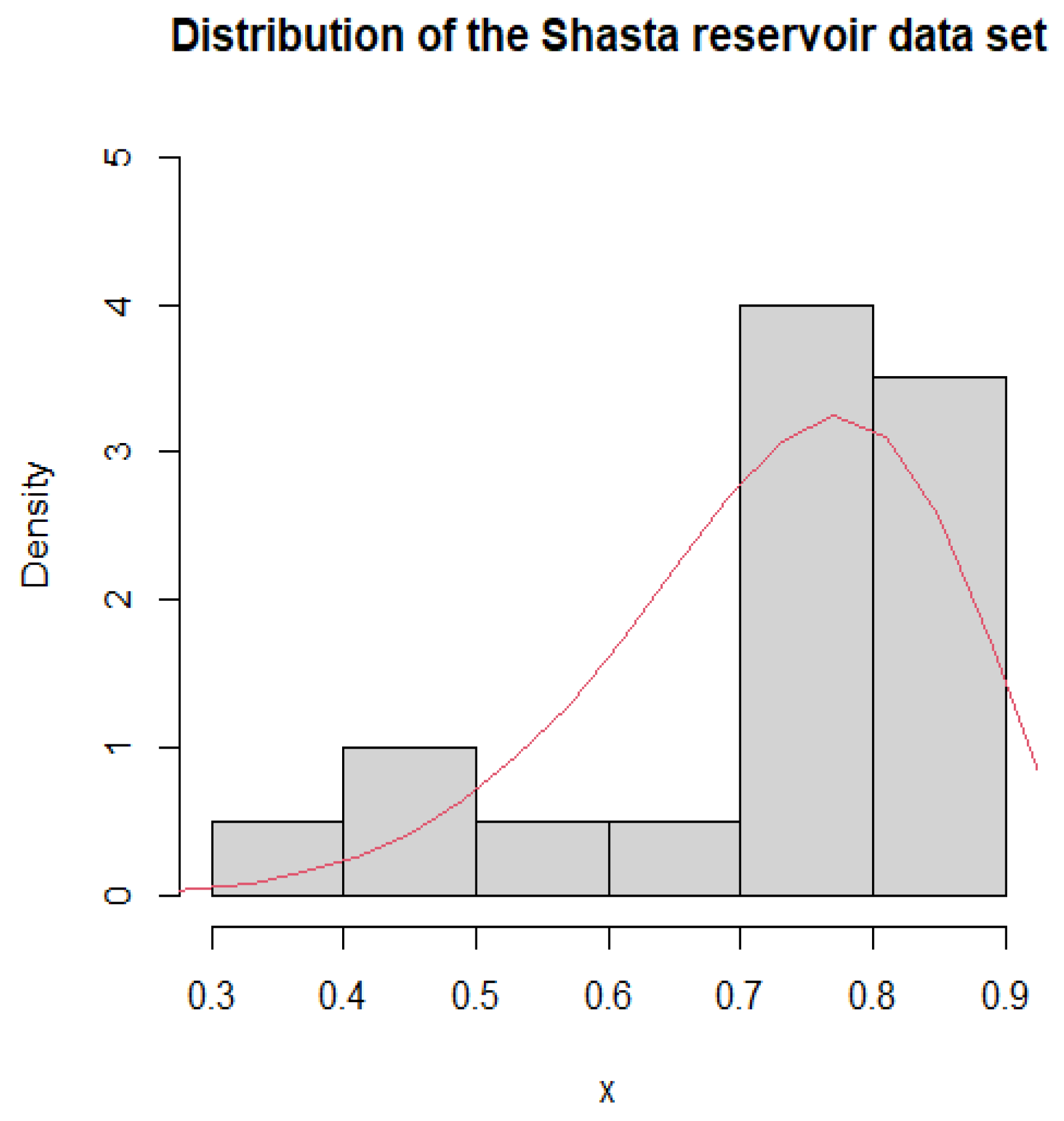
Funding

This research received no external funding.

Data Availability Statement

The source of the datasets are provided in the paper.

Acknowledgments

We would like to thank the reviewers for carefully and thoroughly reading this manuscript and for the thoughtful comments and constructive suggestions, which helped us improve the quality of this manuscript.

Conflicts of Interest

The authors declare no conflict of interest.

Appendix A

Theorem A1 
(Cs o ¨ rgó and Horváth [21]). If 0 < t 1 ( n ) < t 2 ( n ) < 1 and
u ( n ) = 1 t 1 ( n ) t 2 ( n ) t 1 ( n ) ( 1 t 2 ( n ) ) , a s n ;
then we have
lim n P ( A ( log u ( n ) ) sup t 1 ( n ) t t 2 ( n ) M r ( t ) x + D r ( log u ( n ) ) ) = exp ( e x ) ,
for all x.
Corollary A1 
(Cs o ¨ rgó and Horváth [21]). We have for all 0 < λ <
lim n P ( A ( log n ) sup λ / n t < 1 λ / n M r ( t ) x + D r ( log n ) ) = exp ( 2 e x ) , < x < .
Theorem A2 
(Cs o ¨ rgó and Horváth [21]). If H 0 and C 1 C 9 hold; then we have
lim n P A ( log n ) Z n 1 2 t + D d ( log n ) = exp ( 2 e t ) ,
for all t.

References

  1. Page, E.S. Continuous inspection schemes. Biometrika 1954, 41, 100–115. [Google Scholar] [CrossRef]
  2. Page, E.S. A test for a change in a parameter occurring at an unknown point. Biometrika 1955, 42, 523–527. [Google Scholar] [CrossRef]
  3. Sen, A.; Srivastava, M.S. On tests for detecting change in mean. Ann. Stat. 1975, 3, 98–108. [Google Scholar] [CrossRef]
  4. Cai, X.; Said, K.K.; Ning, W. Change-point analysis with bathtub shape for the exponential distribution. J. Appl. Stat. 2016, 43, 2740–2750. [Google Scholar] [CrossRef]
  5. Chen, Y.J.; Ning, W. Information approach for a lifetime change-point model based on the exponential-logarithmic distribution. Commun. Stat.-Simul. Comput. 2019, 48, 1996–2003. [Google Scholar] [CrossRef]
  6. Said, K.K.; Ning, W.; Tian, Y. Modified information criterion for testing changes in skew normal model. Braz. J. Probab. Stat. 2019, 33, 280–300. [Google Scholar] [CrossRef] [Green Version]
  7. Wang, T.; Tian, W.; Ning, W. Likelihood ratio test change-point detection in the skew slash distribution. Commun. Stat.-Simul. Comput. 2020, 1–13. [Google Scholar] [CrossRef]
  8. Tian, W.; Yang, Y. Change point analysis for weighted exponential distribution. Commun. Stat.-Simul. Comput. 2021, 1–13. [Google Scholar] [CrossRef]
  9. Kumaraswamy, P. A generalized probability density function for double-bounded random processes. J. Hydrol. 1980, 46, 79–88. [Google Scholar] [CrossRef]
  10. Jones, M.C. Kumaraswamy’s distribution: A beta-type distribution with some tractability advantages. Stat. Methodol. 2009, 6, 70–81. [Google Scholar] [CrossRef]
  11. Fletcher, S.G.; Ponnambalam, K. Estimation of reservoir yield and storage distribution using moments analysis. J. Hydrol. 1996, 182, 259–275. [Google Scholar] [CrossRef]
  12. Nadarajah, S. On the distribution of kumaraswamy. J. Hydrol. 2008, 348, 568–569. [Google Scholar] [CrossRef]
  13. Nadar, M.; Papadopoulos, A.; Kızılaslan, F. Statistical analysis for Kumaraswamy’s distribution based on record data. Stat. Pap. 2013, 54, 355–369. [Google Scholar] [CrossRef]
  14. Saulo, H.; Leão, J.; Bourguignon, M. The kumaraswamy birnbaum-saunders distribution. J. Stat. Theory Pract. 2012, 6, 745–759. [Google Scholar] [CrossRef]
  15. Lemonte, A.J.; Barreto-Souza, W.; Cordeiro, G.M. The exponentiated Kumaraswamy distribution and its log-transform. Braz. J. Probab. Stat. 2013, 27, 31–53. [Google Scholar] [CrossRef]
  16. Mameli, V. The Kumaraswamy skew-normal distribution. Stat. Probab. Lett. 2015, 104, 75–81. [Google Scholar] [CrossRef] [Green Version]
  17. Iqbal, Z.; Tahir, M.M.; Riaz, N.; Ali, S.A.; Ahmad, M. Generalized inverted Kumaraswamy distribution: Properties and application. Open J. Stat. 2017, 7, 645. [Google Scholar] [CrossRef] [Green Version]
  18. Said, K.K.; Ning, W.; Tian, Y. Likelihood procedure for testing changes in skew normal model with applications to stock returns. Commun. Stat.-Simul. Comput. 2017, 46, 6790–6802. [Google Scholar] [CrossRef]
  19. Zou, C.; Liu, Y.; Qin, P.; Wang, Z. Empirical likelihood ratio test for the change-point problem. Stat. Probab. Lett. 2007, 77, 374–382. [Google Scholar] [CrossRef]
  20. Liu, Z.; Qian, L. Changepoint estimation in a segmented linear regression via empirical likelihood. Commun. Stat.-Simul. Comput. 2009, 39, 85–100. [Google Scholar] [CrossRef]
  21. Csörgó, M.; Horváth, L. Limit Theorems in Change-Point Analysis; John Wiley and Sons Inc.: Hoboken, NJ, USA, 1997; Volume 18. [Google Scholar]
  22. Schwarz, G. Estimating the dimension of a model. Ann. Stat. 1978, 6, 461–464. [Google Scholar] [CrossRef]
  23. Chen, J.; Gupta, A.K.; Pan, J. Information criterion and change point problem for regular models. Sankhya Indian J. Stat. 2006, 68, 252–282. [Google Scholar]
  24. Sultana, F.; Tripathi, Y.M.; Wu, S.J.; Sen, T. Inference for kumaraswamy distribution based on type I progressive hybrid censoring. Ann. Data Sci. 2022, 9, 1283–1307. [Google Scholar] [CrossRef]
  25. Yates, D.; Galbraith, H.; Purkey, D.; Huber-Lee, A.; Sieber, J.; West, J.; Herrod-Julius, S.; Joyce, B. Climate warming, water storage, and Chinook salmon in California’s Sacramento Valley. Clim. Chang. 2008, 91, 335–350. [Google Scholar] [CrossRef]
  26. Khan, M.S.; King, R.; Hudson, I.L. Transmuted kumaraswamy distribution. Stat. Transit. New Ser. 2016, 17, 183–210. [Google Scholar] [CrossRef] [Green Version]
  27. Mazucheli, J.; Menezes, A.F.B.; Ghitany, M.E. The unit-Weibull distribution and associated inference. J. Appl. Probab. Stat. 2018, 13, 1–22. [Google Scholar]
  28. Bantan, R.A.; Chesneau, C.; Jamal, F.; Elgarhy, M.; Almutiry, W.; Alahmadi, A.A. Study of a Modified Kumaraswamy Distribution. Mathematics 2021, 9, 2836. [Google Scholar] [CrossRef]
  29. Roland, M.A.; Underwood, S.M.; Thomas, C.M.; Miller, J.F.; Pratt, B.A.; Hogan, L.G.; Wnek, P.A. Flood-inundation maps for the Susquehanna River near Harrisburg, Pennsylvania, 2013. In Scientific Investigations Report 2014–5046; US Geological Survey: Reston, VA, USA, 2014; Volume 28. [Google Scholar]
  30. Elgarhy, M. Exponentiated generalized Kumaraswamy distribution with applications. Ann. Data Sci. 2018, 5, 273–292. [Google Scholar] [CrossRef]
Figure 1. Histogram and PDF fitting of Shasta reservoir dataset.
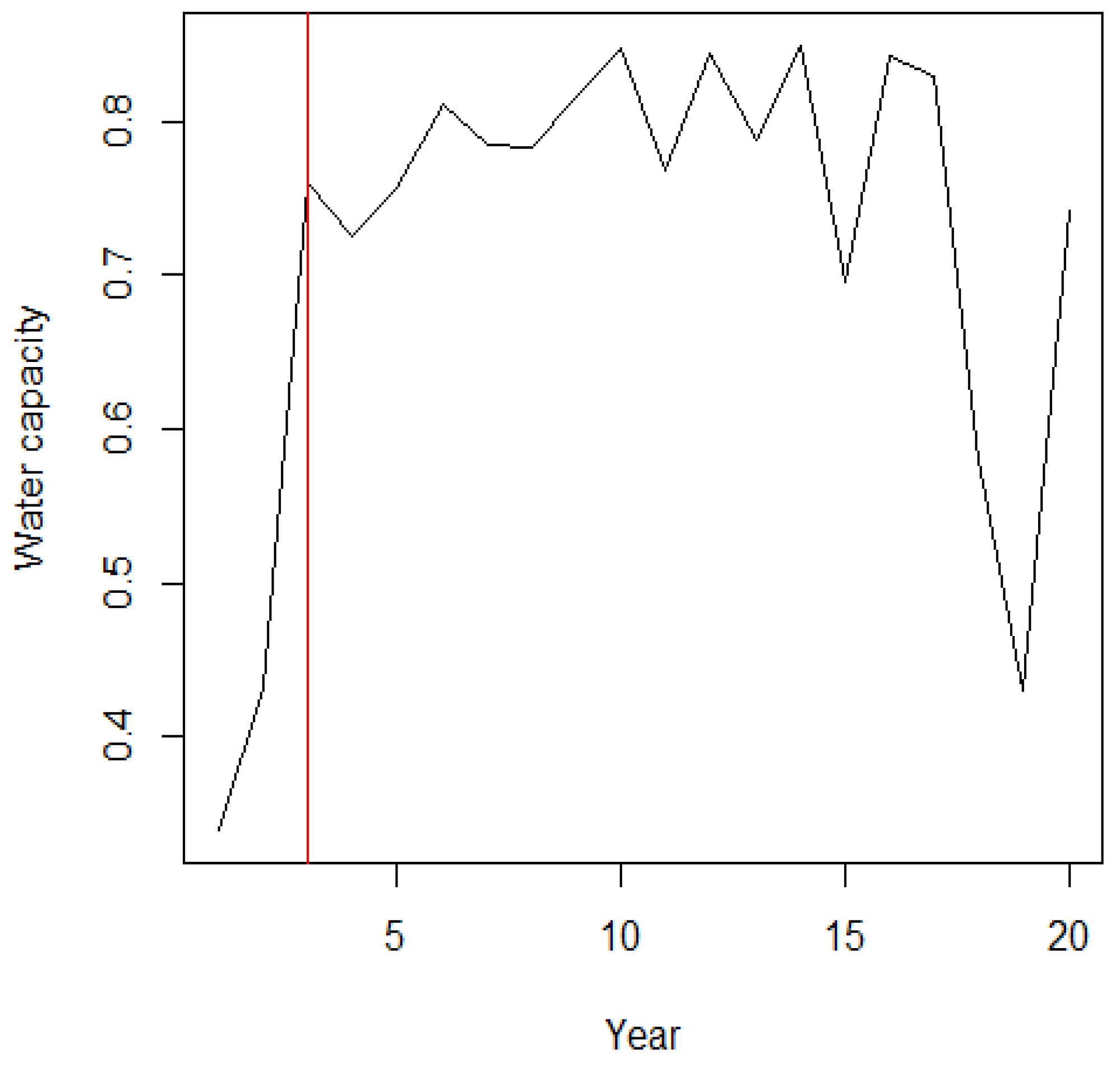
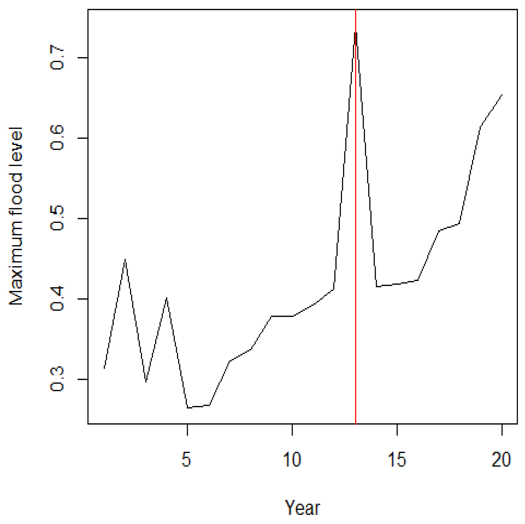
Mathematics 11 00553 g001
Figure 2. The Shasta reservoir dataset and position of change point.
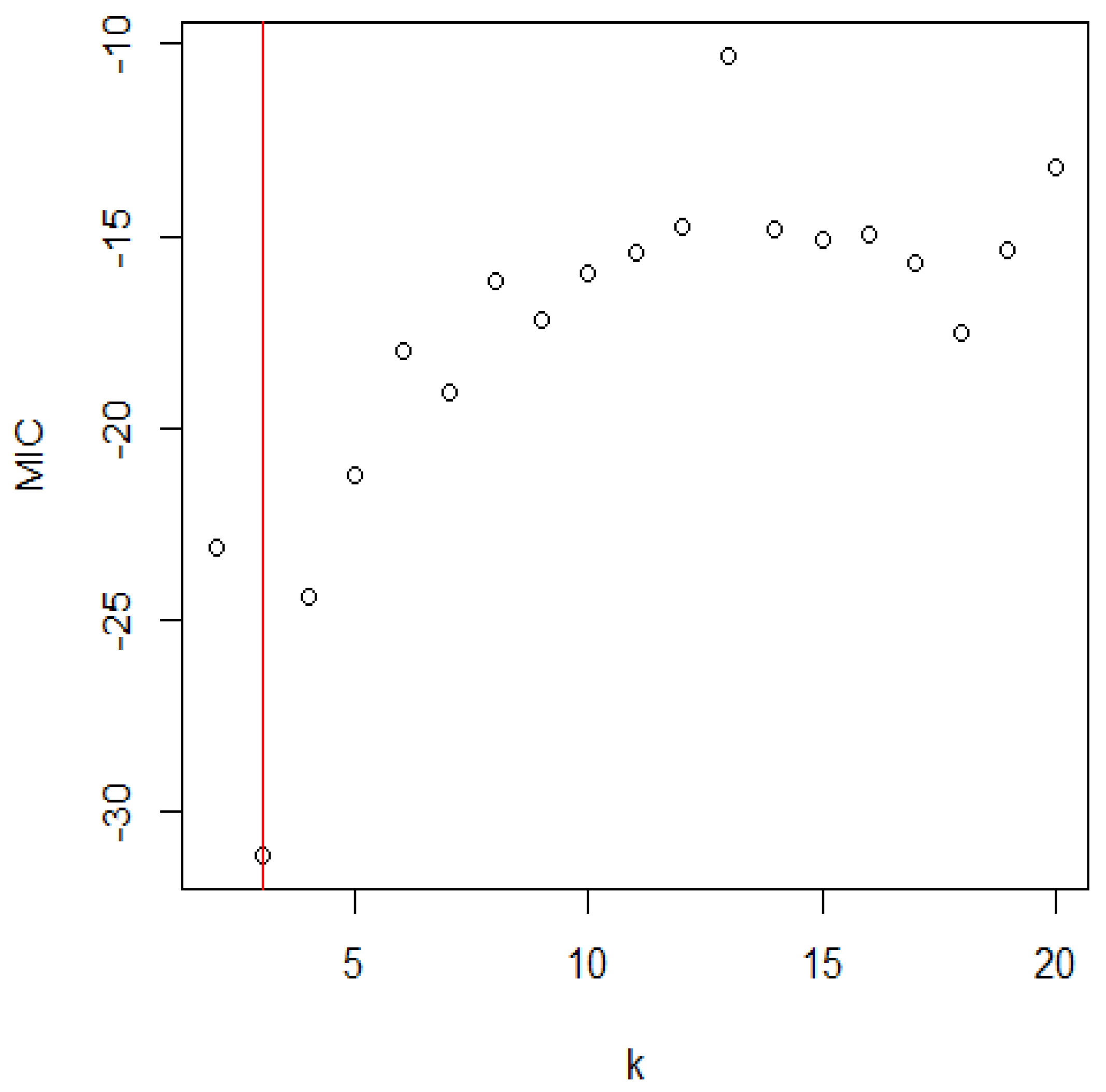
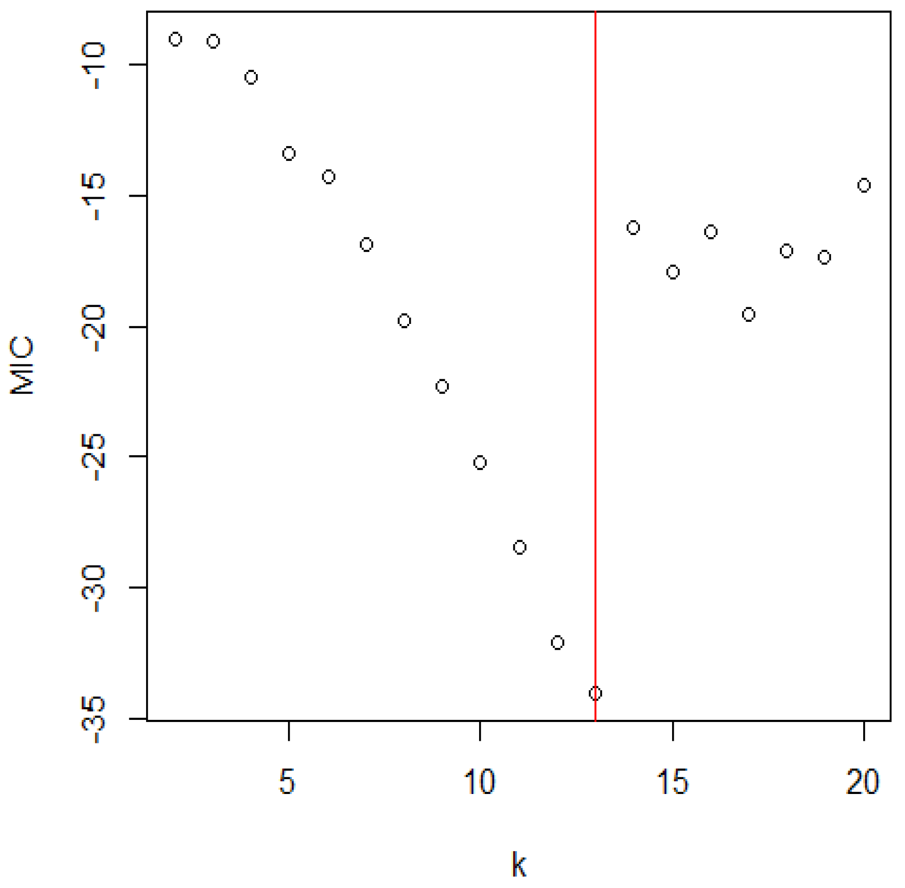
Mathematics 11 00553 g002
Figure 3. The distribution of MIC for the Shasta reservoir.
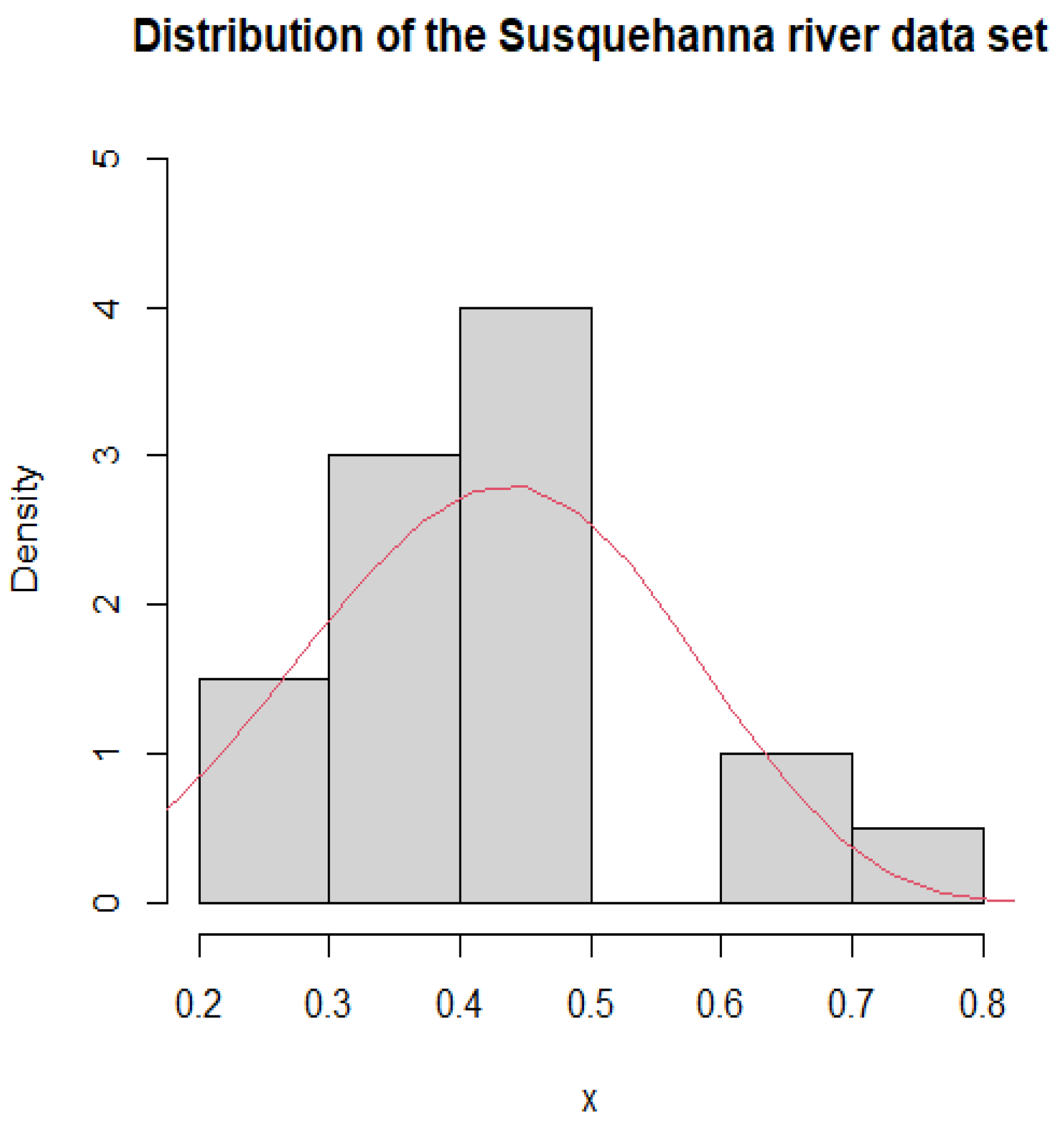
Mathematics 11 00553 g003
Figure 4. Histogram and PDF fitting of Susquehanna river dataset.
Mathematics 11 00553 g004
Figure 5. The Susquehanna river dataset and position of change point.
Mathematics 11 00553 g005
Figure 6. The distribution of MIC for the Susquehanna river.
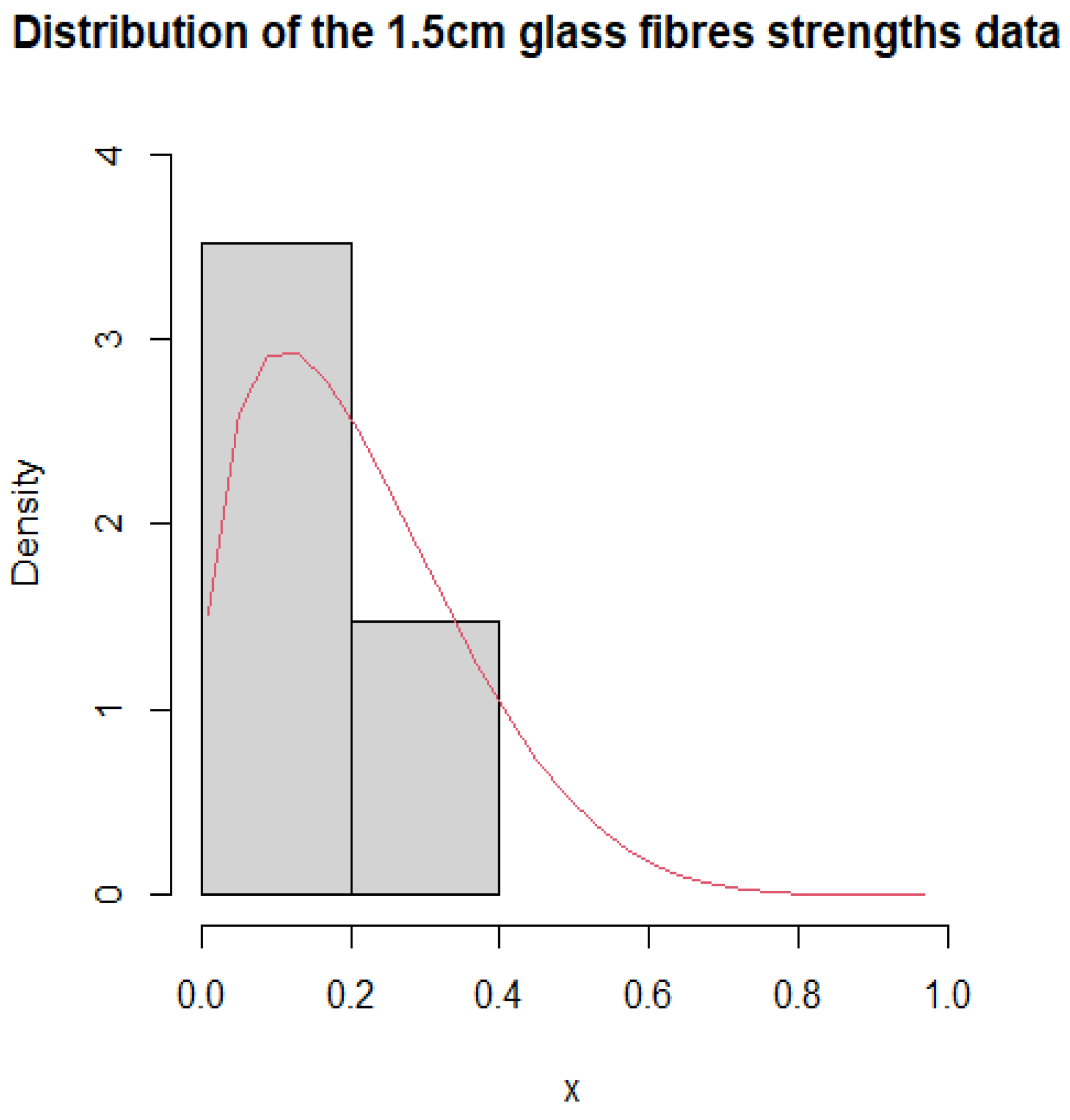
Mathematics 11 00553 g006
Figure 7. Histogram and PDF fitting of 1.5 cm glass fibre strengths dataset.
Mathematics 11 00553 g007
Figure 8. The strengths of 1.5cm glass fibres dataset and position of change point.
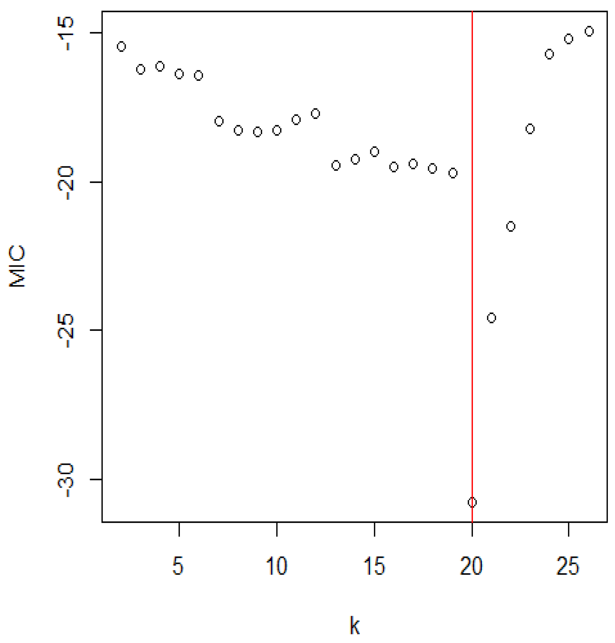
Mathematics 11 00553 g008
Figure 9. The distribution of the MIC for the strengths of 1.5 cm glass fibres.
Mathematics 11 00553 g009
Table 1. Approximate critical values of LRT with different values of α and n.
n α = 0.01 α = 0.05 α = 0.1 n α = 0.01 α = 0.05 α = 0.1
1527.947812.67448.85119021.366813.686210.8365
2021.614712.63869.440110021.374513.788910.9661
3521.480712.88479.784211021.384512.638611.0768
4021.420713.076810.044012021.395713.955111.1734
5021.372513.360210.418214021.419114.085611.3344
6021.388913.231510.249616021.405014.010811.2422
7021.367913.417010.492018021.423814.108611.3626
8021.363313.564610.681920021.442514.192211.4649
Table 2. Approximate critical values of SIC with different values of α and n.
n α = 0.01 α = 0.05 α = 0.1 n α = 0.01 α = 0.05 α = 0.1
1521.198210.61716.79327016.80388.08194.8147
2020.194910.14446.47668016.49027.85924.6200
2519.50079.77906.20919016.21787.66234.4463
3018.97269.48045.979310015.97727.48574.2894
3518.54769.22755.778215015.07406.80203.6737
4018.19279.00805.599720014.45076.31333.2268
5017.62228.64005.293225013.97515.93212.8751
6017.17338.33815.036230013.59075.61932.5847
Table 3. Approximate critical values for MIC under different parameters.
n Kw ( · ) α = 0.01 α = 0.05 α = 0.1 Kw ( · ) α = 0.01 α = 0.05 α = 0.1
15 ( 4 , 0.5 ) 16.021412.14409.9910 ( 0.5 , 3.5 ) 12.78058.41316.6169
20 ( 4 , 0.5 ) 13.53489.41297.7097 ( 0.5 , 3.5 ) 9.17974.83043.0177
30 ( 4 , 0.5 ) 12.52919.38807.2124 ( 0.5 , 3.5 ) 14.61269.00676.5348
40 ( 4 , 0.5 ) 12.46419.42817.4635 ( 0.5 , 3.5 ) 13.33778.60045.0923
50 ( 4 , 0.5 ) 11.62237.68736.0628 ( 0.5 , 3.5 ) 12.02177.27455.1606
55 ( 4 , 0.5 ) 15.256012.156010.1627 ( 0.5 , 3.5 ) 16.448113.065211.7789
60 ( 4 , 0.5 ) 19.790813.645411.8123 ( 0.5 , 3.5 ) 16.110912.278310.4150
80 ( 4 , 0.5 ) 17.772013.565011.3690 ( 0.5 , 3.5 ) 16.770412.321610.3872
100 ( 4 , 0.5 ) 17.469712.903510.9909 ( 0.5 , 3.5 ) 10.04376.77114.1757
150 ( 4 , 0.5 ) 18.080113.001311.0911 ( 0.5 , 3.5 ) 15.043711.771110.1757
200 ( 4 , 0.5 ) 16.245212.557310.6762 ( 0.5 , 3.5 ) 15.584811.949910.0195
Table 4. Approximate critical values for MIC under parameters.
n Kw ( · ) α = 0.01 α = 0.05 α = 0.1
15 ( 5 , 2 ) 19.460412.966910.3656
20 ( 5 , 2 ) 18.407013.095810.5379
30 ( 5 , 2 ) 21.836316.095814.8520
40 ( 5 , 2 ) 17.591913.954911.5930
50 ( 5 , 2 ) 17.200310.82308.3099
55 ( 5 , 2 ) 18.294613.923211.8138
60 ( 5 , 2 ) 17.961013.112911.1608
80 ( 5 , 2 ) 16.435612.117710.8341
100 ( 5 , 2 ) 11.37327.00836.4604
150 ( 5 , 2 ) 15.226411.80869.2993
200 ( 5 , 2 ) 15.629412.164910.5434
Table 5. Powers of the LRT, SIC, and MIC procedures at ( γ 1 , β 1 ) = ( 4 , 0.5 ) , n = 20 .
( γ n , β n )
α kModel ( γ 1 , β 1 ) (4, 2.5)(0.2, 0.5)(2, 2)(4, 0.5)
0.015LRT(4, 0.5)0.1160.0370.1460.000
SIC(4, 0.5)0.0480.0150.0750.000
MIC(4, 0.5)0.4830.5940.6100.016
10LRT(4, 0.5)0.1070.2480.1870.001
SIC(4, 0.5)0.0240.0760.0860.000
MIC(4, 0.5)0.5670.8090.7070.018
15LRT(4, 0.5)0.0360.2250.0790.004
SIC(4, 0.5)0.0080.1590.0180.000
MIC(4, 0.5)0.5920.8040.5830.015
0.055LRT(4, 0.5)0.5200.4710.6410.027
SIC(4, 0.5)0.3420.2350.4340.012
MIC(4, 0.5)0.7340.7730.8570.033
10LRT(4, 0.5)0.6010.8460.7800.029
SIC(4, 0.5)0.3370.6150.5510.026
MIC(4, 0.5)0.8380.9680.9300.037
15LRT(4, 0.5)0.3260.8150.5420.025
SIC(4, 0.5)0.1480.6650.2750.013
MIC(4, 0.5)0.6560.9320.8040.029
0.15LRT(4, 0.5)0.7260.7820.8310.049
SIC(4, 0.5)0.5580.5100.6730.030
MIC(4, 0.5)0.8530.9280.9120.065
10LRT(4, 0.5)0.8130.9620.9230.051
SIC(4, 0.5)0.5830.8400.7940.037
MIC(4, 0.5)0.9120.9880.9750.065
15LRT(4, 0.5)0.6100.8930.7780.030
SIC(4, 0.5)0.3540.8350.5490.017
MIC(4, 0.5)0.7820.9700.9080.037
Table 6. Powers of the LRT, SIC, and MIC procedures at ( γ 1 , β 1 ) = ( 4 , 0.5 ) , n = 50 .
( γ n , β n )
α kModel ( γ 1 , β 1 ) (4, 2.5)(0.2, 0.5)(2, 2)(4, 0.5)
0.0115LRT(4, 0.5)0.7950.8690.9300.000
SIC(4, 0.5)0.6170.6720.8370.000
MIC(4, 0.5)0.9790.9980.9980.002
25LRT(4, 0.5)0.8280.9950.9550.001
SIC(4, 0.5)0.6390.9600.9040.000
MIC(4, 0.5)0.9961.0001.0000.006
35LRT(4, 0.5)0.5300.9880.9770.002
SIC(4, 0.5)0.3000.9760.7180.000
MIC(4, 0.5)0.9640.9990.9940.002
0.0515LRT(4, 0.5)0.9630.9960.9980.012
SIC(4, 0.5)0.9300.9830.9830.006
MIC(4, 0.5)0.9961.0001.0000.014
25LRT(4, 0.5)0.9861.0000.9990.022
SIC(4, 0.5)0.9550.9980.9950.004
MIC(4, 0.5)1.0001.0001.0000.034
35LRT(4, 0.5)0.9360.9990.9960.010
SIC(4, 0.5)0.8100.9970.9780.009
MIC(4, 0.5)0.9981.0001.0000.011
0.115LRT(4, 0.5)0.9911.0000.9990.026
SIC(4, 0.5)0.9740.9960.9930.024
MIC(4, 0.5)0.9991.0001.0000.032
25LRT(4, 0.5)0.9971.0001.0000.029
SIC(4, 0.5)0.9921.0000.9990.029
MIC(4, 0.5)1.0001.0001.0000.034
35LRT(4, 0.5)0.9890.9990.9990.017
SIC(4, 0.5)0.9310.9980.9960.011
MIC(4, 0.5)1.0001.0001.0000.028
Table 7. Powers of the LRT, SIC, and MIC procedures at ( γ 1 , β 1 ) = ( 4 , 0.5 ) , n = 100 .
( γ n , β n )
α kModel ( γ 1 , β 1 ) (4, 2.5)(0.2, 0.5)(2, 2)(4, 0.5)
0.0125LRT(4, 0.5)0.9951.0000.9980.002
SIC(4, 0.5)0.9891.0000.9970.001
MIC(4, 0.5)0.9991.0001.0000.008
50LRT(4, 0.5)1.0001.0001.0000.000
SIC(4, 0.5)0.9981.0001.0000.000
MIC(4, 0.5)1.0001.0001.0000.005
75LRT(4, 0.5)0.9721.0001.0000.002
SIC(4, 0.5)0.9131.0000.9960.000
MIC(4, 0.5)0.9911.0001.0000.006
0.0525LRT(4, 0.5)1.0001.0001.0000.033
SIC(4, 0.5)0.9991.0001.0000.006
MIC(4, 0.5)1.0001.0001.0000.046
50LRT(4, 0.5)1.0001.0001.0000.023
SIC(4, 0.5)1.0001.0001.0000.012
MIC(4, 0.5)1.0001.0001.0000.051
75LRT(4, 0.5)0.9991.0001.0000.034
SIC(4, 0.5)0.9991.0001.0000.010
MIC(4, 0.5)0.9991.0001.0000.042
0.125LRT(4, 0.5)1.0001.0001.0000.075
SIC(4, 0.5)1.0001.0001.0000.033
MIC(4, 0.5)1.0001.0001.0000.093
50LRT(4, 0.5)1.0001.0001.0000.072
SIC(4, 0.5)1.0001.0001.0000.040
MIC(4, 0.5)1.0001.0001.0000.099
75LRT(4, 0.5)1.0001.0001.0000.094
SIC(4, 0.5)1.0001.0001.0000.039
MIC(4, 0.5)1.0001.0001.0000.096
Table 8. Powers of the LRT, SIC, and MIC procedures at ( γ 1 , β 1 ) = ( 0.5 , 3.5 ) , n = 20 .
( γ n , β n )
α kModel ( γ 1 , β 1 ) (0.5, 1.5)(1.2, 3.5)(0.8, 2.5)(0.5, 3.5)
0.015LRT(0.5, 3.5)0.1650.3880.2080.001
SIC(0.5, 3.5)0.1050.2710.1620.000
MIC(0.5, 3.5)0.4230.6800.4950.003
10LRT(0.5, 3.5)0.2460.4930.3270.001
SIC(0.5, 3.5)0.1620.3200.2180.000
MIC(0.5, 3.5)0.5140.8120.5700.006
15LRT(0.5, 3.5)0.2010.2680.2540.001
SIC(0.5, 3.5)0.1110.1510.1590.000
MIC(0.5, 3.5)0.4500.6770.4770.002
0.055LRT(0.5, 3.5)0.4460.6940.5180.028
SIC(0.5, 3.5)0.3340.5860.4110.004
MIC(0.5, 3.5)0.8790.9530.8920.036
10LRT(0.5, 3.5)0.5430.7940.6160.045
SIC(0.5, 3.5)0.3940.7360.4690.017
MIC(0.5, 3.5)0.9030.9870.9230.059
15LRT(0.5, 3.5)0.4760.5990,5170.024
SIC(0.5, 3.5)0.3000.5420.3770.006
MIC(0.5, 3.5)0.8660.9590.8980.039
0.15LRT(0.5, 3.5)0.7630.8750.8330.043
SIC(0.5, 3.5)0.5810.7610.6430.031
MIC(0.5, 3.5)0.9890.9990.9970.056
10LRT(0.5, 3.5)0.8230.9280.8890.054
SIC(0.5, 3.5)0.6280.8750.7130.048
MIC(0.5, 3.5)0.9991.0000.9980.078
15LRT(0.5, 3.5)0.7810.8850.8140.049
SIC(0.5, 3.5)0.5260.7470.6380.034
MIC(0.5, 3.5)0.9920.9980.9980.061
Table 9. Powers of the LRT, SIC, and MIC procedures at ( γ 1 , β 1 ) = ( 0.5 , 3.5 ) , n = 50 .
( γ n , β n )
α kModel ( γ 1 , β 1 ) (0.5, 1.5)(1.2, 3.5)(0.8, 2.5)(0.5, 3.5)
0.0115LRT(0.5, 3.5)0.5430.8890.7350.001
SIC(0.5, 3.5)0.3260.7500.5510.000
MIC(0.5, 3.5)0.7900.9870.8200.010
25LRT(0.5, 3.5)0.6390.9320.8250.004
SIC(0.5, 3.5)0.4260.8410.6240.001
MIC(0.5, 3.5)0.8970.9950.9010.015
35LRT(0.5, 3.5)0.5880.8050.7440.000
SIC(0.5, 3.5)0.3650.6480.5470.000
MIC(0.5, 3.5)0.8320.9810.8270.007
0.0515LRT(0.5, 3.5)0.7240.9750.8440.029
SIC(0.5, 3.5)0.6080.9290.8100.010
MIC(0.5, 3.5)0.9290.9990.9650.033
25LRT(0.5, 3.5)0.8030.9890.9060.033
SIC(0.5, 3.5)0.7420.9560.8580.010
MIC(0.5, 3.5)0.9541.0000.9880.048
35LRT(0.5, 3.5)0.7320.9660,8500.034
SIC(0.5, 3.5)0.6350.8860.7890.012
MIC(0.5, 3.5)0.9260.9990.9710.048
0.115LRT(0.5, 3.5)0.9220.9940.9680.070
SIC(0.5, 3.5)0.7200.9690.8170.031
MIC(0.5, 3.5)0.9921.0000.9970.085
25LRT(0.5, 3.5)0.9501.0000.9800.079
SIC(0.5, 3.5)0.8230.9860.9160.033
MIC(0.5, 3.5)0.9991.0001.0000.095
35LRT(0.5, 3.5)0.9080.9960.9500.077
SIC(0.5, 3.5)0.7490.9520.8680.035
MIC(0.5, 3.5)0.9881.0000.9990.090
Table 10. Powers of the LRT, SIC, and MIC procedures at ( γ 1 , β 1 ) = ( 0.5 , 3.5 ) , n = 100 .
( γ n , β n )
α kModel ( γ 1 , β 1 ) (0.5, 1.5)(1.2, 3.5)(0.8, 2.5)(0.5, 3.5)
0.0125LRT(0.5, 3.5)0.7730.9740.8210.002
SIC(0.5, 3.5)0.6180.9320.6930.001
MIC(0.5, 3.5)0.8901.0000.9450.011
50LRT(0.5, 3.5)0.8400.9960.8540.007
SIC(0.5, 3.5)0.7590.9840.7630.001
MIC(0.5, 3.5)0.9811.0000.9930.019
75LRT(0.5, 3.5)0.8350.9480.8390.002
SIC(0.5, 3.5)0.6250.9080.6380.000
MIC(0.5, 3.5)0.9191.0000.9490.007
0.0525LRT(0.5, 3.5)0.8090.9970.8800.032
SIC(0.5, 3.5)0.6730.9930.8570.007
MIC(0.5, 3.5)0.9391.0000.9940.060
50LRT(0.5, 3.5)0.8951.0000.9570.038
SIC(0.5, 3.5)0.7801.0000.9110.012
MIC(0.5, 3.5)0.9921.0000.9980.074
75LRT(0.5, 3.5)0.8190.9960,8700.025
SIC(0.5, 3.5)0.6740.9960.8130.007
MIC(0.5, 3.5)0.9551.0000.9920.039
0.125LRT(0.5, 3.5)0.9431.0000.9890.076
SIC(0.5, 3.5)0.8330.9960.9000.037
MIC(0.5, 3.5)0.9971.0001.0000.087
50LRT(0.5, 3.5)0.9871.0000.9950.080
SIC(0.5, 3.5)0.8901.0000.9630.029
MIC(0.5, 3.5)0.9991.0001.0000.090
75LRT(0.5, 3.5)0.9451.0000.9920.064
SIC(0.5, 3.5)0.8471.0000.8950.034
MIC(0.5, 3.5)0.9921.0001.0000.082
Table 11. Powers of the LRT, SIC, and MIC procedures at ( γ 1 , β 1 ) = ( 5 , 2 ) , n = 20 .
( γ n , β n )
α kModel ( γ 1 , β 1 ) (5, 3.5)(0.5, 2)(1.5, 4.5)(5, 2)
0.015LRT(5, 2)0.2740.2630.2950.000
SIC(5, 2)0.0990.1140.1180.000
MIC(5, 2)0.4830.6000.5130.007
10LRT(5, 2)0.3810.4940.3330.002
SIC(5, 2)0.1440.2180.1190.000
MIC(5, 2)0.6860.7490.8080.007
15LRT(5, 2)0.1860.3580.1520.001
SIC(5, 2)0.0690.1440.0360.000
MIC(5, 2)0.4450.6170.6110.005
0.055LRT(5, 2)0.6700.7960.8480.013
SIC(5, 2)0.5140.5990.6350.004
MIC(5, 2)0.7490.9260.8700.050
10LRT(5, 2)0.8280.8870.9630.038
SIC(5, 2)0.6480.6840.8640.006
MIC(5, 2)0.8850.9740.9680.063
15LRT(5, 2)0.6590.6940,8180.043
SIC(5, 2)0.3190.3580.7310.005
MIC(5, 2)0.7500.9540.8040.059
0.15LRT(5, 2)0.7430.9220.8840.053
SIC(5, 2)0.6290.7840.8610.049
MIC(5, 2)0.8230.9830.9570.074
10LRT(5, 2)0.7820.9750.8940.062
SIC(5, 2)0.6350.8880.8810.051
MIC(5, 2)0.8570.9980.9960.080
15LRT(5, 2)0.6230.8710.8830.049
SIC(5, 2)0.5690.6580.8200.043
MIC(5, 2)0.8350.9960.9680.080
Table 12. Powers of the LRT, SIC, and MIC procedures at ( γ 1 , β 1 ) = ( 5 , 2 ) , n = 50 .
( γ n , β n )
α kModel ( γ 1 , β 1 ) (5, 3.5)(0.5, 2)(1.5, 4.5)(5, 2)
0.0115LRT(5, 2)0.5120.8860.9990.001
SIC(5, 2)0.4030.7190.9980.001
MIC(5, 2)0.6001.0001.0000.004
25LRT(5, 2)0.5190.9541.0000.002
SIC(5, 2)0.4150.7611.0000.001
MIC(5, 2)0.6491.0001.0000.013
35LRT(5, 2)0.5070.9321.0000.000
SIC(5, 2)0.4040.7540.9980.000
MIC(5, 2)0.6121.0001.0000.005
0.0515LRT(5, 2)0.8320.9971.0000.028
SIC(5, 2)0.6680.8421.0000.008
MIC(5, 2)0.8341.0001.0000.035
25LRT(5, 2)0.8940.9991.0000.036
SIC(5, 2)0.6700.8531.0000.011
MIC(5, 2)0.8661.0001.0000.048
35LRT(5, 2)0.8140.8781.0000.017
SIC(5, 2)0.6550.7961.0000.008
MIC(5, 2)0.8481.0001.0000.027
0.115LRT(5, 2)0.9091.0001.0000.064
SIC(5, 2)0.7770.9981.0000.028
MIC(5, 2)0.9481.0001.0000.078
25LRT(5, 2)0.9231.0001.0000.069
SIC(5, 2)0.7960.9991.0000.038
MIC(5, 2)0.9621.0001.0000.083
35LRT(5, 2)0.8811.0001.0000.050
SIC(5, 2)0.7370.9791.0000.031
MIC(5, 2)0.9581.0001.0000.081
Table 13. Powers of the LRT, SIC, and MIC procedures at ( γ 1 , β 1 ) = ( 5 , 2 ) , n = 100 .
( γ n , β n )
α kModel ( γ 1 , β 1 ) (5, 3.5)(0.5, 2)(1.5, 4.5)(5, 2)
0.0125LRT(5, 2)0.7550.9171.0000.002
SIC(5, 2)0.6280.7671.0000.000
MIC(5, 2)0.7991.0001.0000.009
50LRT(5, 2)0.8690.9931.0000.003
SIC(5, 2)0.7220.8691.0000.001
MIC(5, 2)0.8901.0001.0000.013
75LRT(5, 2)0.8320.9621.0000.002
SIC(5, 2)0.7100.8141.0000.001
MIC(5, 2)0.7651.0001.0000.010
0.0525LRT(5, 2)0.8940.9991.0000.035
SIC(5, 2)0.7750.8601.0000.008
MIC(5, 2)0.9371.0001.0000.061
50LRT(5, 2)0.9450.9491.0000.039
SIC(5, 2)0.8040.9211.0000.009
MIC(5, 2)0.9791.0001.0000.071
75LRT(5, 2)0.8480.9731.0000.025
SIC(5, 2)0.7160.8851.0000.009
MIC(5, 2)0.9401.0001.0000.067
0.125LRT(5, 2)0.9791.0001.0000.065
SIC(5, 2)0.8980.9981.0000.028
MIC(5, 2)0.9891.0001.0000.086
50LRT(5, 2)0.9841.0001.0000.081
SIC(5, 2)0.9181.0001.0000.037
MIC(5, 2)0.9971.0001.0000.091
75LRT(5, 2)0.9431.0001.0000.075
SIC(5, 2)0.8520.9991.0000.030
MIC(5, 2)0.9921.0001.0000.087
Table 14. The MLEs and the goodness-of-fit statistics for the Shasta reservoir dataset.
Modeln γ ^ β ^ K–S (pval)
K w 206.0604.0830.221 (0.245)
Table 15. The MLEs and the goodness-of-fit statistics for Susquehanna river dataset.
Modeln γ ^ β ^ K–S (pval)
K w 203.35311.6580.213 (0.284)
Table 16. The MLEs and the goodness-of-fit statistics for 1.5cm glass fibre strengths dataset.
Modeln γ ^ β ^ K–S (pval)
K w 271.3836.4610.240 (0.074)
Disclaimer/Publisher’s Note: The statements, opinions and data contained in all publications are solely those of the individual author(s) and contributor(s) and not of MDPI and/or the editor(s). MDPI and/or the editor(s) disclaim responsibility for any injury to people or property resulting from any ideas, methods, instructions or products referred to in the content.

