A Neural Network Decomposition Algorithm for Mapping on Crossbar-Based Computing Systems


Abstract
:1. Introduction
2. Problem Formulation
3. Decomposition Algorithms
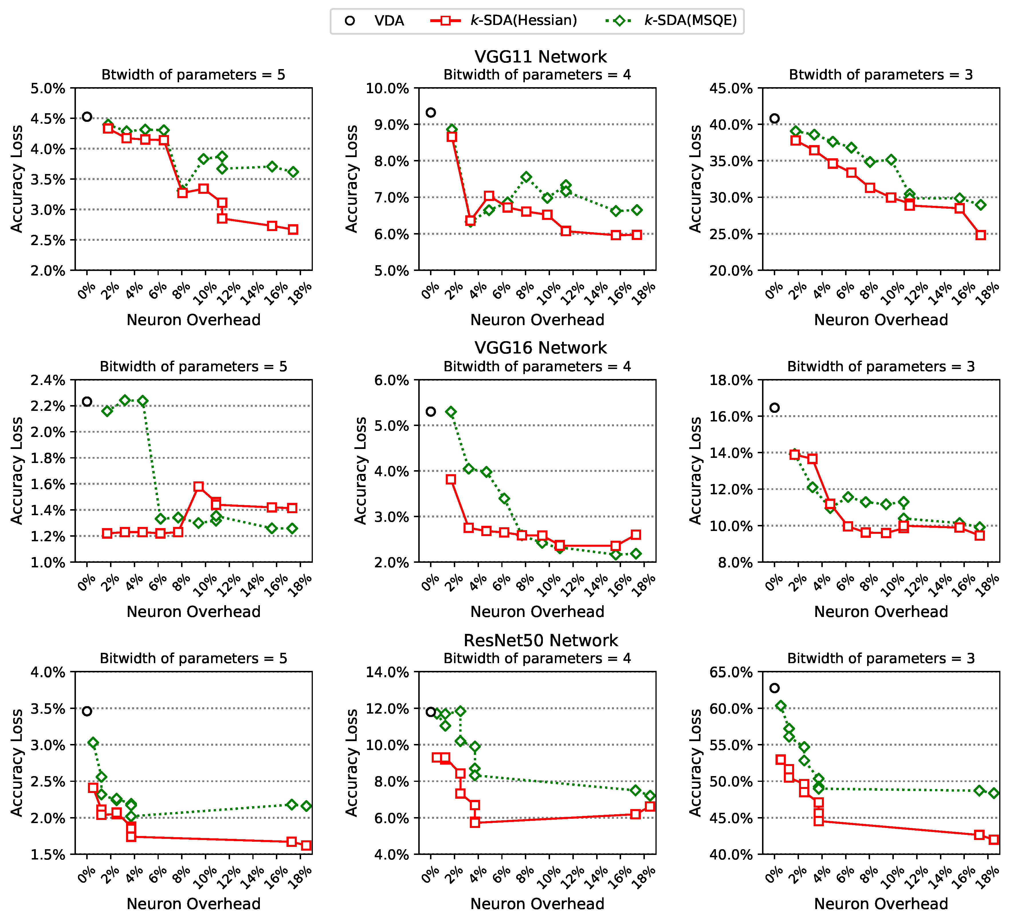
3.1. Vanilla Decomposition Algorithm (VDA)
3.2. k-Spare Decomposition Algorithm (k-SDA)
3.2.1. Global Decomposition
3.2.2. Local Decomposition
4. Local Decomposition Methods
4.1. Candidate Selection
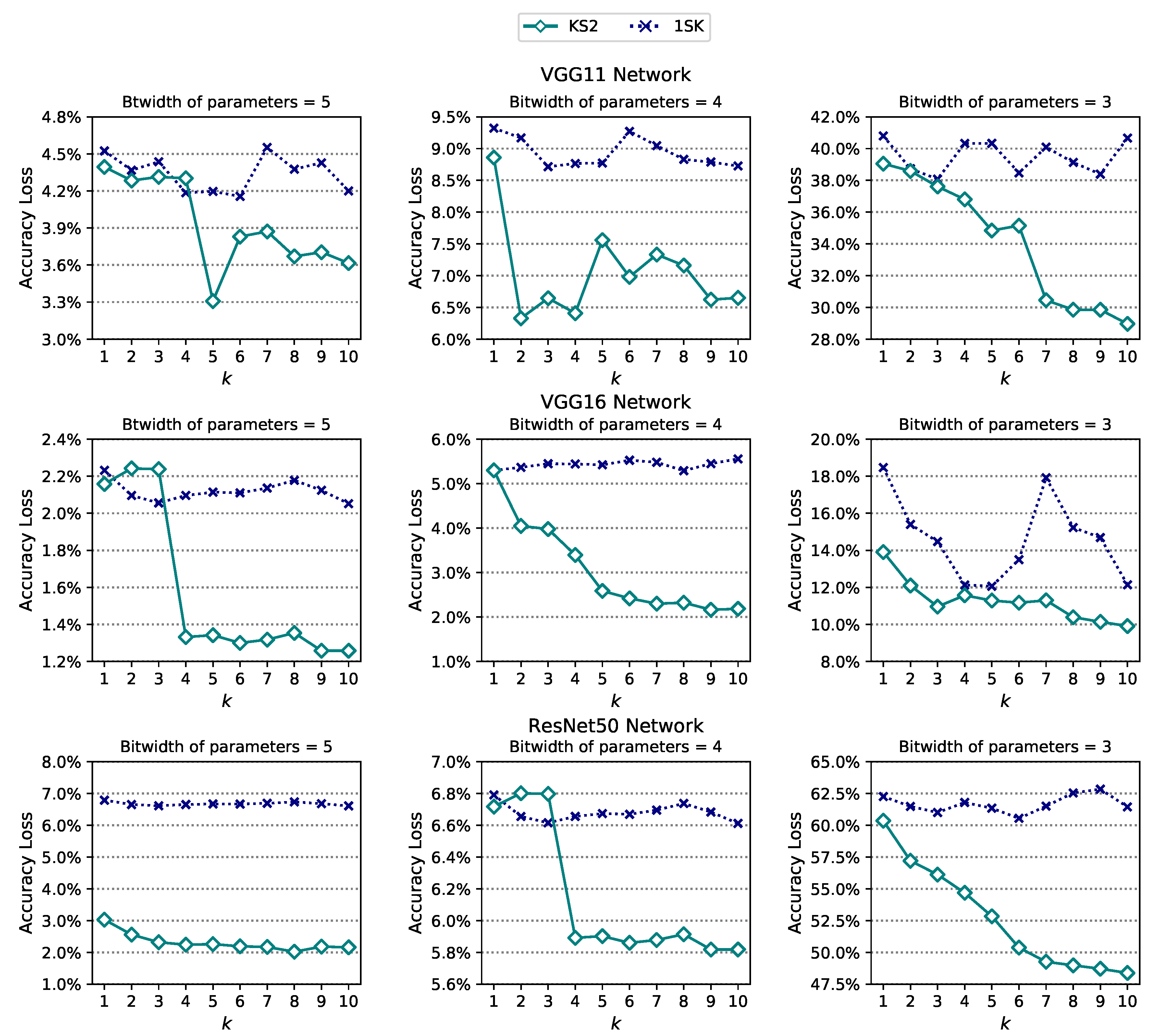
4.2. k Split-in-Two (KS2)
4.3. One Split-in- (1SK)
5. Experimental Results
6. Conclusions
Author Contributions
Funding
Conflicts of Interest
References
- LeCun, Y.; Bengio, Y.; Hinton, G. Deep learning. Nature 2015, 521, 436–444. [Google Scholar] [CrossRef] [PubMed]
- Simonyan, K.; Zisserman, A. Very deep convolutional networks for large-scale image recognition. arXiv 2014, arXiv:1409.1556. [Google Scholar]
- Silver, D.; Huang, A.; Maddison, C.J.; Guez, A.; Sifre, L.; Van Den Driessche, G.; Schrittwieser, J.; Antonoglou, I.; Panneershelvam, V.; Lanctot, M.; et al. Mastering the game of Go with deep neural networks and tree search. Nature 2016, 529, 484–489. [Google Scholar] [CrossRef] [PubMed]
- Han, S.; Dally, B. Efficient Methods and Hardware for Deep Learning; University Lecture; Stanford University: Stanford, CA, USA, 2017. [Google Scholar]
- Mahapatra, N.R.; Venkatrao, B. The processor-memory bottleneck: Problems and solutions. Crossroads 1999, 5, 2. [Google Scholar] [CrossRef]
- Lacey, G.; Taylor, G.W.; Areibi, S. Deep learning on fpgas: Past, present, and future. arXiv 2016, arXiv:1602.04283. [Google Scholar]
- Wang, J.; Lin, J.; Wang, Z. Efficient hardware architectures for deep convolutional neural network. IEEE Trans. Circuits Syst. I Regul. Pap. 2017, 65, 1941–1953. [Google Scholar] [CrossRef]
- Stromatias, E.; Galluppi, F.; Patterson, C.; Furber, S. Power analysis of large-scale, real-time neural networks on SpiNNaker. In Proceedings of the 2013 International Joint Conference on Neural Networks (IJCNN), Dallas, TX, USA, 4–9 August 2013; pp. 1–8. [Google Scholar]
- Mead, C. Neuromorphic electronic systems. Proc. IEEE 1990, 78, 1629–1636. [Google Scholar] [CrossRef] [Green Version]
- Chung, J.; Shin, T.; Kang, Y. Insight: A neuromorphic computing system for evaluation of large neural networks. arXiv 2015, arXiv:1508.01008. [Google Scholar]
- Akopyan, F.; Sawada, J.; Cassidy, A.; Alvarez-Icaza, R.; Arthur, J.; Merolla, P.; Imam, N.; Nakamura, Y.; Datta, P.; Nam, G.J.; et al. Truenorth: Design and tool flow of a 65 mw 1 million neuron programmable neurosynaptic chip. IEEE Trans. Comput. Aided Des. Integr. Circuits Syst. 2015, 34, 1537–1557. [Google Scholar] [CrossRef]
- Kang, Y.; Yang, J.S.; Chung, J. Weight Partitioning for Dynamic Fixed-Point Neuromorphic Computing Systems. IEEE Trans. Comput. Aided Des. Integr. Circuits Syst. 2018, 38, 2167–2171. [Google Scholar] [CrossRef]
- Chi, P.; Li, S.; Xu, C.; Zhang, T.; Zhao, J.; Liu, Y.; Wang, Y.; Xie, Y. Prime: A novel processing-in-memory architecture for neural network computation in reram-based main memory. ACM SIGARCH Comput. Archit. News 2016, 44, 27–39. [Google Scholar] [CrossRef]
- Shafiee, A.; Nag, A.; Muralimanohar, N.; Balasubramonian, R.; Strachan, J.P.; Hu, M.; Williams, R.S.; Srikumar, V. ISAAC: A convolutional neural network accelerator with in-situ analog arithmetic in crossbars. ACM SIGARCH Comput. Archit. News 2016, 44, 14–26. [Google Scholar] [CrossRef]
- Deering, S.; Estrin, D.L.; Farinacci, D.; Jacobson, V.; Liu, C.G.; Wei, L. The PIM architecture for wide-area multicast routing. IEEE/ACM Trans. Netw. 1996, 4, 153–162. [Google Scholar] [CrossRef]
- Lin, D.; Talathi, S.; Annapureddy, S. Fixed point quantization of deep convolutional networks. In Proceedings of the International conference on machine learning, New York City, NY, USA, 19–24 June 2016; pp. 2849–2858. [Google Scholar]
- Banner, R.; Nahshan, Y.; Soudry, D. Post training 4-bit quantization of convolutional networks for rapid-deployment. In Proceedings of the Advances in Neural Information Processing Systems, Vancouver, BC, Canada, 8–14 December 2019; pp. 7950–7958. [Google Scholar]
- Ankit, A.; Hajj, I.E.; Chalamalasetti, S.R.; Ndu, G.; Foltin, M.; Williams, R.S.; Faraboschi, P.; Hwu, W.M.W.; Strachan, J.P.; Roy, K.; et al. PUMA: A programmable ultra-efficient memristor-based accelerator for machine learning inference. In Proceedings of the Twenty-Fourth International Conference on Architectural Support for Programming Languages and Operating Systems, Providence, RI, USA, 13–17 April 2019; pp. 715–731. [Google Scholar]
- Shin, D.; Lee, J.; Lee, J.; Lee, J.; Yoo, H.J. Dnpu: An energy-efficient deep-learning processor with heterogeneous multi-core architecture. IEEE Micro 2018, 38, 85–93. [Google Scholar] [CrossRef]
- LeCun, Y.; Denker, J.S.; Solla, S.A. Optimal brain damage. In Proceedings of the Advances in Neural Information Processing Systems 2, Denver, CO, USA, 27–30 November 1989; pp. 598–605. [Google Scholar]
- Ly, A.; Marsman, M.; Verhagen, J.; Grasman, R.P.; Wagenmakers, E.J. A tutorial on Fisher information. J. Math. Psychol. 2017, 80, 40–55. [Google Scholar] [CrossRef] [Green Version]
- Pytorch. Available online: https://pytorch.org (accessed on 1 April 2018).
- He, K.; Zhang, X.; Ren, S.; Sun, J. Deep residual learning for image recognition. In Proceedings of the IEEE Conference on Computer Vision and Pattern Recognition, Las Vegas, NV, USA, 27–30 June 2016; pp. 770–778. [Google Scholar]
- Sandler, M.; Howard, A.; Zhu, M.; Zhmoginov, A.; Chen, L.C. Mobilenetv2: Inverted residuals and linear bottlenecks. In Proceedings of the IEEE conference on computer vision and pattern recognition, Salt Lake City, UT, USA, 18–22 June 2018; pp. 4510–4520. [Google Scholar]


| Network | m | VDA | k-SDA | ||||||||
|---|---|---|---|---|---|---|---|---|---|---|---|
| k = 1 | k = 3 | k = 5 | k = 8 | ||||||||
| AccLoss | NeuOvr | AccLoss | NeuOvr | AccLoss | NeuOvr | AccLoss | NeuOvr | AccLoss | NeuOvr | ||
| VGG11 | 3 | 40.8% | 0.00% | 37.78% | 1.78% | 34.62% | 4.91% | 31.65% | 8.05% | 28.87% | 11.40% |
| 4 | 9.32% | 8.66% | 7.04% | 6.60% | 6.07% | ||||||
| 5 | 4.52% | 4.33% | 4.14% | 3.26% | 2.85% | ||||||
| 6 | 0.61% | 0.58% | 0.51% | 0.47% | 0.42% | ||||||
| VGG13 | 3 | 23.54% | 0.00% | 21.65% | 1.78% | 15.93% | 4.91% | 13.72% | 8.05% | 13.44% | 11.38% |
| 4 | 11.36% | 10.30% | 9.84% | 8.01% | 8.52% | ||||||
| 5 | 1.05% | 0.94% | 0.75% | 0.83% | 0.63% | ||||||
| 6 | 0.03% | 0.19% | 0.17% | 0.19% | 0.18% | ||||||
| VGG16 | 3 | 18.46% | 0.00% | 13.89% | 1.70% | 11.19% | 4.70% | 9.62% | 7.69% | 9.99% | 10.89% |
| 4 | 5.30% | 3.82% | 2.67% | 2.58% | 2.35% | ||||||
| 5 | 2.23% | 1.22% | 1.22% | 1.22% | 1.44% | ||||||
| 6 | 0.04% | 0.00% | 0.01% | −0.03% | −0.05% | ||||||
| ResNet18 | 3 | 66% | 0.00% | 60.04% | 0.31% | 57.62% | 0.31% | 56.73% | 0.31% | 56.72% | 0.63% |
| 4 | 25.17% | 17.07% | 16.34% | 14.75% | 14.05% | ||||||
| 5 | 6.15% | 4.24% | 4.08% | 3.6% | 3.7% | ||||||
| 6 | 1.12% | 0.83% | 0.54% | 0.53% | 0.53% | ||||||
| ResNet50 | 3 | 62.27% | 0.00% | 52.97% | 0.52% | 50.5% | 1.22% | 48.5% | 2.5% | 44.55% | 3.72% |
| 4 | 11.8% | 9.31% | 9.3% | 7.33% | 5.72% | ||||||
| 5 | 3.46% | 2.41% | 2.04% | 2.07% | 1.74% | ||||||
| 6 | 1.69% | 1.01% | 0.61% | 0.55% | 0.45% | ||||||
| Mobilenet | 3 | 71.78% | 0.00% | 71.75% | 3.92% | 71.77% | 3.92% | 71.76% | 5.77% | 71.75% | 7.73% |
| 4 | 70.51% | 69.76% | 69.3% | 68.42% | 68.62% | ||||||
| 5 | 36.93% | 28.34% | 26.82% | 21.74% | 23.27% | ||||||
| 6 | 8.24% | 6.66% | 6.18% | 8.52% | 8% | ||||||
© 2020 by the authors. Licensee MDPI, Basel, Switzerland. This article is an open access article distributed under the terms and conditions of the Creative Commons Attribution (CC BY) license (http://creativecommons.org/licenses/by/4.0/).
Share and Cite
Kim, C.; A. Abraham, J.; Kang, W.; Chung, J. A Neural Network Decomposition Algorithm for Mapping on Crossbar-Based Computing Systems. Electronics 2020, 9, 1526. https://doi.org/10.3390/electronics9091526
Kim C, A. Abraham J, Kang W, Chung J. A Neural Network Decomposition Algorithm for Mapping on Crossbar-Based Computing Systems. Electronics. 2020; 9(9):1526. https://doi.org/10.3390/electronics9091526
Chicago/Turabian StyleKim, Choongmin, Jacob A. Abraham, Woochul Kang, and Jaeyong Chung. 2020. "A Neural Network Decomposition Algorithm for Mapping on Crossbar-Based Computing Systems" Electronics 9, no. 9: 1526. https://doi.org/10.3390/electronics9091526
APA StyleKim, C., A. Abraham, J., Kang, W., & Chung, J. (2020). A Neural Network Decomposition Algorithm for Mapping on Crossbar-Based Computing Systems. Electronics, 9(9), 1526. https://doi.org/10.3390/electronics9091526