Efficient Decision Approaches for Asset-Based Dynamic Weapon Target Assignment by a Receding Horizon and Marginal Return Heuristic


Abstract
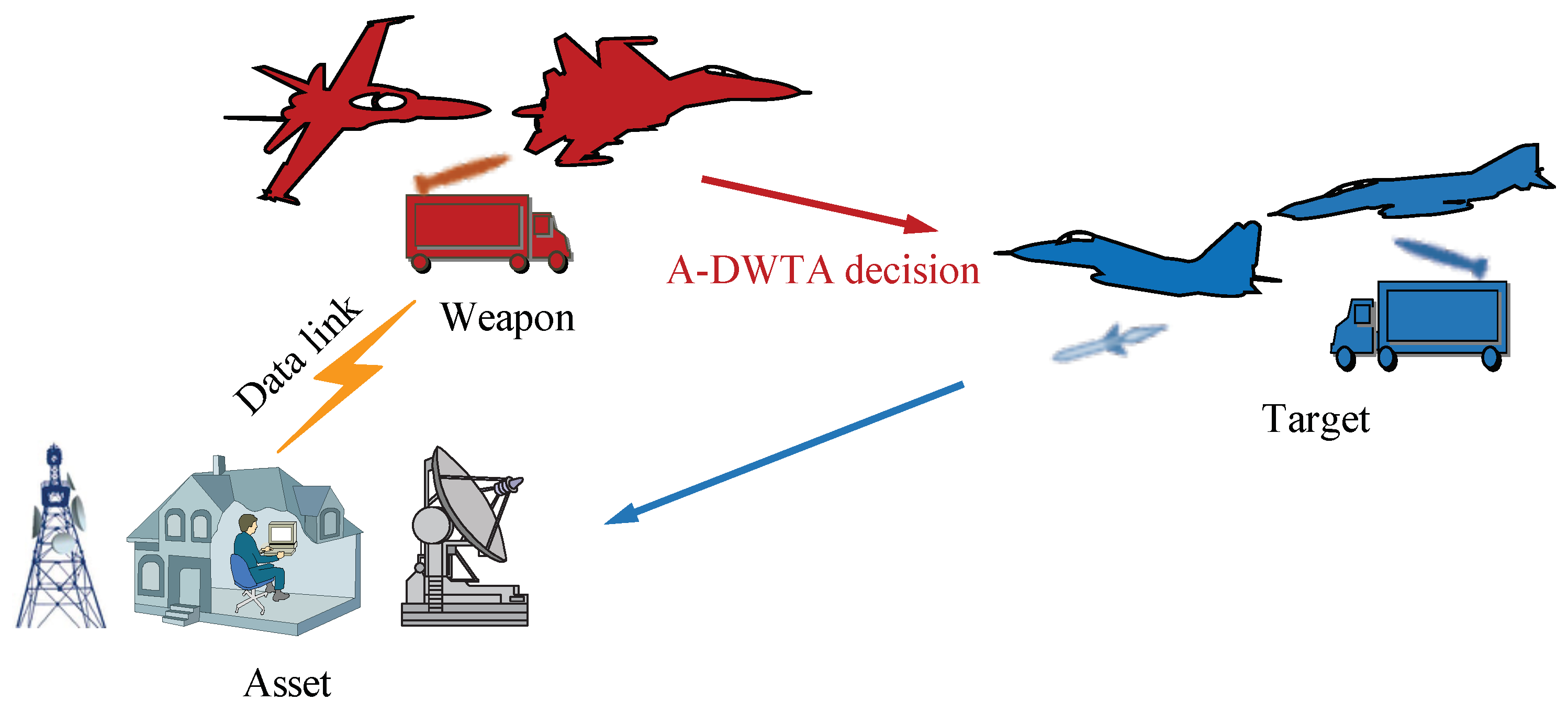
:1. Introduction
- An OODA/A-DWTA loop model is established for supporting the following A-DWTA decision model and solving algorithm.
- To reflect the actual operational requirement, an A-DWTA decision model based on the receding horizon strategy is presented. The “radical–conservative” degree of the obtained plan, which relates to the number of decision stages, can be adaptively adjusted by the model parameter.
- A heuristic algorithm based on statistical marginal return is proposed to solve the A-DWTA model, which has the advantage of robust and real-time. The extensive experiments demonstrate the effectiveness of the proposed approaches.
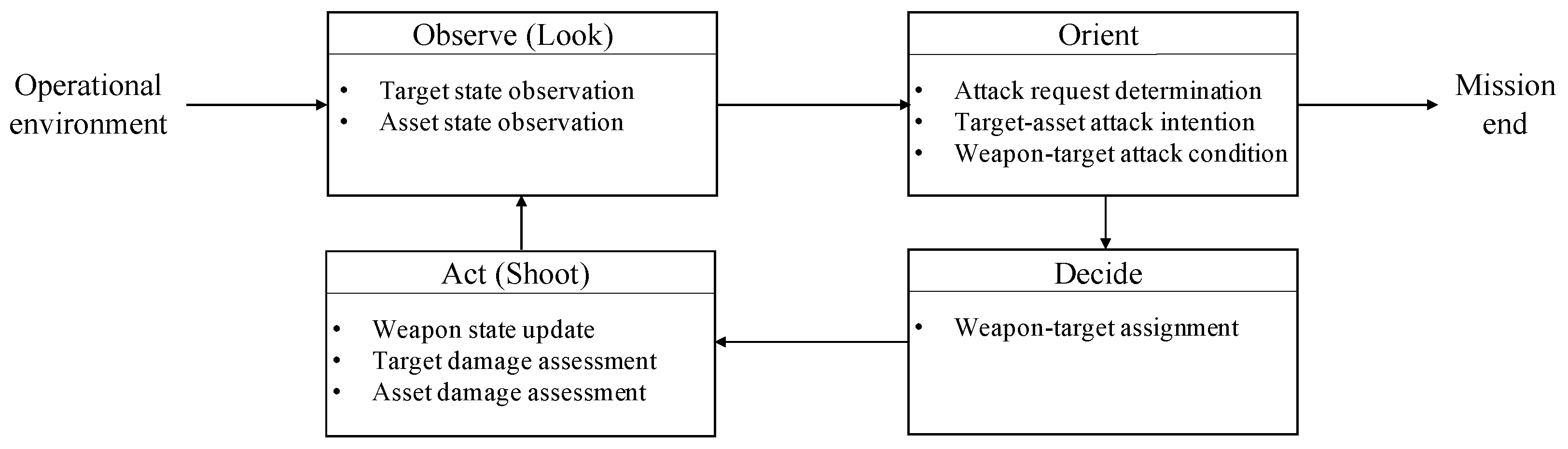
2. Ooda/A-Dwta Loop Model
2.1. Observe Phase
- (1)
- Target state observation. Let the current stage be s, and the target observed state is the actual survival state of targets after the act phase of stage . Therefore, the observed target state at stage s should follow the Bernoulli distribution about the target survival probability at stage , namely ∼:where indicates that the observed state of the target j in observation phase is damaged; conversely, represents target j as a threat target in observation phase; is the target survival probability expectation after the end of stage , which is given in the damage assessment of the act phase.
- (2)
- Asset state observation. Similarly, the asset observed state of stage s follows the Bernoulli distribution of the asset survival probability expectation of stage . The asset survival probability expectation is related to the target survival probability expectation in the act phase of stage , and the target observed state can be obtained in the stage s. Therefore, in the observation model of OODA/A-DWTA, the asset survival probability expectation of stage is modeled as the posterior conditional probability of the target observed state of stage s:
2.2. Orient Phase
- (1)
- Attack request determination. When any of the following conditions are met, the OODA/A-DWTA loop terminates, otherwise initiates an attack request and enters the decide phase: (a) all assets are destroyed, , where is the l1-norm; (b) all targets are damaged, ; (c) no available weapon, . So the termination condition of OODA/A-DWTA is .
- (2)
- Target–asset attack intention. In actual combat, the identification of enemy target’s attack intention requires the analysis of target altitude, distance, speed, acceleration, heading angle, azimuth, fire control radar state, maneuver type, and is predicted by domain knowledge. WTA research’s focus lies in the decision model and algorithm of the command and control layer, not the methods of intention recognition. Hence we simplify the target-asset intention matrix to describe the enemy targets’ attack state of each stage. represents that the attack intention of target j against asset k is not recognized at stage s. Otherwise, it represents that target j against asset k, and the destroy probability is .
- (3)
- Weapon–target attack condition. The condition of weapon–target attack is mainly determined by whether the time window of the fire control launch is satisfied. In DWTA, as the offensive and defensive stages recurse, the weapons that meet the attack conditions usually decrease. We introduce the lethality matrix and feasibility matrix to describe the weapon-target attack condition of each stage, where represents the destroy probability of weapon i against target j; indicates that weapon i meets the attack condition of intercepting target j, otherwise .
2.3. Decide Phase
2.4. Act Phase
- (1)
- Weapon state update. After acting the weapon allocation plan, the current stage’s weapon state are determined by the previous stage’s weapon states and the current stage’s decision plan .where denotes weapon i is not available at stage s, otherwise .
- (2)
- Target damage assessment. The target survival probability is mainly determined by the target state, the weapon–target kill probability and the decision plan at current stage.where (6), . If and only if , that is, the target j is confirmed as damaged by the observe phase of the stage s, ; if and only if and , that is, no weapon is not assigned to the target j with threat capability, .
- (3)
- Asset damage assessment. The asset survival value expectation of stage s is related to the asset value and the asset survival probability expectation in the act phase of stage s. In the act model of OODA/A-DWTA, the asset survival probability expectation of stage s is modelled as the conditional probability under the target survival probabilitywhere the term represents the damage probability of target j attacking asset k in the act phase of stage s. The asset survival value expectation is evaluated aswhere . If and only if , that is, the asset k is confirmed as destroyed by the observe phase of the stage s, ; if and only if and , that is, no target has attack intention to the target j, .
3. A-Dwta/Rh Formulation
3.1. Objective Building
3.1.1. Absolute Return Expectation at the Current Stage
3.1.2. Return Evaluation of Remaining Weapons on Prediction Situation
3.2. Constraints
4. Ha-Smr Algorithm
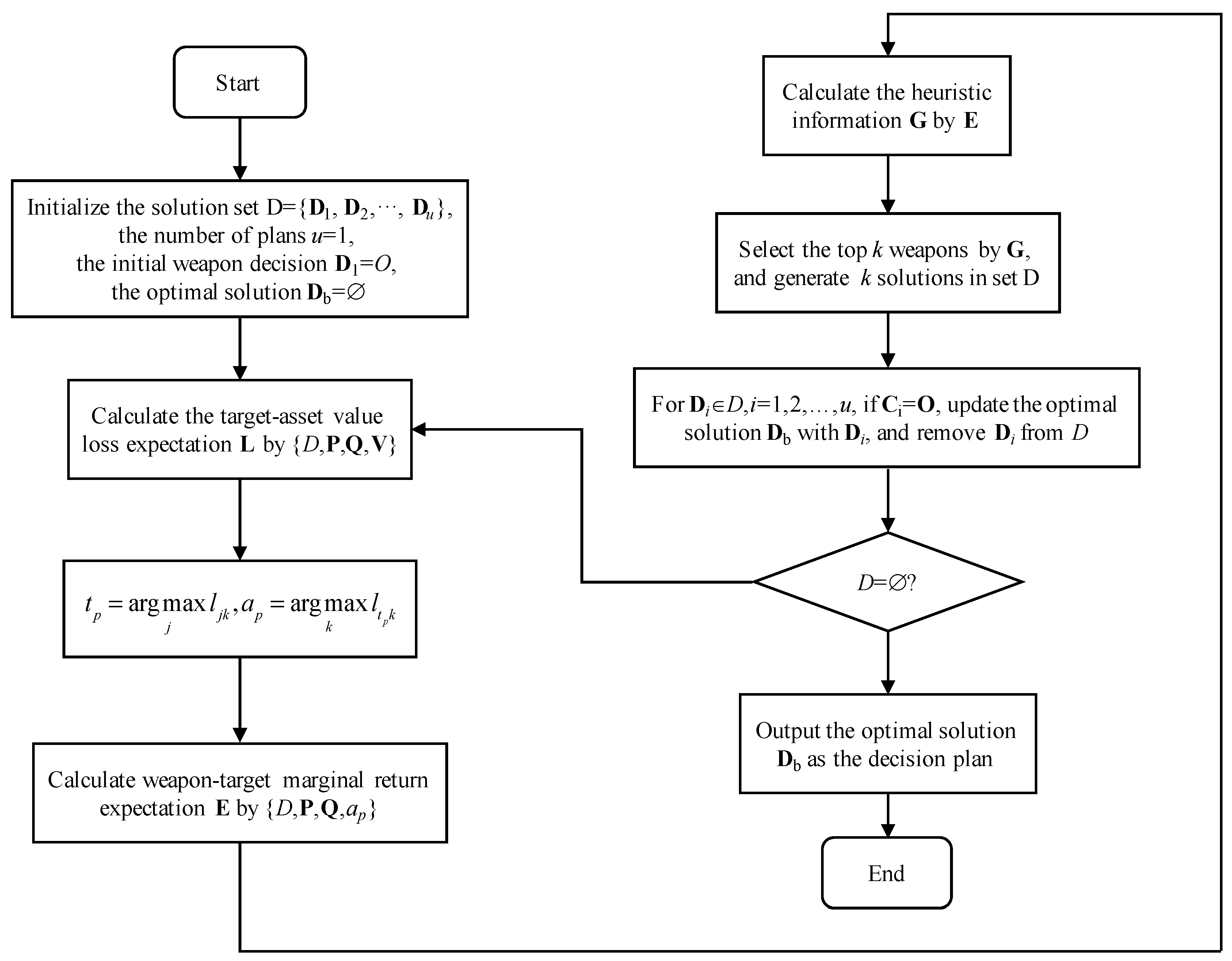
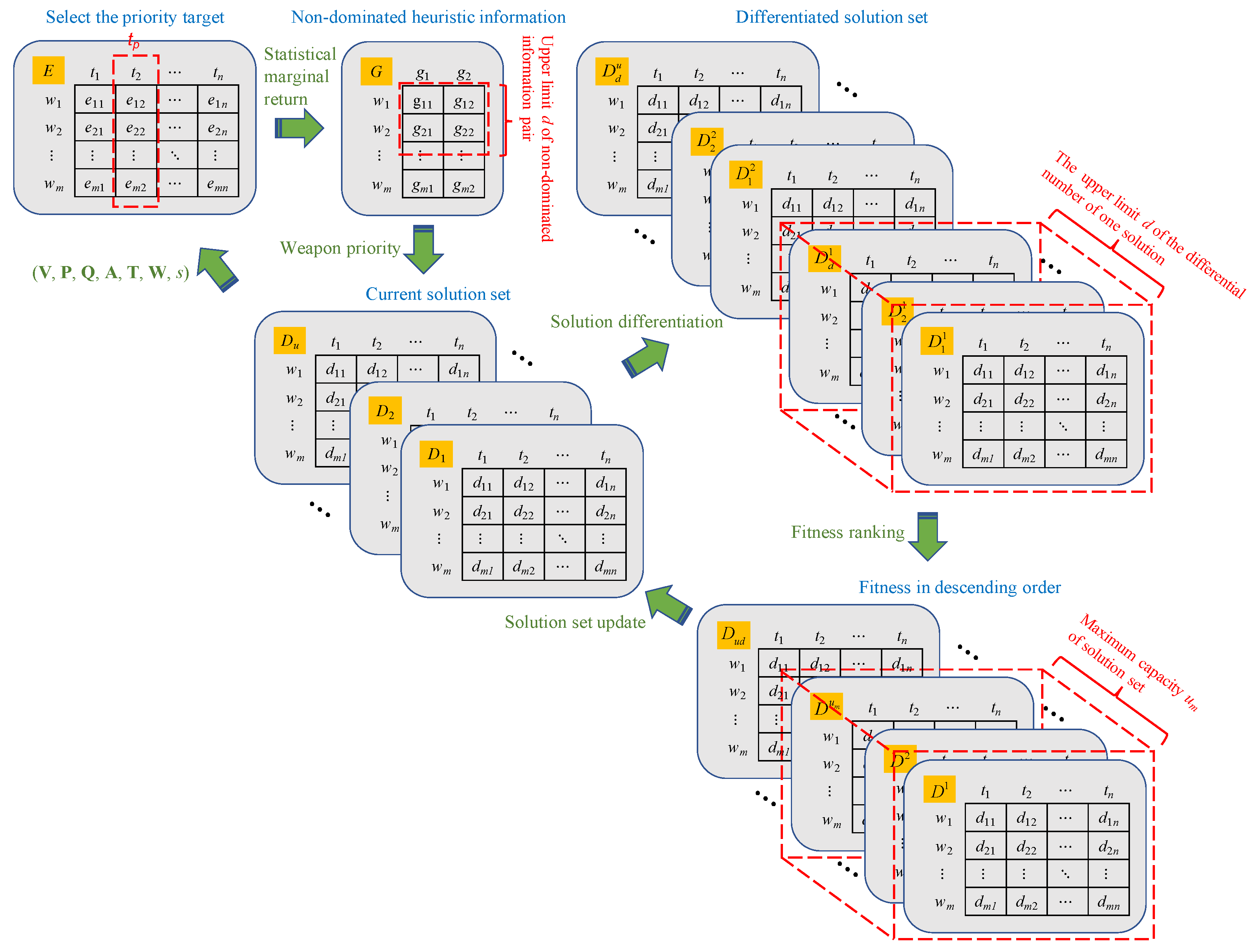
4.1. Algorithm Framework
| Algorithm 1. Main loop of heuristic algorithm based on statistical marginal return (HA-SMR). |
|
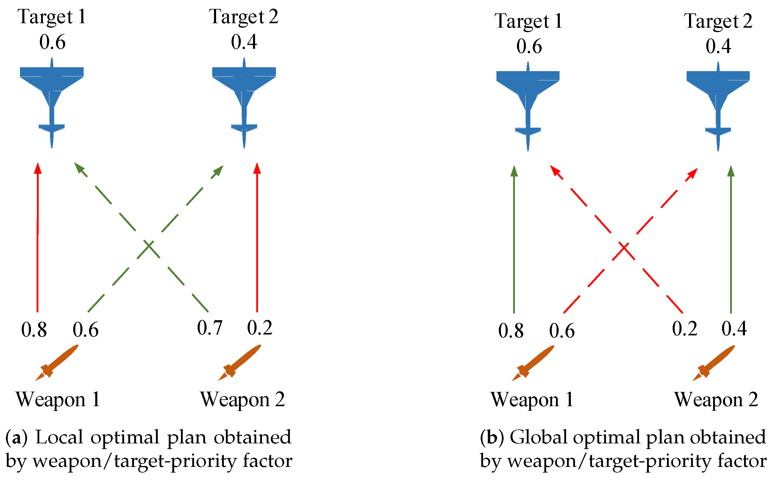
4.1.1. Priority of Target and Asset
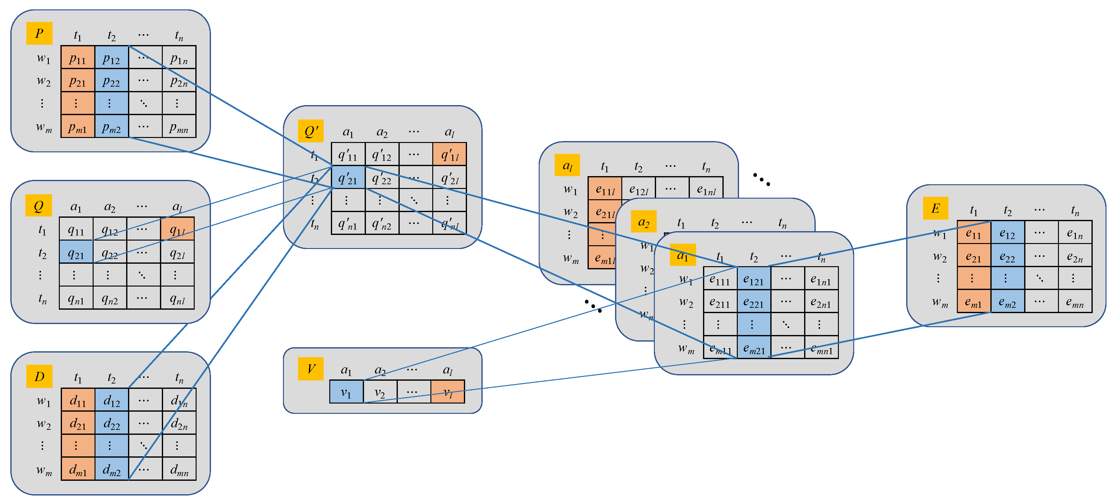
4.1.2. Weapon–Target Marginal Return Expectation
4.2. Heuristic Information Design
4.3. Constraint Handling
5. Experimental Studies
5.1. Operational Scenario and Performance Metrics
- (1)
- Target–asset destroy intention. Assuming that the defender is unknown to the targets’ attack strategy, and the threat assessment system identifies the target intention. The initialization method of target–asset destroy matrix is: (i) when targets are no fewer than assets (), the target intension is generated randomly on the premise that each asset is assigned at least one target. (ii) When there are more targets than assets (), the target intension is generated randomly under the premise that each target aims to different assets. The target–asset destroy probability is initialized aswhere and reflect the upper and lower bounds of target-asset vulnerability.
- (2)
- Weapon–target attack condition. The weapon-target kill probability is initialized bywhere and denotes the upper and lower bounds of weapon-target kill probability. In the evolution of subsequent stages, due to the operational state’s continuity, the weapon–target kill matrix of the current stage should be related to the weapon–target kill matrix, weapon state and target state of the previous stage. Let the transfer state of weapon–target kill probability follow
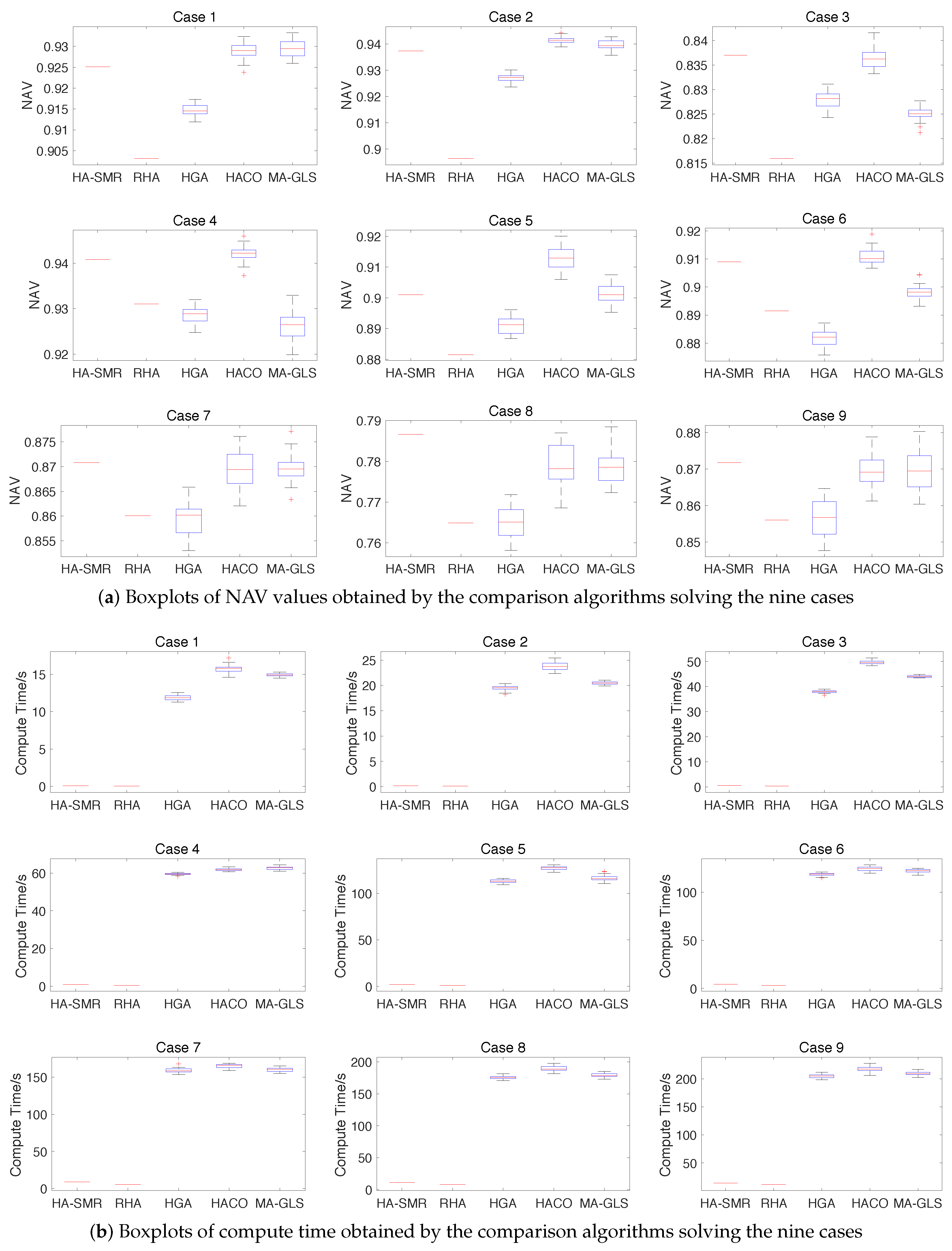
5.2. Experiments on Comparison Algorithms
- A-DWTA/RH model: the weight of the absolute return expectation at the current stage = 0.6; the weight of the retun evaluation of remaining weapons on prediction situation = 1 − = 0.4;
- HA-SMR: The capacity of solution set = 50; the differentiation number d = 4; the threshold of weapon consumption = 0.85;
- HGA: the population size = 100; the number of elite individuals = 100; the crossover probability = 0.8; the mutation probability = 0.2;
- HACO: the population size = 200; the train importance factor = 1; the visibility importance factor = 2; the pheromone evaporation rate = 0.5;
- MA-GLS: the population size = 200; the crossover/mutation number of each generation is set to 10.
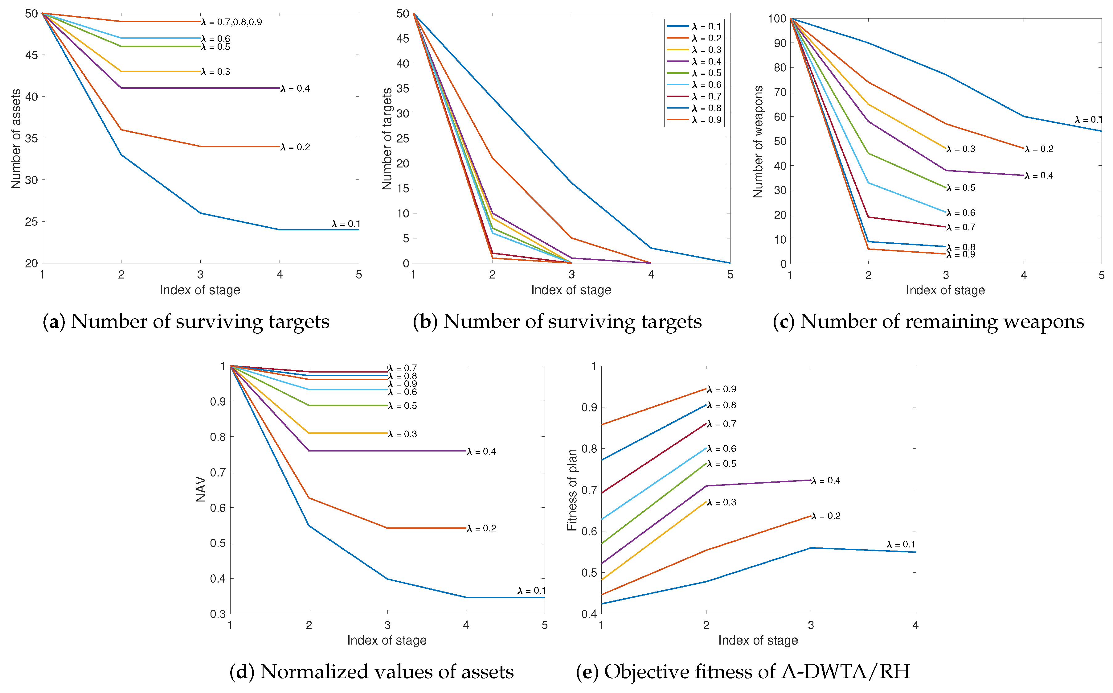
5.3. Parameter Sensitivity
5.3.1. Model Weight
- All assets are destroyed (), defense mission fails, let .
- Assets are not all damaged and targets are all killed ( and ), the defense task is completed, let .
- Assets have not been destroyed and targets have not been killed, but weapons have been consumed (, and ). It is predicted that the defense mission will fail, and let .
5.3.2. Problem Scale
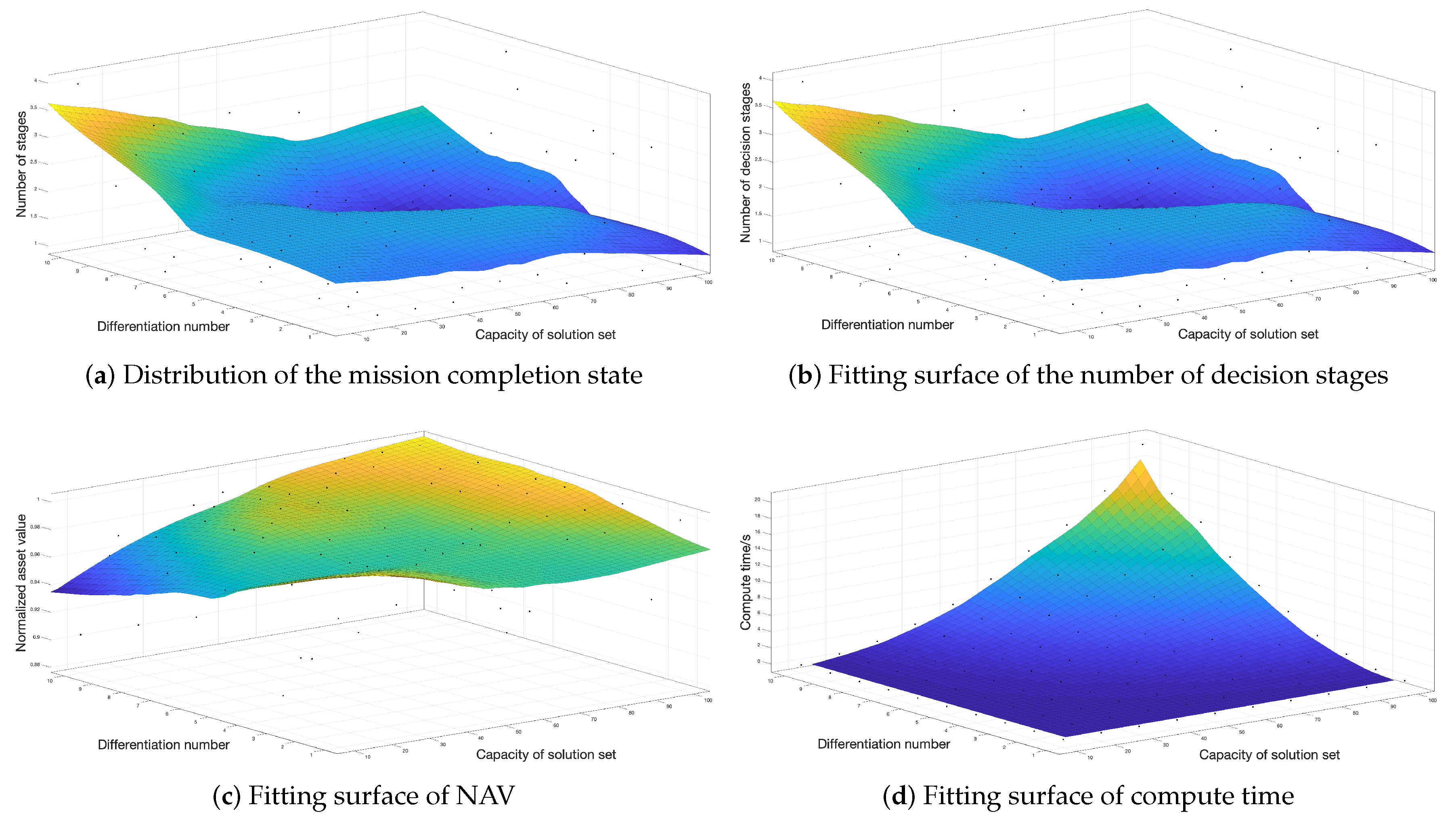
5.3.3. Set Capacity and Differentiation Number D
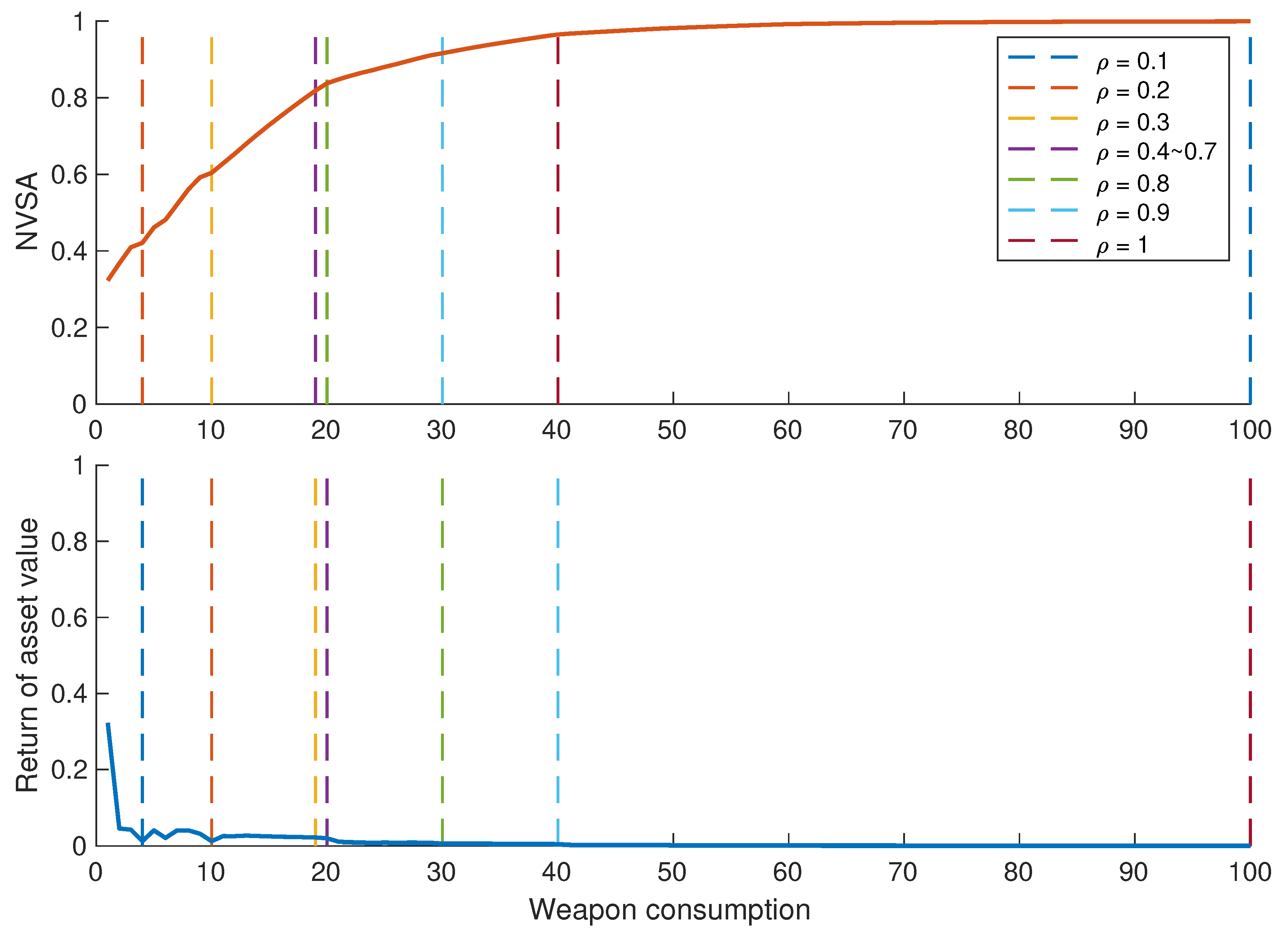
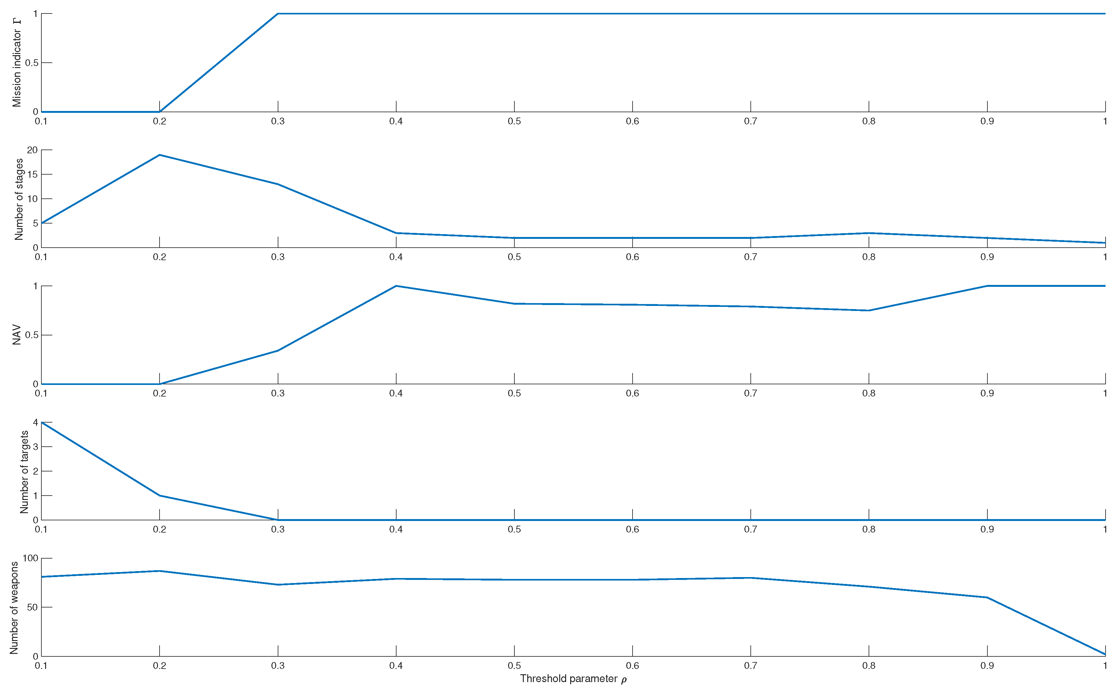
5.3.4. Threshold Parameter
6. Conclusions and Future Work
Author Contributions
Funding
Acknowledgments
Conflicts of Interest
References
- Roux, J.N.; Van Vuuren, J.H. Threat evaluation and weapon assignment decision support: A review of the state of the art. ORiON 2007, 23, 151–187. [Google Scholar] [CrossRef] [Green Version]
- Yang, Z.; Zhou, D.; Kong, W.; Piao, H.; Zhang, K.; Zhao, Y. Nondominated Maneuver Strategy Set with Tactical Requirements for a Fighter Against Missiles in a Dogfight. IEEE Access 2020, 8, 117298–117312. [Google Scholar] [CrossRef]
- Manne, A.S. A target-assignment problem. Oper. Res. 1958, 6, 346–351. [Google Scholar] [CrossRef]
- Hosein, P.A.; Athans, M. Preferential Defense Strategies. Part I: The Static Case; this Issue. 1990. Available online: https://core.ac.uk/download/pdf/4378993.pdf (accessed on 14 September 2020).
- Hosein, P.; Athans, M. Preferential Defense Strategies. Part 2: The Dynamic Case; LIDS-P-2003; MIT: Cambridge, MA, USA, 1990. [Google Scholar]
- Cai, H.; Liu, J.; Chen, Y.; Wang, H. Survey of the research on dynamic weapon-target assignment problem. J. Syst. Eng. Electron. 2006, 17, 559–565. [Google Scholar]
- Zhang, K.; Zhou, D.; Yang, Z.; Pan, Q.; Kong, W. Constrained Multi-Objective Weapon Target Assignment for Area Targets by Efficient Evolutionary Algorithm. IEEE Access 2019, 7, 176339–176360. [Google Scholar] [CrossRef]
- Murphey, R.A. Target-based weapon target assignment problems. In Nonlinear Assignment Problems; Springer: Berlin, Germany, 2000; pp. 39–53. [Google Scholar]
- Cho, D.H.; Choi, H.L. Greedy Maximization for Asset-Based Weapon-Target Assignment with Time-Dependent Rewards. Coop. Control Multi-Agent Syst. Theory Appl. 2017, 115–139. Available online: https://onlinelibrary.wiley.com/doi/10.1002/9781119266235.ch5 (accessed on 14 September 2020).
- Xin, B.; Wang, Y.; Chen, J. An efficient marginal-return-based constructive heuristic to solve the sensor– weapon–target assignment problem. IEEE Trans. Syst. Man Cybern. Syst. 2018, 49, 2536–2547. [Google Scholar] [CrossRef]
- Li, X.; Zhou, D.; Yang, Z.; Pan, Q.; Huang, J. A novel genetic algorithm for the synthetical Sensor-Weapon-Target assignment problem. Appl. Sci. 2019, 9, 3803. [Google Scholar] [CrossRef] [Green Version]
- Kline, A.; Ahner, D.; Hill, R. The weapon-target assignment problem. Comput. Oper. Res. 2019, 105, 226–236. [Google Scholar] [CrossRef]
- Hosein, P.A.; Athans, M. Some Analytical Results for the Dynamic Weapon-Target Allocation Problem; Technical Report; Massachusetts Inst of Tech Cambridge Lab for Information and Decision Systems: Cambridge, MA, USA, 1990. [Google Scholar]
- Eckler, A.R.; Burr, S.A. Mathematical Models of Target Coverage and Missile Allocation; Technical Report; Military Operations Research Society: Alexandria, VA, USA, 1972. [Google Scholar]
- Soland, R.M. Optimal terminal defense tactics when several sequential engagements are possible. Oper. Res. 1987, 35, 537–542. [Google Scholar] [CrossRef]
- Hosein, P.; Athans, M. The Dynamic Weapon-Target Assignment Problem; Technical Report; 1989; Available online: https://core.ac.uk/download/pdf/4380801.pdf (accessed on 14 September 2020).
- Leboucher, C.; Shin, H.S.; Siarry, P.; Chelouah, R.; Le Ménec, S.; Tsourdos, A. A two-step optimisation method for dynamic weapon target assignment problem. In Recent Advances on Meta-Heuristics and Their Application to Real Scenarios; InTech: Rijeka, Crotia, 2013; pp. 109–129. [Google Scholar]
- Zhengrong, J.; Faxing, L.; Hangyu, W. Multi-stage attack weapon target allocation method based on defense area analysis. J. Syst. Eng. Electron. 2020, 31, 539–550. [Google Scholar] [CrossRef]
- Jang, J.; Yoon, H.G.; Kim, J.C.; Kim, C.O. Adaptive Weapon-to-Target Assignment Model Based on the Real-Time Prediction of Hit Probability. IEEE Access 2019, 7, 72210–72220. [Google Scholar] [CrossRef]
- Lloyd, S.P.; Witsenhausen, H.S. Weapons allocation is NP-complete. In Proceedings of the 1986 Summer Computer Simulation Conference, Reno, NV, USA, 28–30 July 1986; pp. 1054–1058. [Google Scholar]
- Hocaoğlu, M.F. Weapon target assignment optimization for land based multi-air defense systems: A goal programming approach. Comput. Ind. Eng. 2019, 128, 681–689. [Google Scholar] [CrossRef]
- Cao, M.; Fang, W. Swarm Intelligence Algorithms for Weapon-Target Assignment in a Multilayer Defense Scenario: A Comparative Study. Symmetry 2020, 12, 824. [Google Scholar] [CrossRef]
- Kline, A.G.; Ahner, D.K.; Lunday, B.J. Real-time heuristic algorithms for the static weapon target assignment problem. J. Heuristics 2019, 25, 377–397. [Google Scholar] [CrossRef]
- Zhao, P.; Wang, J.; Kong, L. Decentralized Algorithms for Weapon-Target Assignment in Swarming Combat System. Math. Probl. Eng. 2019, 2019, 8425403. [Google Scholar] [CrossRef]
- Summers, D.S.; Robbins, M.J.; Lunday, B.J. An approximate dynamic programming approach for comparing firing policies in a networked air defense environment. Comput. Oper. Res. 2020, 117, 104890. [Google Scholar] [CrossRef]
- Fu, G.; Wang, C.; Zhang, D.; Zhao, J.; Wang, H. A Multiobjective Particle Swarm Optimization Algorithm Based on Multipopulation Coevolution for Weapon-Target Assignment. Math. Probl. Eng. 2019, 2019, 1424590. [Google Scholar] [CrossRef]
- Guo, D.; Liang, Z.; Jiang, P.; Dong, X.; Li, Q.; Ren, Z. Weapon-target assignment for multi-to-multi interception with grouping constraint. IEEE Access 2019, 7, 34838–34849. [Google Scholar] [CrossRef]
- Chen, J.; Xin, B.; Peng, Z.; Dou, L.; Zhang, J. Evolutionary decision-makings for the dynamic weapon-target assignment problem. Sci. China Ser. F Inf. Sci. 2009, 52, 2006. [Google Scholar] [CrossRef]
- Chang, T.; Kong, D.; Hao, N.; Xu, K.; Yang, G. Solving the dynamic weapon target assignment problem by an improved artificial bee colony algorithm with heuristic factor initialization. Appl. Soft Comput. 2018, 70, 845–863. [Google Scholar] [CrossRef]
- Wang, Y.; Li, J.; Huang, W.; Wen, T. Dynamic weapon target assignment based on intuitionistic fuzzy entropy of discrete particle swarm. China Commun. 2017, 14, 169–179. [Google Scholar] [CrossRef]
- Lai, C.M.; Wu, T.H. Simplified swarm optimization with initialization scheme for dynamic weapon–target assignment problem. Appl. Soft Comput. 2019, 82, 105542. [Google Scholar] [CrossRef]
- Shin, M.K.; Lee, D.; Choi, H.L. Weapon-Target Assignment Problem with Interference Constraints using Mixed-Integer Linear Programming. arXiv 2019, arXiv:1911.12567. [Google Scholar]
- Lee, D.; Shin, M.K.; Choi, H.L. Weapon Target Assignment Problem with Interference Constraints. In Proceedings of the AIAA Scitech 2020 Forum, Orlando, FL, USA, 6–10 January 2020; p. 0388. [Google Scholar]
- Xu, W.; Chen, C.; Ding, S.; Pardalos, P.M. A bi-objective dynamic collaborative task assignment under uncertainty using modified MOEA/D with heuristic initialization. Exp. Syst. Appl. 2020, 140, 112844. [Google Scholar] [CrossRef]
- Ahuja, R.K.; Kumar, A.; Jha, K.; Orlin, J.B. Exact and Heuristic Methods for the Weapon Target Assignment Problem; INFORMS: Catonsville, MD, USA, 2003. [Google Scholar]
- Lee, Z.J.; Su, S.F.; Lee, C.Y. Efficiently solving general weapon-target assignment problem by genetic algorithms with greedy eugenics. IEEE Trans. Syst. Man Cybern. Part B Cybern. 2003, 33, 113–121. [Google Scholar]
- Xin, B.; Chen, J.; Peng, Z.; Dou, L.; Zhang, J. An efficient rule-based constructive heuristic to solve dynamic weapon-target assignment problem. IEEE Trans. Syst. Man Cybern.-Part A Syst. Hum. 2010, 41, 598–606. [Google Scholar] [CrossRef] [Green Version]
- Leboucher, C.; Shin, H.; Le Ménec, S.; Tsourdos, A.; Kotenkoff, A. Optimal weapon target assignment based on an geometric approach. IFAC Proc. Vol. 2013, 46, 341–346. [Google Scholar] [CrossRef]
- Leboucher, C.; Shin, H.S.; Le Ménec, S.; Tsourdos, A.; Kotenkoff, A.; Siarry, P.; Chelouah, R. Novel evolutionary game based multi-objective optimisation for dynamic weapon target assignment. IFAC Proc. Vol. 2014, 47, 3936–3941. [Google Scholar] [CrossRef] [Green Version]
- Li, J.; Chen, J.; Xin, B.; Dou, L. Solving multi-objective multi-stage weapon target assignment problem via adaptive NSGA-II and adaptive MOEA/D: A comparison study. In Proceedings of the 2015 IEEE Congress on Evolutionary Computation (CEC), Sendai, Japan, 25–28 May 2015; pp. 3132–3139. [Google Scholar]
- Li, J.; Chen, J.; Xin, B.; Dou, L.; Peng, Z. Solving the uncertain multi-objective multi-stage weapon target assignment problem via MOEA/D-AWA. In Proceedings of the 2016 IEEE Congress on Evolutionary Computation (CEC), Vancouver, BC, Canada, 24–29 July 2016; pp. 4934–4941. [Google Scholar]
- Li, J.; Chen, J.; Xin, B.; Chen, L. Efficient multi-objective evolutionary algorithms for solving the multi-stage weapon target assignment problem: A comparison study. In Proceedings of the 2017 IEEE Congress on Evolutionary Computation (CEC), San Sebastian, Spain, 5–8 June 2017; pp. 435–442. [Google Scholar]
- Li, J.; Chen, J.; Xin, B. Optimizing multi-objective uncertain multi-stage weapon target assignment problems with the risk measure CVaR. In Proceedings of the 2019 IEEE 15th International Conference on Control and Automation (ICCA), Edinburgh, UK, 16–19 July 2019; pp. 61–66. [Google Scholar]
- Mei, Z.; Peng, Z.; Zhang, X. Optimal dynamic weapon-target assignment based on receding horizon control heuristic. In Proceedings of the 2017 13th IEEE International Conference on Control & Automation (ICCA), Ohrid, Macedonia, 3–6 July 2017; pp. 876–881. [Google Scholar]
- Kalyanam, K.; Casbeer, D.; Pachter, M. Monotone optimal threshold feedback policy for sequential weapon target assignment. J. Aerosp. Inf. Syst. 2017, 14, 68–72. [Google Scholar] [CrossRef]
- Duan, W.; Yuan, W.; Pan, L. Research on Algorithm for Dynamic Weapon Target Assignment Based on the Improved Markov Decision Model. In Proceedings of the 2018 37th Chinese Control Conference (CCC), Wuhan, China, 25–27 July 2018; pp. 8417–8424. [Google Scholar]


| Notation | Description |
|---|---|
| m | the number of available weapons at the initial stage; |
| n | the number of hostile targets at the initial stage; |
| l | the number of defense asset at the initial stage; |
| s | the index of decision stage, ; |
| the weapon state of stage s; denotes weapon i is available at the decide phase of stage s, otherwise ; | |
| the target state of stage s; denotes target j is threatening at the observe phase of stage s, otherwise ; | |
| the asset state of stage s; denotes asset k survives at the observe phase of stage s, otherwise ; | |
| the weapon–target kill probability of stage s, denotes the kill probability of weapon i against target j at the orient phase of stage s; | |
| the weapon=target attack condition of stage s; indicates that weapon i satisfies the attack condition of intercepting target j at stage s, otherwise ; | |
| the target–asset intention matrix of stage s; denotes that the attack intention of target j against asset k is assessed at the orient phase of stage s, and the destroy probability is , otherwise ; | |
| the weapon–target decision variable of stage s; represents that weapon i is assigned to intercept target j at the decide phase of stage s, otherwise ; | |
| the target survival probability after the act phase of stage s; | |
| the asset survival probability at the observe phase of stage s; | |
| the asset survival probability after the act phase of stage s. |
| Scale | No.1 | No.2 | No.3 | No.4 | No.5 | No.6 | No.7 | No.8 | No.9 |
|---|---|---|---|---|---|---|---|---|---|
| m | 28 | 35 | 69 | 81 | 105 | 114 | 137 | 136 | 159 |
| n | 18 | 21 | 36 | 47 | 58 | 65 | 72 | 82 | 97 |
| l | 13 | 24 | 48 | 62 | 80 | 55 | 91 | 77 | 58 |
| Case | Mean Metric | Comparison Algorithms | ||||
|---|---|---|---|---|---|---|
| HA-SMR | RHA | HGA | HACO | MA-GLS | ||
| No.1 | NAV | 0.9251 ± 0 | 0.9013 ± 0 | 0.9301 ± 0.0014 | 0.9295 ± 0.0017 | 0.9147 ± 0.0019 |
| CT | 0.07 ± 0 | 0.03 ± 0 | 11.84 ± 0.37 | 15.83 ± 0.52 | 14.93 ± 0.22 | |
| No.2 | NAV | 0.9374 ± 0 | 0.8963 ± 0 | 0.9398 ± 0.0017 | 0.9416 ± 0.0013 | 0.9262 ± 0.0016 |
| CT | 0.15 ± 0 | 0.09 ± 0 | 19.39 ± 0.54 | 23.85 ± 0.78 | 20.39 ± 0.46 | |
| No.3 | NAV | 0.8370 ± 0 | 0.8359 ± 0 | 0.8352 ± 0.0020 | 0.8364 ± 0.0019 | 0.8284 ± 0.0015 |
| CT | 0.50 ± 0 | 0.28 ± 0 | 37.98 ± 0.55 | 49.56 ± 0.61 | 43.98 ± 0.50 | |
| No.4 | NAV | 0.9408 ± 0 | 0.9268 ± 0 | 0.9385 ± 0.0018 | 0.9417 ± 0.0021 | 0.9201 ± 0.0027 |
| CT | 0.96 ± 0 | 0.52 ± 0 | 59.46 ± 0.54 | 61.93 ± 0.72 | 62.87 ± 0.79 | |
| No.5 | NAV | 0.9010 ± 0 | 0.8815 ± 0 | 0.8905 ± 0.0028 | 0.9118 ± 0.0035 | 0.9007 ± 0.0033 |
| CT | 1.87 ± 0 | 1.16 ± 0 | 113.06 ± 1.49 | 126.65 ± 1.81 | 115.48 ± 2.36 | |
| No.6 | NAV | 0.9090 ± 0 | 0.8915 ± 0 | 0.8972 ± 0.0038 | 0.9107 ± 0.0030 | 0.8906 ± 0.0031 |
| CT | 4.27 ± 0 | 3.22 ± 0 | 117.79 ± 1.96 | 124.66 ± 2.04 | 121.90 ± 1.72 | |
| No.7 | NAV | 0.8708 ± 0 | 0.8611 ± 0 | 0.8635 ± 0.0036 | 0.8815 ± 0.0034 | 0.8783 ± 0.0037 |
| CT | 8.91 ± 0 | 5.52 ± 0 | 158.97 ± 2.96 | 165.49 ± 3.14 | 159.42 ± 2.92 | |
| No.8 | NAV | 0.7866 ± 0 | 0.7619 ± 0 | 0.7652 ± 0.0039 | 0.7710 ± 0.0041 | 0.7553 ± 0.0045 |
| CT | 11.29 ± 0 | 8.11 ± 0 | 176.10 ± 2.58 | 189.55 ± 3.96 | 178.96 ± 3.16 | |
| No.8 | NAV | 8718 ± 0 | 0.8340 ± 0 | 0.8379 ± 0.0043 | 0.8651 ± 0.0047 | 0.8492 ± 0.0048 |
| CT | 14.23 ± 0 | 11.57 ± 0 | 205.96 ± 3.81 | 217.91 ± 4.13 | 209.91 ± 3.63 | |
| Parameter | Stage | Compute Time | NAV | Plan Fitness | Termination State |
|---|---|---|---|---|---|
| 0.1 | 4 | 3.3302 | 0.3461 | 0.5391 | Γ1:W54T0A24 |
| 0.2 | 3 | 1.9247 | 0.5417 | 0.6369 | Γ1:W47T0A34 |
| 0.3 | 2 | 1.7992 | 0.8096 | 0.6713 | Γ1:W47T0A43 |
| 0.4 | 3 | 1.8254 | 0.7599 | 0.7235 | Γ1:W36T0A41 |
| 0.5 | 2 | 1.4043 | 0.8882 | 0.7640 | Γ1:W31T0A46 |
| 0.6 | 2 | 1.6805 | 0.9328 | 0.8012 | Γ1:W21T0A47 |
| 0.7 | 2 | 1.2787 | 0.9832 | 0.8604 | Γ1:W15T0A49 |
| 0.8 | 2 | 1.3525 | 0.9721 | 0.9057 | Γ1:W7T0A49 |
| 0.9 | 2 | 1.2706 | 0.9615 | 0.9448 | Γ1:W4T0A49 |
© 2020 by the authors. Licensee MDPI, Basel, Switzerland. This article is an open access article distributed under the terms and conditions of the Creative Commons Attribution (CC BY) license (http://creativecommons.org/licenses/by/4.0/).
Share and Cite
Zhang, K.; Zhou, D.; Yang, Z.; Zhao, Y.; Kong, W. Efficient Decision Approaches for Asset-Based Dynamic Weapon Target Assignment by a Receding Horizon and Marginal Return Heuristic. Electronics 2020, 9, 1511. https://doi.org/10.3390/electronics9091511
Zhang K, Zhou D, Yang Z, Zhao Y, Kong W. Efficient Decision Approaches for Asset-Based Dynamic Weapon Target Assignment by a Receding Horizon and Marginal Return Heuristic. Electronics. 2020; 9(9):1511. https://doi.org/10.3390/electronics9091511
Chicago/Turabian StyleZhang, Kai, Deyun Zhou, Zhen Yang, Yiyang Zhao, and Weiren Kong. 2020. "Efficient Decision Approaches for Asset-Based Dynamic Weapon Target Assignment by a Receding Horizon and Marginal Return Heuristic" Electronics 9, no. 9: 1511. https://doi.org/10.3390/electronics9091511