ST-TrafficNet: A Spatial-Temporal Deep Learning Network for Traffic Forecasting

Abstract

This paper presents a spatial-temporal deep learning network, termed ST-TrafficNet, for traffic flow forecasting. Recent deep learning methods highly relate accurate predetermined graph structure for the complex spatial dependencies of traffic flow, and ineffectively harvest high dimensional temporal features of the traffic flow. In this paper, a novel multi-diffusion convolution block constructed by an attentive diffusion convolution and bidirectional diffusion convolution is proposed, which is capable to extract precise potential spatial dependencies. Moreover, a stacked Long Short-Term Memory (LSTM) block is adopted to capture high-dimensional temporal features. By integrating the two blocks, the ST-TrafficNet can learn the spatial-temporal dependencies of intricate traffic data accurately. The performance of the ST-TrafficNet has been evaluated on two real-world benchmark datasets by comparing it with three commonly-used methods and seven state-of-the-art ones. The Mean Absolute Error (MAE), Root Mean Square Error (RMSE), and Mean Absolute Percentage Error (MAPE) of the proposed method outperform not only the commonly-used methods, but also the state-of-the-art ones in 15 min, 30 min, and 60 min time-steps.

1. Introduction

With the advance of intelligent transportation systems (ITSs), traffic forecasting has received increasing attention since accurate traffic forecasting plays a significant role in various ITSs, including traffic signal control system [1], navigation system [2], and route guidance system [3].

The goal of traffic forecasting is to forecast the traffic conditions (e.g., traffic flow and speed) of several future time-steps given the historic traffic data [4]. However, the task is challenging due to the natural complexity and uncertainty of traffic patterns. As shown in Figure 1, many loop sensors are planted under the roads, and the function of them is to collect traffic data by detecting every passing vehicle. Then, the traffic data of the entire traffic network are sampled as traffic graph signals. Each node of the traffic network graph represents a sensor and the signals of the node are the traffic data records. On the one hand, the nodes in the same traffic stream are related to each other, for instance, the pattern of upstream node signals will appear soon in the downstream node signals. Moreover, the continuous node signals have seasonality and trend, which means the patterns of weekday are similar to each other while different from the patterns of weekend and the trend of vehicle number is rising year by year. Both the spatial and temporal features are important to traffic forecasting, and one main idea of traffic forecasting is to extract spatial-temporal dependencies of historic traffic graph signals to learn traffic patterns and make accurate predictions.

Recently, researchers propose to integrate Convolutional Neural Network (CNN) or Graph Convolutional Network (GCN) to Recurrent Neural Network (RNN) or Long Short-Term Memory (LSTM) to simultaneously explore the spatial-temporal relationships inside the traffic flow data [5,6,7,8]. However, such methods face two major shortcomings. First, the GCN-based approaches require a predetermined graph structure, which is constructed based on human knowledge or a simple algorithm using the distance from node to node [6], and assume it reflects the genuine spatial dependencies of the whole traffic network. However, the predetermined graph structure could have mistakes under several conditions. For instance, as shown in Figure 1, nodes 1 and 2 could be connected due to the short-distance but they are not spatially related since they are planted in opposite direction carriageways, nodes 2 and 5 could have no correspondence in the graph because of the long-distance but they are in the same traffic stream and highly related. Furthermore, the traffic flow is not only affected by the property of a road network, such as the number of lanes or the slope of the pavement, but also the social circumstances near the road segment. The social circumstances include a series of interactional characteristics, such as the economics of the area, the demographic density, the territorial functions, etc. The economics of the area, or the demographic are difficult to be quantitatively defined in a traffic graph structure. In this regard, a predefined graph structure that only considers the connectivity or the length between two road segments is not enough to fully describe the complex relationship between them. Therefore the GCN-based methods easily suffer from incorrect graph structure information. Second, current traffic forecasting methods are ineffective to learn high-dimension temporal features of intricate traffic graph signals. Traditional RNN-based methods have limited capability to handle the long-range sequences due to the explosion problem [7,9]. Although many studies adopt LSTM, an advanced RNN, to deal with the problem, still it is difficult to learn high-dimension temporal features from traffic data [8].

To address these two shortcomings, we present a spatial-temporal deep learning network (ST-TrafficNet) for traffic forecasting. We propose a Multi-Diffusion Convolution (MDC) block in which three types of diffusion convolution (i.e., forward, backward, and attentive) capture spatial dependencies in parallel. Especially, the Attentive Diffusion Convolution (ADC) introduces Graph Attention Mechanism (GAM) into the diffusion convolution process to learn graph structure information from traffic graph signals without prior graph structure knowledge. Motivated by a previous study [10], we employ stacked LSTM to harvest high-dimension temporal features and present Stacked-LSTM block to promote temporal learning ability. We further combine the MDC block with stacked LSTM block to construct the spatial-temporal layer and extract spatial-temporal features end-to-end. With the support of residual connection, multiple spatial-temporal layers are cascaded together and cope with the intricate traffic graph signals efficiently and effectively. We summarize the main contributions of this work as follows:

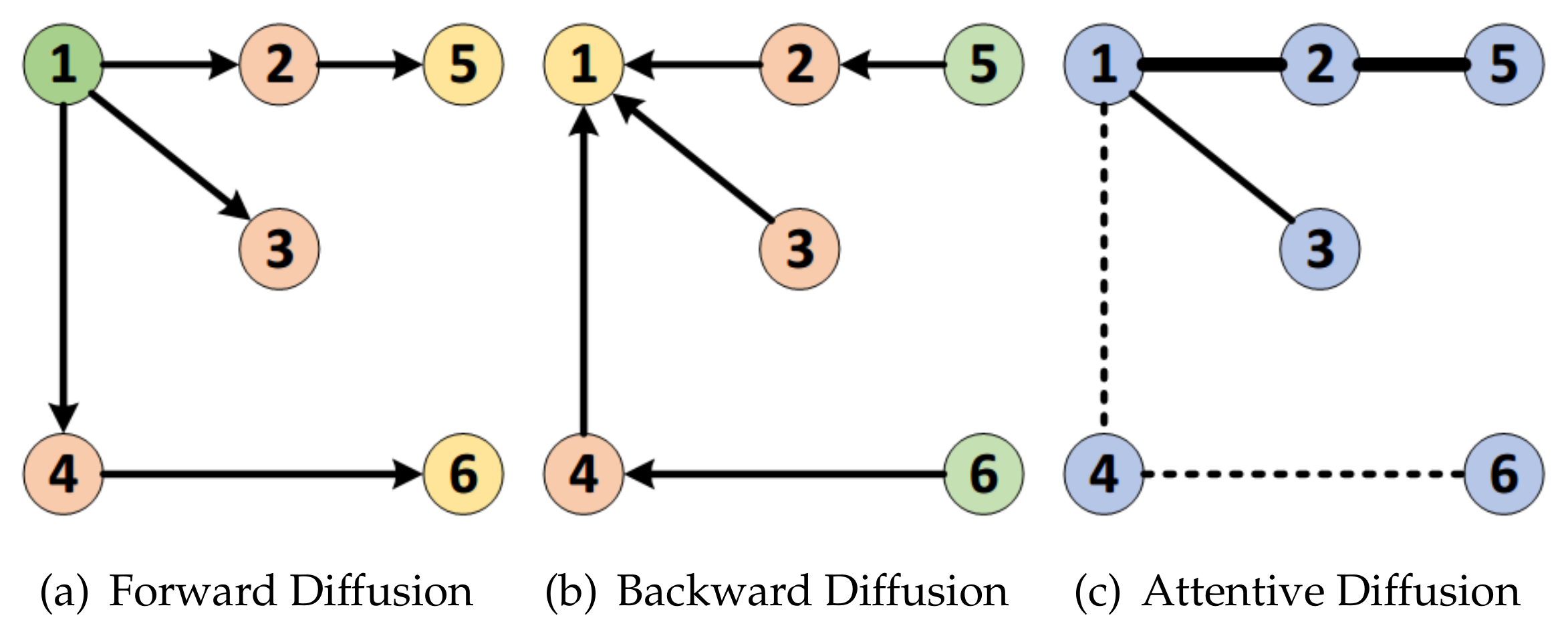
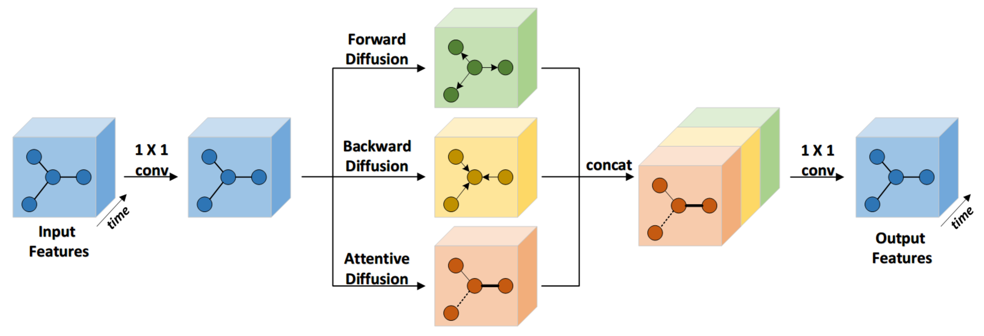
• We propose attentive diffusion convolution to uncover unseen spatial dependencies from traffic graph signals automatically and further present the multi-diffusion convolution block to harvest spatial features in various manners. Extensive experiments demonstrate the ability of our MDC to improve the results when the graph structure is false or unknown.
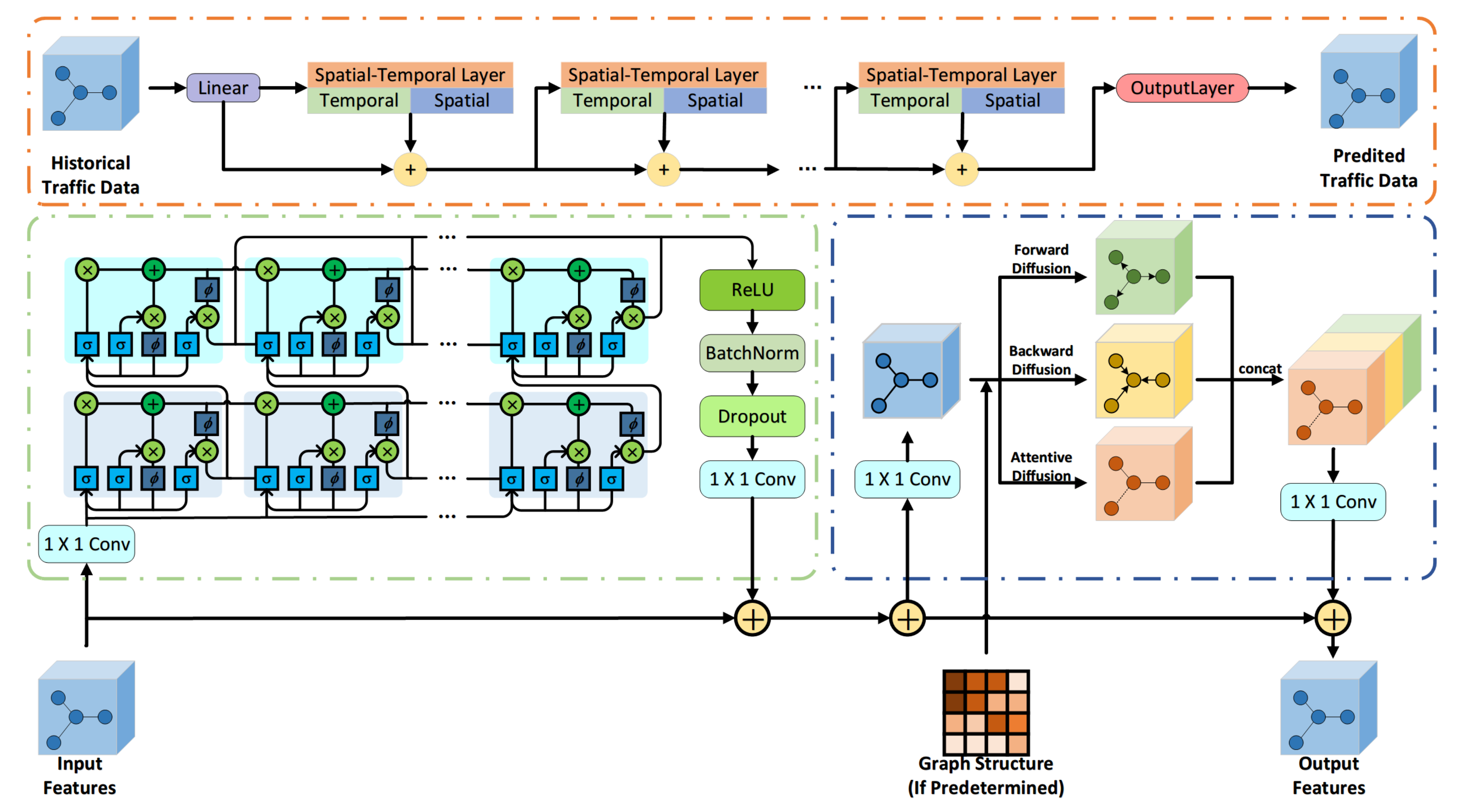
• We construct a novel deep learning hybrid network, the ST-TrafficNet, for spatial-temporal traffic forecasting. The holistic ST-TrafficNet is effective and efficient to capture spatial-temporal features with cascading spatial-temporal layers by adopting residual connections. The core idea of the spatial-temporal layer is to enable our proposed MDC block to tackle spatial dependencies of traffic graph signals with high-dimension temporal features extracted by stacked LSTM block.
• We evaluate ST-TrafficNet on two benchmark datasets and compare it with various baseline methods for traffic forecasting. The experiments show that our proposed method achieves state-of-the-art results in terms of three widely used criteria.

2. Related Works

Traffic flow forecasting is a classical problem that has been being searched for decades [11]. Early traffic forecasting studies mainly employ model-driven approaches such as Autoregressive Integrated Moving Average (ARIMA) [12] and Kalman Filter (KF) family [13,14,15,16]. Although the data-driven methods have been adopted in research and real world applications wildly [17,18], these methods fail to deal with complex non-linear traffic node signals due to the stationary assumption of time-series, which only satisfied under limited conditions [6]. The data-driven methods, however, employ machine learning approaches to discover the traffic patterns in the historic traffic data automatically. With the use of machine learning algorithms such as Support Vector Regression (SVR) [19,20], Extreme Learning Machine (ELM) [21], k-Nearest Neighbors algorithm (kNN) [22,23], the early data-driven method is capable to handle the intricate traffic data in high-dimensional Euclidean space considering the non-linearity of data; hence, it achieve remarkable results in traffic forecasting.

Inspired by the great advances of deep learning, recent researches have further boosted the performance of data-driven methods by adopting various sequence-to-sequence deep learning neural networks such as Deep Belief Network (DBN) [24] and Stacked Autoencoder (SAE) [25,26]. Especially, the Recurrent Neural Network (RNN) based data-driven methods are proved to be practical to harvest temporal dependencies of traffic node signals [27,28,29]. However, the spatial correlations are often neglected or barely leveraged with RNN-based methods, and thus they are inefficient in processing the spatial-temporal dependencies of traffic graph signals.

To fully exploit the unique spatial-temporal patterns of traffic network data, researches further integrate Convolutional Neural Network (CNN) or Graph Convolutional Network (GCN) into RNN. Zhang et al. modeled the spatial dependencies as a heatmap image and used a branch of CNN units to extract different spatial properties of crowd traffic [5]. Yao et al. proposed a gated CNN mechanism to capture the potential spatial features and combined them with temporal features that captured by Long Short-Term Memory (LSTM) to tackle the spatial-temporal traffic forecasting problem [8]. However, the applications of CNN are limited on grid structures, while the traffic network has a topology nature as a graph. Compare to CNN methods, GCN methods are more capable to deal with the traffic network graph structure, since the convolution process is done node by node on the graph [30]. Seo et al. proposed Graph Convolutional Recurrent Network (GCRN) to generalize RNN to traffic graph signals structured by an arbitrary graph with GCN [7]. Li et al. proposed Diffusion Convolutional Recurrent Neural Network (DCRNN), which introduced a diffusion convolution operator into Gated Recurrent Units (GRU) [31]; hence, it can capture spatial-temporal dependencies with a recurrent random walks process on traffic network data [6]. Most recently, the hybrid GCN–RNN models achieve state-of-the-art performance of traffic forecasting [32]. These methods require predefined graph structures to function well, which are highly related on the domain knowledge of the traffic engineers. Although the technical conditions of the road pavements are the same, subjected to the social circumstance, such the economics and the demography, the traffic flow pattern may be totally different. Furthermore, the methods suffer from the ineffectiveness to learn high-dimensional temporal features of intricate traffic signals. In this paper, we propose a spatial-temporal deep learning network to address these two shortcomings.

The rest of this paper is organized as follows. Section 3 is the preliminary knowledge of the traffic forecasting, graph diffusion convolution, and graph attention mechanism. Section 4 presents the proposed ST-TrafficNet in detail. Section 5 applies a series of experiments on two benchmark datasets to verify the performance of the proposed method. Section 6 concludes the proposed work and provides some future research directions.

3. Preliminary

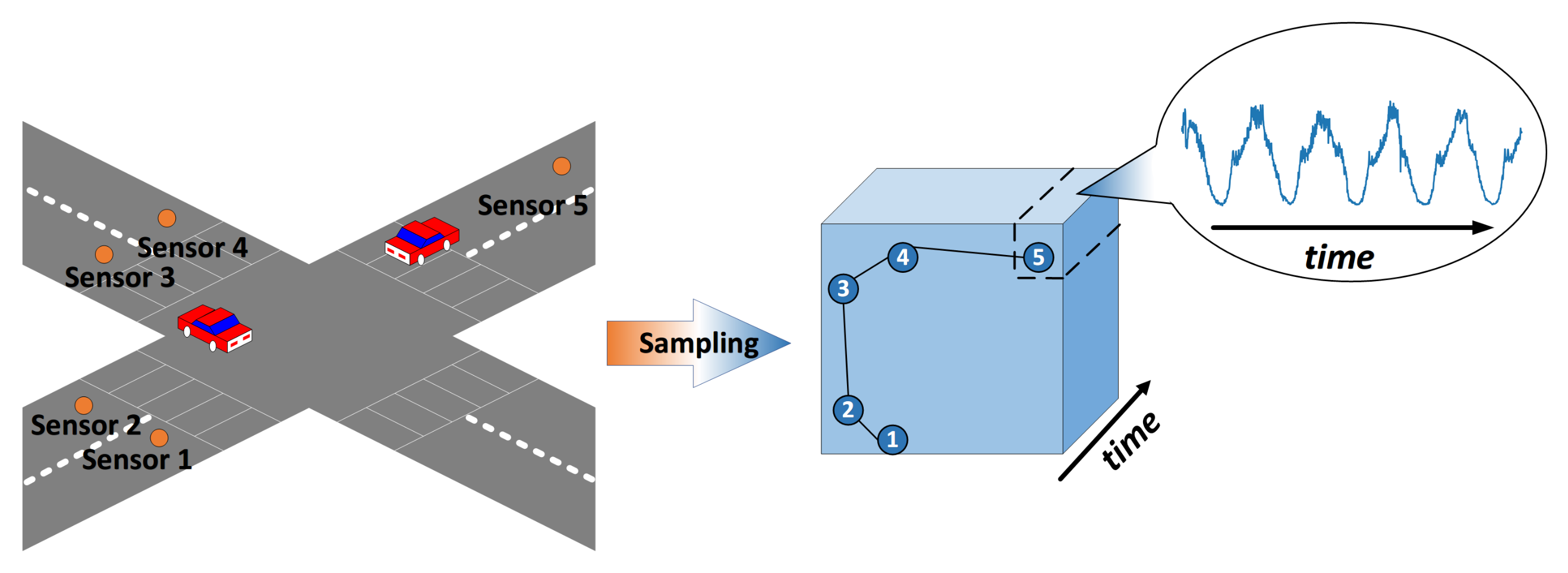
3.1. Traffic Forecasting Modeling

Traffic forecasting is a prediction task to forecast future traffic conditions (e.g., traffic flow, speed) given historical traffic network graph signal observations from a set of sensors in the traffic network. A traffic network can be represented as a graph $\mathcal{G}=(\mathcal{V},\mathcal{E})$, where $\mathcal{V}$ is the set of nodes and $v\in \mathcal{V}$ denotes a sensor on the traffic network, $\mathcal{E}$ is the set of edges and $e\in \mathcal{E}$ denotes a road segment. At time-step t, the graph signal can be observed as $\mathit{X}\in {\mathbb{R}}^{N\times D}$, where N is the number of the nodes and D is the number of traffic parameters (e.g., velocity, volume). Given a graph $\mathcal{G}$ and the past M step graph signals, the problem aims to learn a function $f(·)$ to forecast the following H step graph signals:

$$[{\mathit{X}}^{(t-M+1)}:{\mathit{X}}^{\left(t\right)};\mathcal{G}]\stackrel{f(·)}{⟶}[{\mathit{X}}^{(t+1)},\cdots ,{\mathit{X}}^{(t+H)}].$$

(1)

when the graph structure is unavailable, a learned function $h(·)$ should map the historical node signals to the future without graph structure information input:

$$[{\mathit{X}}^{(t-M+1)}:{\mathit{X}}^{\left(t\right)}]\stackrel{h(·)}{⟶}[{\mathit{X}}^{(t+1)},\cdots ,{\mathit{X}}^{(t+H)}].$$

(2)

3.2. Graph Diffusion Convolution

Graph diffusion convolution was proposed by Li et al. and proved to be effective to capture spatial dependencies of graph signals [6]. A diffusion process on Graph $\mathcal{G}$ is defined as a random walk process with restart probability $\alpha$ and transition matrix $D_O^{-1}W$, where $D_O=diag\left(Wu\right)$ denotes the out-degree diagonal matrix and $u\in {\mathbb{R}}^N$ is a vector of all ones. As a typical Markov process, the diffusion process is able to converge to a stationary distribution $\mathcal{S}\in {\mathbb{R}}^{N\times N}$ after many time-steps. The ith row of $\mathcal{S}$ represents the spatial dependencies between the node $v_i\in \mathcal{V}$ and the others; hence, it captures the latent spatial feature of $\mathcal{G}$. A closed-form of the diffusion process is proposed to calculate it as a weighted combination of infinite random walks on the graph [33]:

$$\mathcal{S}=\sum _{k=0}^{\infty }\alpha {(1-\alpha )}^k{\left({\mathit{D}}_O^{-1}\mathit{W}\right)}^k,$$

(3)

where k is the random walk step. To apply diffusion progress on the task of capturing spatial relationship in graph signals $X\in {\mathbb{R}}^{N\times D}$ with function f, Li et al. propose diffusion convolution [6], which considers finite time-steps K and assign trainable weight parameters:

$$f_{\mathcal{P}}(X,\mathcal{G})=\sum _{k=0}^{K-1}{\mathcal{P}}_k{\left({\mathit{D}}_O^{-1}\mathit{W}\right)}^k\mathit{X},$$

(4)

where $\mathcal{P}\in {\mathcal{R}}^K$ denotes the trainable parameters for each step. In the case of a directed graph, diffusion in one direction only is not enough to discover the latent graph information. Therefore, the diffusion convolution has two directions, forward and backward, and the bidirectional diffusion convolution can be defined as:

$$f_{\mathcal{P}}(X,\mathcal{G})=\sum _{k=0}^{K-1}{\mathcal{P}}_{k,f}{\left({\mathit{D}}_O^{-1}\mathit{W}\right)}^k\mathit{X}+{\mathcal{P}}_{k,b}{\left({\mathit{D}}_I^{-1}{\mathit{W}}^{\top }\right)}^k\mathit{X},$$

(5)

where ${\mathit{D}}_I^{-1}{\mathit{W}}^{\top }$ is the transition matrix of backward diffusion and ${\mathcal{P}}_f$, ${\mathcal{P}}_b$ represent the trainable parameters for each step of forward and backward diffusion convolution, respectively. By employing bidirectional diffusion convolution, spatial dependencies can be captured more flexibly on various kinds of graphs.

3.3. Graph Attention Mechanism

Attention mechanisms, especially graph attention mechanisms [34], have been widely applied to various graph modeling domains due to their flexibility and high efficiency in learning spatial dependencies [35,36,37]. The graph attention mechanism is an enhanced self-attention strategy [35] that is applied on a Graph Convolution Network [30,38]. The most significant improvement of GAM is the way it accumulates the features of adjacent nodes during convolution. We formulate a graph convolution process at the graph level includes the standardized sum of the features of neighbor nodes as:

$${\mathcal{H}}^{l+1}=\sigma \left(\mathcal{C}{\varphi }^l{\mathcal{H}}^l\right),$$

(6)

where $\sigma$ denotes a non-linear activation function (e.g., ReLU, Sigmoid), $\mathcal{C}$ is the matrix of standardized constant induced by graph structure, ${\varphi }^l$ is the trainable weight matrix for node feature transformation in current layer, and ${\mathcal{H}}^l$, ${\mathcal{H}}^{l+1}$ represent the nodes features of the current and next layer, respectively.

GCN requires prior graph structure knowledge to calculate the relationship among nodes, which often is missed in various tasks. Instead of using a standardized constant matrix, GAM uses the attention coefficients matrix to discover graph structure automatically.

Given the layer input ${\mathcal{H}}^l=\left\{h_1^l,h_2^l,\dots h_N^l\right\},h_i^l\in {\mathbb{R}}^D$, where N is the number of nodes and D denotes the number of features of each node. To transform the input into higher dimension features, a shared weight matrix $\varphi \in {\mathcal{R}}^{D\times D^{{}^{\prime }}}$ is adopted:

$$\mathcal{E}=a(\varphi {\mathcal{H}}^l,\varphi {\left({\mathcal{H}}^l\right)}^{-1}),$$

(7)

where a denotes the self-attention mechanism and $\mathcal{E}$ is the original attention coefficients matrix. The normalized attention coefficients matrix is then calculated:

$$A=softmax\left(leakyReLU\right(\mathcal{E}\left)\right).$$

(8)

A leakyReLU activation function is used to eliminate weak attention, then the softmax function is applied to normalize the attention coefficients matrix into an easily comparable form.

Finally, the normalize attention coefficients matrix A is used to update GCN by replacing the standardized constant matrix $\mathcal{C}$ [38]:

$${\mathcal{H}}^{l+1}=\sigma \left(A{\varphi }^l{\mathcal{H}}^l\right).$$

(9)

4. Methodology

4.1. Spatial Aware Multi-Diffusion Convolution Block

In our work, we propose multi-diffusion convolution, in which we introduce GAM into diffusion convolution and present attentive diffusion convolution. Compared to the bidirectional diffusion convolution, ADC does not require any predetermined graph structure knowledge but learns it by self-attention, thus is able to capture hidden spatial dependencies automatically. We first initialize two node embedding vectors $N_h,N_t\in {\mathcal{R}}_N$, named head node and tail node, respectively. Then we construct a trainable transition matrix by multiplying $N_h$ and $N_t$, and induce an attentive transition matrix $A_{att}$ with GAM:

$$A_{att}=softmax\left(leakyReLU\left(N_h{N}_t^T\right)\right).$$

(10)

The transition matrix $N_h{N}_t^T$ implies the potential spatial dependencies from each $N_h$ to each $N_t^T$. After connecting nodes, a leakyReLU activation function is used to eliminate weak connection, then a softmax function is adopted to normalize the transition matrix and make sure that it converges into a stable status after the training process. In the case of the predetermined graph, both the bidirectional diffusion and ADC are available in MDC:

$$\begin{array}{cc}\hfill f_{\mathcal{P}}(X,\mathcal{G})=\sum _{k=0}^{K-1}& {\mathcal{P}}_{k,f}{\left({\mathit{D}}_O^{-1}\mathit{W}\right)}^k\mathit{X}+{\mathcal{P}}_{k,b}{\left({\mathit{D}}_I^{-1}{\mathit{W}}^{\top }\right)}^k\mathit{X}\hfill \\ \hfill & +{\mathcal{P}}_{k,a}{A}_{att}^k\mathit{X}\hfill \end{array}.$$

(11)

The three kinds of diffusion convolution in MDC are shown in Figure 2. In the forward diffusion convolution process, it diffuses from the current node to each kth in the nodes chain and every ith nodes share the same weight while $i\le k$. In the backward diffusion convolution process, it diffuses from each node that can reach the current node with k time-steps. In the ADC process, however, it does not share any weight. The weight between every two nodes is calculated based on GAM and used only in one nodes chain. Since the weight is trainable, ADC is able to correct false or missing connections. The MDC combines different diffusion convolution together to discover the spatial dependencies with various kinds of graph structure flexibly and accurately. In the case of missing graph structure, we propose using ADC independently to discover the potential spatial relationship:

$$h_{\mathcal{P}}\left(X\right)={\mathcal{P}}_{k,a}{A}_{att}^k\mathit{X}.$$

(12)

Next, we further propose an MDC block that can be trained end-to-end through stochastic gradient descent, as illustrated in Figure 3. First, we use a 1 × 1 convolution to simulate a hidden-to-hidden data translation and increase the feature dimensions of the input traffic graph signal features in order to enhance learning ability. Then we perform MDC with three channels, which are forward channel, backward channel, and attentive, respectively. Each channel implements diffusion convolution on high-dimension traffic graph signal features in parallel. Lastly, we concatenate the results and use a 1 × 1 convolution to simulate a hidden-to-output translation and produce the output MDC features.

4.2. Temporal Aware Stacked LSTM Block

We adopt the Long Short-Term Memory recurrent network [39] to capture the temporal trend and seasonality of node signals. As a practical variant of RNN, LSTM allows controlling the flow of information by employing the gated units and cell states; hence, it is able to solve the vanishing gradient problem efficiently. A typical LSTM network consists of LSTM cells, which contain input gate i, forget gate f, and output gate o. With the gated mechanism, LSTM cells are capable to add or remove information from cell state c and generate layer output h. Given the current node signal $x_t$, the LSTM can be represented as four iterating modules:

$$\left(\begin{array}{c}{i}_t\hfill \\ f_t\hfill \\ o_t\hfill \\ g_t\hfill \end{array}\right)=\left(\begin{array}{c}\sigma \\ \sigma \\ \sigma \\ tanh\end{array}\right)\mathit{W}\left(\begin{array}{c}{h}_{t-1}\\ x_t\end{array}\right),$$

(13)

where $\sigma$ denotes the element-wise sigmoid function and $tanh$ is the element-wise hyperbolic tangent function. $\mathit{W}$ is the weighted transition matrix of the iteration process. After an iteration, the cell state $c_t$ is updated and layer output $h_t$ is produced:

$$\begin{array}{cc}\hfill c_t& =f_t\odot c_{t-1}+i_t\odot g_t\hfill \\ \hfill h_t& =o_t\odot tanh\left(c_t\right)\hfill \end{array},$$

(14)

where ⊙ denotes element-wise product. Furthermore, we present a stacked LSTM block, as illustrated in Figure 4 (left-bottom), to capture high-dimension temporal features to discover the temporal dependencies of the traffic graph signals. We first resize the input graph signal’s feature into individual node signals employing 1 × 1 convolution. We then stack multiple LSTM layers to improve the performance of LSTM capturing temporal features with multi scales of time (e.g., day, week, month) [40]. The second LSTM layer receives the hidden cell states of the previous layer as the node signals input; thus, it can harvest relatively high-dimension features based on the low-dimension features input. A ReLu function follows the staked LSTMs and a batchnormalizer [41] regularizes the features to eliminate weak temporal multi-scale features. Instead of element dropout, we apply temporal dropout strategy [42] to zero the entire temporal features with a dropout rate $d_{\theta }$. Finally, we adopt another 1 × 1 convolution to resize the node signals into graph signals for the following spatial-aware block.

4.3. Framework of Spatial-temporal Deep Leaning Network

We present an end-to-end deep learning framework to tackle the spatial-temporal traffic forecasting problem in Figure 4 (top). The proposed framework consists of a linear function to rescale the input data, stacked spatial-temporal layers with residual connection, and an output layer. A spatial-temporal layer is constructed by a LSTM-based block and MDC block, shown in Figure 4 (bottom left) and Figure 4 (bottom right), respectively. The residual connection is adopted in the workflow of the LSTM-based block and MDC block to stabilize the learning process when it goes deep [43] and harvest multi-scale spatial-temporal features. At the first few layers, the stacked LSTM-based block captures relatively low-dimension temporal features and has a limited descriptive ability for temporal traffic data; hence, the MDC block can only learn the spatial features of few temporal traffic patterns. As the network goes deeper, high-dimension temporal features are harvest by stacked LSTM, and the MDC block is able to discover potential spatial dependencies of multi-scale temporal traffic patterns.

It then goes on an output layer equipped with the attention mechanism [35] forecasts the future traffic graph signal:

$$\widehat{X}=\sum _{t=1}^{T-1}\psi \left({\mathcal{F}}_T,{\mathcal{F}}_t\right)·X_{t+1}{\mathit{W}}_o,$$

(15)

where $\widehat{X}$ is the forecast result, ${\mathcal{F}}_t\in {\mathcal{R}}^{N\times D}$ denotes the spatial-temporal features at time t, and $W_o$ represents a trainable weight matrix. Especially, the Frobenius inner product $\psi (·,·)$ of ${\mathcal{F}}_T$ and ${\mathcal{F}}_t$ maps the current features to historical feature according to the similarity. Lastly, we use the MSE loss function to train the end-to-end model with the ground truth traffic graph signals $\tilde{X}$:

$$\mathcal{L}\left(\theta \right)=\parallel \tilde{X}-\widehat{X}{\parallel }_2^2={∥X-f_{\theta }(X,\mathcal{G})∥}_2^2.$$

(16)

5. Experiments and Discussion

5.1. Data Preparation

We employ two real-world large-scale benchmark datasets, which are widely used [6,44,45], to verify ST-TrafficNet. These two datasets not only include rush hours and non-rush hours, but also weekdays and weekends. The first dataset is from the highway of Los Angeles County (METR-LA). The traffic data from a road network consist of 207 loop detectors collected from 1 March 2012 to 30 June 2012, see Figure 5 for more details. The second dataset was collected from the largest publicly available database, e.g., Caltrans Performance Measurement System (PeMS). Three hundred and twenty-five loop detectors in the Bay Area (PEMS-BAY) are selected and the data were collected from 1 January 2017 to 31 May 2017, see Figure 6 for more details. The vehicle loop detector is a kind of sensor that detects vehicles passing or arriving at a road segment. It is often installed under the pavement. The wire loops are supplied alternating current at frequencies between 10 kHz to 200 kHz by the electronics unit. In this way, the loop wire behaves as a tuned electrical circuit. When a vehicle passes over the loop or is stopped within the loop, the ferrous body material of the vehicle changes the inductance of the loop wire. This change can be detected to report the occupation of the loop, see [46] for more details.

The original data collected from sensors are sliced with a 5-min time interval window. The traffic flow data aggregated in small time intervals are easily affected by outliers, which will decrease the accuracy of the forecasting models. On the other hand, traffic flow data of too large time intervals provide little information for forecasting [14]. Since we do not intend to forecast the minute to minute fluctuations, the 5-min time interval window is a rational setting. To initialize the graph structure of the traffic network, a Gaussian kernel thresholded algorithm [47] is used to calculate the correlation between every two nodes and construct the adjacency matrix $W=\left\{w_{ij}\right\}$ of the graph by:

$$w_{ij}=\{\begin{array}{cc}exp(-\frac{dist{(v_i,v_j)}^2}{{\sigma }^2}),\hfill & dist\left(v_i,v_j\right)\le \kappa ,\hfill \\ 0,\hfill & \mathrm{otherwise},\hfill \end{array}$$

(17)

where $dist(v_i,v_j)$ denotes the distance of the road segment between $v_i$ and $v_j$. $\sigma$ is the standard deviation of distances and $\kappa$ is the threshold. The dataset is then Z-score normalized and split into training set (70%), validation set (10%), and test set (20%).

5.2. Baseline Methods

We compare ST-TrafficNet with various baseline methods. First, three model-driven methods: Historical Average (HA) [6], Auto-Regressive Integrated Moving Average (ARIMA) [6], and Linear Support Vector Regression (LSVR) [45]. The order of the ARIMA is $ARIMA(3,0,1)$. We employ the statsmodel python package for the implementation. We run the ARIMA on each measurement point. Second, three data-driven methods without using spatial factors are selected: Feed forward Neural Network (FNN) [45], Fully-Connected LSTM (FC-LSTM) [6], and WaveNet [48]. Finally, four state-of-the-art data-driven methods designed for spatial-temporal graph modeling are chosen: Diffusion Convolution Recurrent Neural Network (DCRNN) [6], Spatial-Temporal Graph Convolution Network (STGCN) [49], Spatio-Temporal U-Network (ST-UNet) [45], and Graph WaveNet (GWaveNet) [44].

5.3. Experimental Setup and Evaluation Criteria

All the experiments were conducted under a computer environment with dual NVIDIA GeForce RTX 2080ti GPU and an Intel(R)Core(TM)i9-7900X CPU @3.30GHz. Eight spatial-temporal layers were cascaded together to harvest spatial-temporal features. The random walk step K in the MDC process was set to 2, and the time-step of stacked LSTM was set to 32 and 128 for two LSTM layers, respectively. The dropout rate of stacked LSTM was 0.2. ST-TrafficNet is trained based on the Adam optimizer [50] for 200 epochs with early stopping. The initial learning rate was 0.001 with a weight decay of 3 × 10⁻⁴; the batch size was set to 128.

Three criteria are employed to quantitatively evaluate the traffic forecasting performance: Mean Absolute Error (MAE), Root Mean Square Error (RMSE), and Mean Absolute Percentage Error (MAPE), defined as follows:

$$\mathrm{MAE}=\frac{1}{T}\sum _{i=1}^T\left|{\mathit{X}}_i-{\widehat{\mathit{X}}}_i\right|,$$

(18)

$$RMSE=\sqrt{\frac{1}{T}\sum _{t=1}^T{({\widehat{\mathit{X}}}_t-{\mathit{X}}_t)}^2},$$

(19)

$$MAPE=\frac{1}{T}\sum _{t=1}^T\left|\frac{{\widehat{\mathit{X}}}_t-{\mathit{X}}_t}{{\mathit{X}}_t}\right|,$$

(20)

where ${\mathit{X}}_t$ is the observed graph signal at time-step t, and ${\widehat{\mathit{X}}}_t$ is the predicted graph signal.

5.4. Performance Comparison

Table 1. Performance comparisons with baseline methods on METR-LA dataset. Our spatial-temporal deep learning network (ST-TrafficNet) achieves the best results.

METR-LA Dataset		15 min			30 min			60 min
	MAE	RMSE	MAPE	MAE	RMSE	MAPE	MAE	RMSE	MAPE
	(Vehs)	(Vehs)	(%)	(Vehs)	(Vehs)	(%)	(Vehs)	(Vehs)	(%)
HA	4.16	7.80	13.00	4.16	7.80	13.00	4.16	7.80	13.00
ARIMA	3.99	8.21	9.60	5.15	10.45	12.70	6.90	13.23	17.40
LSVR	2.97	5.89	7.68	3.64	7.35	9.90	4.67	9.13	13.63
FNN	3.99	7.94	9.91	4.23	8.17	12.92	4.49	8.69	14.01
FC-LSTM	3.44	6.30	9.60	3.77	7.23	10.90	4.37	8.69	13.20
WaveNet	2.99	5.89	8.04	3.59	7.28	10.25	4.45	8.93	13.62
STGCN	2.88	5.74	7.62	3.47	7.24	9.57	4.59	9.40	12.70
DCRNN	2.77	5.38	7.30	3.15	6.45	8.80	3.60	7.60	10.50
ST-UNet	2.83	5.17	7.03	3.22	6.36	8.63	3.65	7.40	10.00
GWaveNet	2.70	5.15	6.92	3.09	6.22	8.37	3.55	7.37	10.01
ST-TrafficNet	2.56	5.06	6.82	2.89	6.17	8.35	3.46	7.29	9.89

and

Table 2. Performance comparisons with baseline methods on PEMS-BAY dataset. Our ST-TrafficNet achieves the best results.

PEMS-BAY Dataset		15 min			30 min			60 min
	MAE	RMSE	MAPE	MAE	RMSE	MAPE	MAE	RMSE	MAPE
	(Vehs)	(Vehs)	(%)	(Vehs)	(Vehs)	(%)	(Vehs)	(Vehs)	(%)
HA	2.88	5.59	6.80	2.88	5.59	6.80	2.88	5.59	6.80
ARIMA	1.62	3.30	3.50	2.33	4.76	5.40	3.38	6.50	8.30
LSVR	1.42	3.45	3.31	2.13	4.37	5.28	2.34	4.28	5.55
FNN	1.59	3.42	3.53	2.11	4.42	5.16	3.18	6.24	8.12
FC-LSTM	2.05	4.19	4.80	2.20	4.55	5.20	2.37	4.96	5.70
WaveNet	1.39	3.01	2.91	1.83	4.21	4.16	2.35	5.43	5.87
STGCN	1.36	2.96	2.90	1.81	4.27	4.17	2.49	5.69	5.79
DCRNN	1.38	2.95	2.90	1.74	3.97	3.90	2.37	4.94	5.30
ST-UNet	1.38	2.83	2.79	1.72	3.82	3.75	1.97	4.63	4.83
GWaveNet	1.31	2.74	2.73	1.63	3.70	3.67	1.98	4.65	4.92%
ST-TrafficNet	1.26	2.72	2.68	1.58	3.57	3.59	1.93	4.61	4.88

report the comparison of ST-TrafficNet and 10 baseline methods on two benchmark datasets for 3, 6, and 12 time-steps, respectively. The experiment result shows that ST-TrafficNet surpasses the baseline methods on both benchmark datasets for different scales of time.

We can observe that data-driven methods achieve a greater performance than the model-driven methods (HA, ARIMA, and LSVR), demonstrating the ability of data-driven methods to learn more comprehensive features by deploying neural network architecture. Compared to the temporal data-driven methods (FNN, F-CLSTM, and WaveNet), the spatial-temporal data-driven methods are capable to use the graph structure of traffic network to help forecasting graph signal on each node, therefore outperforming all the temporal data-driven methods. ST-TrafficNet is superior to the state-of-the-art spatial-temporal data-driven methods. Regarding the DCRNN method, the mean MAE on two datasets of ST-TrafficNet outperforms DCRNN by 8.15% (15 min), 8.65% (30 min), and 9.4% (60 min). DCRNN is comparable to ST-TrafficNet in terms of neural network structure since it combines diffusion convolution with Recurrent Neural Network together to forecasting spatial-temporal traffic graph signal. In that respect, ST-TrafficNet is more capable to capture complicated and subtle spatial-temporal patterns for three reasons: (1) The attentive diffusion convolution in the MDC block provides a more comprehensive understanding of the spatial dependencies than the predefined graph structure based on human knowledge, which is adopted in DCRNN. Consequently, ST-TrafficNet outperforms DCRNN for all three time scales. (2) Compared to the simple Recurrent Neural Network, temporal-aware LSTM-based blocks in each spatial-temporal layer can tackle high-dimension temporal features and describe the temporal node signals; hence, the ST-TrafficNet is able to deal with short-term and long-term temporal dependencies, respectively. Therefore, the MAE drop at 60 min time-step is greater than 30 min and 15 min. (3) The stacked neural network is always shallow on account of the gradient explosion issue. However, ST-TrafficNet stack spatial-temporal layers with residual connections, and stabilize the performance of each layer.

We further provide a visual comparison between DCRNN and ST-TrafficNet in Figure 7, which shows the forecasting result and ground truth traffic signals of a node in a day. The node locates in a dense area of PeMS-BAY; hence, the spatial dependencies are significant to improve the forecasting performance. As the comparison shows, the curve of ST-TrafficNet is closer to the ground truth and the curve of DCRNN is smoother while the ground truth changes rapidly. At the peak hour of the day, an impulsive disturbance is created by unexpected factors. The DCRNN is affected and the prediction deviates far from ground truth, but the stable performance of ST-TrafficNet remains due to the benefit of using the self-learned spatial features.

5.5. Efficacy of Multi-Diffusion Convolution Block

We further conduct experiments on ST-TrafficNet with four different MDC block configurations to verify the efficacy of the proposed MDC block. Firstly, we take off the MDC block from ST-TrafficNet to verify the network with only temporal features as a benchmark. Secondly, an MDC block consists of only attentive channel is used to verify the ability to learn potential spatial features without any prior graph structure knowledge. We then configure the MDC block with the forward and backward channels, which are flexible to capture spatial dependencies from the predetermined graph. The last ST-TrafficNet adopted a three-channel NDC block, which makes it to be the proposed ST-TrafficNet. We compare the four different ST-TrafficNets on both METR-LA and PeMS-BAY datasets with 15 min, 30 min, and 60 min time-steps. The experiment results are shown in

Table 3. The case study results of ST-TrafficNets with different MDC block configurations. All the MDC models surpass the temporal-only model largely. The attentive-only model is just little poorer than the forward-backward model. The forward-backward-attentive model achieves the best result.

Data-Set	Model		15 min			30 min			60 min
		MAE	RMSE	MAPE	MAE	RMSE	MAPE	MAE	RMSE	MAPE
		(Vehs)	(Vehs)	(%)	(Vehs)	(Vehs)	(%)	(Vehs)	(Vehs)	(%)
	T(Temporal only)	3.36	6.27	9.61	3.75	7.21	10.92	4.34	8.65	13.21
METR-	$C_a$(Attentive only)	2.81	5.32	7.36	3.12	6.46	8.56	3.69	7.48	10.42
LA	$C_f-C_b$(without Attentive)	2.68	5.19	7.01	2.95	6.31	8.48	3.57	7.36	10.01
	$C_f-C_b-C_a$(proposed model)	2.56	5.06	6.82	2.89	6.17	8.35	3.46	7.29	9.89
	T(Temporal only)	2.02	4.14	4.78	2.20	4.54	5.19	2.34	4.94	5.70
PEMS-	$C_a$(Attentive only)	1.41	2.86	2.79	1.74	3.80	3.91	2.13	4.78	5.17
BAY	$C_f-C_b$(without Attentive)	1.33	2.74	2.75	1.66	3.68	3.73	2.01	4.69	5.00
	$C_f-C_b-C_a$(proposed model)	1.26	2.72	2.68	1.58	3.57	3.59	1.93	4.61	4.88

. The performance of three ST-TrafficNets using diffusion convolution surpasses the temporal-only ST-TrafficNet largely, indicating the significance of diffusion convolution capturing spatial features while tackling spatial-temporal traffic forecasting. By employing the attentive diffusion channel only MDC block, attentive-only ST-TrafficNet performs just a little poorer than forward-backward ST-TrafficNet, showing the functionality of attentive diffusion convolution while no graph structure information is available. The proposed ST-TrafficNet outperforms the forward-backward ST-TrafficNet with the attentive channel, indicating that even if the prior graph structure knowledge is given, the MDC block can still discover useful spatial features.

The computational times of ARIMA and ST-TrafficNet on dataset METR-LA are listed in

Table 4. The computational time of Autoregressive Integrated Moving Average (ARIMA) and ST-TrafficNet on dataset METR-LA.

Model	Computational Time
	Train (Seconds/Epoch)	Predict (Seconds)
ARIMA	-	0.94
ST-TrafficNet	83.74	3.52

. The ARIMA(p, q, d) needs not really to be trained. It needs to properly select the order of Auto Regressive (AR) term p, the order of the moving average (MA) term q, and the number of differencing d. The order of the AR term is the number of lags to be used as predictors in the linear regression model. Traffic engineers determined the order of the AR term to guarantee the predictors are not correlated and are independent of each other according the traffic situation of the road segment. The MA term refers to the number of lagged forecast errors that go into the ARIMA. The number of differencing depends on the complexity of the traffic flow, more than one differencing may be needed. More details of ARMIA could be found in [51]. Our model takes 83.74 seconds for every epoch. It converges after 50 to 60 epochs. Different from the parametric models, training a deep learning network requires tedious time to iteratively optimize the parameters in each layer, but the prediction needs only one forward propagation. Thus, the prediction stage is much faster than its training stage. Fortunately, the deep learning network only needs to be trained once, and can be conducted off-line. Moreover, both stages can accelerate by the GPUs. Our model takes 274% more computational time than the ARIMA, but achieves over 43.19% more accuracy of MAE (average by 15/30/60 min) than the ARIMA.

5.6. Influence of Missing and Incorrect Graph Structure Knowledge

To many data-driven spatial-temporal methods, good quality of traffic graph signals and graph structure is significant. However, traffic network graph structure from human knowledge or simple distance algorithm could have false connections (e.g., two close nodes planted on opposite direction carriageways) or missing connections (e.g., two distant nodes planted on the same traffic stream). Therefore, we conduct experiments to test the performance of ST-TrafficNet with or without attentive diffusion convolution on missing and incorrect graph structure. We first sample the noise from Gaussian distributions with a variance which is 5% or 10% of the mean values of graph structure data, and the test data are generated by adding up the noise and original graph structure data. Then another set of graph structure data is zero with the rate 50% or 100% to produce the missing dataset. Both the experiment employ PeMS-BAY as the original dataset with 15 min time-steps.

The MAE scores of two experiments are presented in

Table 5. The Mean Absolute Error (MAE) score of ST-TrafficNet with or without attentive diffusion convolution on missing and incorrect graph structure. Under the condition of incorrect graph structure with 5% noise, the proposed model remains nearly the same while the non-attentive model degenerates by 3%. Under the condition of unavailable predetermined graph structure (i.e., missing rate 100%), the non-attentive model dropped by 51.9% and the proposed model only degenerates by 11.9%.

Disturbance		ST-TrafficNet	ST-TrafficNet
		(${\mathit{C}}_{\mathit{f}}\mathbf{-}{\mathit{C}}_{\mathit{b}}$)	(${\mathit{C}}_{\mathit{f}}\mathbf{-}{\mathit{C}}_{\mathit{b}}\mathbf{-}{\mathit{C}}_{\mathit{a}}$)
	original	1.33	1.26
noise	5%	1.37	1.26
	10%	1.44	1.29
	original	1.33	1.26
missing	50%	1.57	1.29
	100%	2.02	1.41

. When the predetermined graph structure data are disturbed by 5% Gaussian noise, the MAE score of non-attentive ST-TrafficNet convolution degenerates by 3% while the proposed ST-TrafficNet almost does not change, and the performance of non-attentive ST-TrafficNet degenerate more rapidly while the ST-TrafficNet decay with a relatively slower rate under a 10% Gaussian noise condition due to the ability to correct the false connection. As for the missing data, the non-attentive ST-TrafficNet turns into a temporal-only ST-TrafficNet when the missing rate goes to 100%, but ST-TrafficNet can use attentive diffusion convolution to learn latent spatial dependencies from graph signals and deliver higher performance. Consequently, the MAE score of non-attentive ST-TrafficNet degenerates by 51.9% and only an 11.9% penalty is developed for ST-TrafficNet.

The traffic flow speed is critically important to discriminate the traffic state. Actually, our method can predict traffic speed if the training data contain traffic speed. Furthermore, our method can be extended to other spatial-temporal applications, such as grid load forecasting.

6. Conclusions

In this paper, we propose a novel spatial-temporal deep learning network for traffic forecasting. The proposed attentive diffusion convolution can automatically capture various spatial dependencies, which are difficult if not impossible to be predefined by traffic engineers. Equipped with our attentive diffusion convolution and cascaded LSTM block, our ST-TrafficNet effectively uncovers the spatial-temporal relations inside the traffic flow data. Sufficient experiments on two public benchmark traffic flow datasets show that the proposed model achieves state-of-the-art performance. The future works will be focused on two aspects. First, we are trying to design new deep learning networks that not only consider the connectivity of the traffic graph, but also the social and economic factors for accurate and timely traffic flow forecasting. Second, we shall apply our methods to more multi-dimensional time series analysis applications, such as grid load forecasting.

References

1. Di Febbraro, A.; Giglio, D.; Sacco, N. A deterministic and stochastic Petri net model for traffic-responsive signaling control in urban areas. IEEE Trans. Intell. Transp. Syst. 2015, 17, 510–524. [Google Scholar] [CrossRef]
2. Boriboonsomsin, K.; Barth, M.J.; Zhu, W.; Vu, A. Eco-routing navigation system based on multisource historical and real-time traffic information. IEEE Trans. Intell. Transp. Syst. 2012, 13, 1694–1704. [Google Scholar] [CrossRef]
3. Veres, M.; Moussa, M. Deep learning for intelligent transportation systems: A survey of emerging trends. IEEE Trans. Intell. Transp. Syst. 2019, 21, 3152–3168. [Google Scholar] [CrossRef]
4. Zambrano-Martinez, J.L.; Calafate, C.T.; Soler, D.; Cano, J.C.; Manzoni, P. Modeling and characterization of traffic flows in urban environments. Sensors 2018, 18, 2020. [Google Scholar] [CrossRef] [Green Version]
5. Zhang, J.; Zheng, Y.; Qi, D. Deep spatio-temporal residual networks for citywide crowd flows prediction. In Proceedings of the Thirty-First AAAI Conference on Artificial Intelligence, San Francisco, CA, USA, 23 June 2017. [Google Scholar]
6. Li, Y.; Yu, R.; Shahabi, C.; Liu, Y. Diffusion Convolutional Recurrent Neural Network: Data-Driven Traffic Forecasting. In Proceedings of the International Conference on Learning Representations, Vancouver, BC, Canada, 30 April–3 May 2018. [Google Scholar]
7. Seo, Y.; Defferrard, M.; Vandergheynst, P.; Bresson, X. Structured sequence modeling with graph convolutional recurrent networks. In Proceedings of the International Conference on Neural Information Processing, Siem Reap, Cambodia, 13–16 December 2018; pp. 362–373. [Google Scholar]
8. Yao, H.; Tang, X.; Wei, H.; Zheng, G.; Li, Z. Revisiting spatial-temporal similarity: A deep learning framework for traffic prediction. In Proceedings of the AAAI Conference on Artificial Intelligence, Honolulu, HI, USA, 27 January–1 February 2019; Volume 33, pp. 5668–5675. [Google Scholar]
9. Zhang, J.; Shi, X.; Xie, J.; Ma, H.; King, I.; Yeung, D.Y. GaAN: Gated Attention Networks for Learning on Large and Spatiotemporal Graphs. arXiv 2018, arXiv:1803.07294. [Google Scholar]
10. Du, X.; Zhang, H.; Van Nguyen, H.; Han, Z. Stacked LSTM deep learning model for traffic prediction in vehicle-to-vehicle communication. In Proceedings of the 2017 IEEE 86th Vehicular Technology Conference (VTC-Fall), Toronto, ON, Canada, 24–27 September 2017; pp. 1–5. [Google Scholar]
11. Zhou, T.; Han, G.; Xu, X.; Han, C.; Huang, Y.; Qin, J. A learning-based multimodel integrated framework for Dynamic traffic flow forecasting. Neural Process. Lett. 2019, 43, 407–430. [Google Scholar] [CrossRef]
12. Li, X.; Pan, G.; Wu, Z.; Qi, G.; Li, S.; Zhang, D.; Zhang, W.; Wang, Z. Prediction of urban human mobility using large-scale taxi traces and its applications. Front. Comput. Sci. 2012, 6, 111–121. [Google Scholar]
13. Guo, J.; Huang, W.; Williams, B.M. Adaptive Kalman filter approach for stochastic short-term traffic flow rate prediction and uncertainty quantification. Transp. Res. Part C Emerg. Technol. 2014, 43, 50–64. [Google Scholar] [CrossRef]
14. Zhou, T.; Jiang, D.; Lin, Z.; Han, G.; Xu, X.; Qin, J. Hybrid dual Kalman filtering model for short-term traffic flow forecasting. IET Intell. Transp. Syst. 2019, 13, 1023–1032. [Google Scholar] [CrossRef]
15. Cai, L.; Zhang, Z.; Yang, J.; Yu, Y.; Zhou, T.; Qin, J. A noise-immune Kalman filter for short-term traffic flow forecasting. Phys. A Stat. Mech. Appl. 2019, 536, 122601. [Google Scholar] [CrossRef]
16. Zhang, S.; Song, Y.; Jiang, D.; Zhou, T.; Qin, J. Noise-identified Kalman filter for short-term traffic flow forecasting. In Proceedings of the 2019 15th International Conference on Mobile Ad-Hoc and Sensor Networks (MSN), Shenzhen, China, 11–13 December 2019; pp. 462–466. [Google Scholar]
17. Moreira-Matias, L.; Gama, J.; Ferreira, M.; Mendes-Moreira, J.; Damas, L. Predicting taxi–passenger demand using streaming data. IEEE Trans. Intell. Transp. Syst. 2013, 14, 1393–1402. [Google Scholar] [CrossRef] [Green Version]
18. Tan, M.C.; Wong, S.C.; Xu, J.M.; Guan, Z.R.; Zhang, P. An aggregation approach to short-term traffic flow prediction. IEEE Trans. Intell. Transp. Syst. 2009, 10, 60–69. [Google Scholar]
19. Castro-Neto, M.; Jeong, Y.S.; Jeong, M.K.; Han, L.D. Online-SVR for short-term traffic flow prediction under typical and atypical traffic conditions. Expert Syst. Appl. 2009, 36, 6164–6173. [Google Scholar] [CrossRef]
20. Cai, L.; Chen, Q.; Cai, W.; Xu, X.; Zhou, T.; Qin, J. SVRGSA: A hybrid learning based model for short-term traffic flow forecasting. IET Intell. Transp. Syst. 2019, 13, 1348–1355. [Google Scholar] [CrossRef]
21. Cai, W.; Yang, J.; Yu, Y.; Song, Y.; Zhou, T.; Qin, J. PSO-ELM: A hybrid learning model for short-term traffic flow forecasting. IEEE Access 2020, 8, 6505–6514. [Google Scholar] [CrossRef]
22. Chang, H.; Lee, Y.; Yoon, B.; Baek, S. Dynamic near-term traffic flow prediction: System-oriented approach based on past experiences. IET Intell. Transp. Syst. 2012, 6, 292–305. [Google Scholar] [CrossRef]
23. Cai, L.; Yu, Y.; Zhang, S.; Song, Y.; Xiong, Z.; Zhou, T. A Sample-rebalanced Outlier-rejected k-nearest Neighbour Regression Model for Short-Term Traffic Flow Forecasting. IEEE Access 2020, 8, 22686–22696. [Google Scholar] [CrossRef]
24. Huang, W.; Song, G.; Hong, H.; Xie, K. Deep architecture for traffic flow prediction: Deep belief networks with multitask learning. IEEE Trans. Intell. Transp. Syst. 2014, 15, 2191–2201. [Google Scholar] [CrossRef]
25. Lv, Y.; Duan, Y.; Kang, W.; Li, Z.; Wang, F.Y. Traffic flow prediction with big data: A deep learning approach. IEEE Trans. Intell. Transp. Syst. 2014, 16, 865–873. [Google Scholar] [CrossRef]
26. Zhou, T.; Han, G.; Xu, X.; Lin, Z.; Han, C.; Huang, Y.; Qin, J. δ-agree AdaBoost stacked autoencoder for short-term traffic flow forecasting. Neurocomputing 2017, 247, 31–38. [Google Scholar] [CrossRef]
27. Mackenzie, J.; Roddick, J.F.; Zito, R. An evaluation of HTM and LSTM for short-term arterial traffic flow prediction. IEEE Trans. Intell. Transp. Syst. 2018, 20, 1847–1857. [Google Scholar] [CrossRef]
28. Yang, B.; Sun, S.; Li, J.; Lin, X.; Tian, Y. Traffic flow prediction using LSTM with feature enhancement. Neurocomputing 2019, 332, 320–327. [Google Scholar] [CrossRef]
29. Cai, L.; Lei, M.; Zhang, S.; Yu, Y.; Zhou, T.; Qin, J. A noise-immune LSTM network for short-term traffic flow forecasting. Chaos Interdiscip. J. Nonlinear Sci. 2020, 30, 023135. [Google Scholar] [CrossRef]
30. Bruna, J.; Zaremba, W.; Szlam, A.; LeCun, Y. Spectral networks and deep locally connected networks on graphs. In Proceedings of the 2nd International Conference on Learning Representations, ICLR 2014, Banff, AB, Canada, 14–16 April 2014. [Google Scholar]
31. Chung, J.; Gulcehre, C.; Cho, K.; Bengio, Y. Empirical evaluation of gated recurrent neural networks on sequence modeling. In Proceedings of the NIPS 2014 Workshop on Deep Learning, Montreal, QB, Canada, 8–13 December 2014. [Google Scholar]
32. Li, G.; Muller, M.; Thabet, A.; Ghanem, B. Deepgcns: Can gcns go as deep as cnns? In Proceedings of the IEEE International Conference on Computer Vision, Seoul, Korea, 27 October–2 November 2019; pp. 9267–9276. [Google Scholar]
33. Teng, S.H. Scalable algorithms for data and network analysis. Found. Trends Theor. Comput. Sci. 2016, 12, 1–274. [Google Scholar] [CrossRef]
34. Veličković, P.; Cucurull, G.; Casanova, A.; Romero, A.; Liò, P.; Bengio, Y. Graph Attention Networks. In Proceedings of the International Conference on Learning Representations, Vancouver, BC, Canada, 30 April–3 May 2018. [Google Scholar]
35. Vaswani, A.; Shazeer, N.; Parmar, N.; Uszkoreit, J.; Jones, L.; Gomez, A.N.; Kaiser, Ł.; Polosukhin, I. Attention is all you need. In Proceedings of the Advances in Neural Information Processing Systems, Long Beach, CA, USA, 4–9 December 2017; pp. 5998–6008. [Google Scholar]
36. Shen, T.; Zhou, T.; Long, G.; Jiang, J.; Pan, S.; Zhang, C. Disan: Directional self-attention network for rnn/cnn-free language understanding. In Proceedings of the Thirty-Second AAAI Conference on Artificial Intelligence, New Orleans, LA, USA, 2–7 February 2018. [Google Scholar]
37. Li, X.; Bai, L.; Ge, Z.; Lin, Z.; Yang, X.; Zhou, T. Early Diagnosis of Neuropsychiatric Systemic Lupus Erythematosus by Deep Learning Enhanced Magnetic Resonance Spectroscopy. J. Med. Imaging Health Inform. In press.
38. Kipf, T.N.; Welling, M. Semi-supervised classification with graph convolutional networks. arXiv 2016, arXiv:1609.02907. [Google Scholar]
39. Hochreiter, S.; Schmidhuber, J. Long short-term memory. Neural Comput. 1997, 9, 1735–1780. [Google Scholar] [CrossRef] [PubMed]
40. Zheng, H.; Lin, F.; Feng, X.; Chen, Y. A Hybrid Deep Learning Model With Attention-Based Conv-LSTM Networks for Short-Term Traffic Flow Prediction. IEEE Trans. Intell. Transp. Syst. 2020. Early Access. [Google Scholar]
41. Ioffe, S.; Szegedy, C. Batch normalization: Accelerating deep network training by reducing internal covariate shift. arXiv 2015, arXiv:1502.03167. [Google Scholar]
42. Srivastava, N.; Hinton, G.; Krizhevsky, A.; Sutskever, I.; Salakhutdinov, R. Dropout: A simple way to prevent neural networks from overfitting. J. Mach. Earn. Res. 2014, 15, 1929–1958. [Google Scholar]
43. He, K.; Zhang, X.; Ren, S.; Sun, J. Deep residual learning for image recognition. In Proceedings of the IEEE Conference on Computer Vision and Pattern Recognition, Las Vegas, NV, USA, 27–30 June 2016; pp. 770–778. [Google Scholar]
44. Wu, Z.; Pan, S.; Long, G.; Jiang, J.; Zhang, C. Graph WaveNet for deep spatial-temporal graph modeling. In Proceedings of the International Joint Conference on Artificial Intelligence 2019, Macao, China, 10–16 August 2019; pp. 1907–1913. [Google Scholar]
45. Yu, B.; Yin, H.; Zhu, Z. ST-UNet: A Spatio-Temporal U-Network for Graph-structured Time Series Modeling. arXiv 2019, arXiv:1903.05631. [Google Scholar]
46. Li, J.; Perrine, K.; Walton, C.M. Identifying Faulty Loop Detectors Through Kinematic Wave Based Traffic State Reconstruction from Transit Probe Data. In Proceedings of the Transportation Research Board 96th Annual Meeting, Washington, DC, USA, 8–12 January 2017; p. 17-04843. [Google Scholar]
47. Shuman, D.I.; Narang, S.K.; Frossard, P.; Ortega, A.; Vandergheynst, P. The emerging field of signal processing on graphs: Extending high-dimensional data analysis to networks and other irregular domains. IEEE Signal Process. Mag. 2013, 30, 83–98. [Google Scholar] [CrossRef] [Green Version]
48. Van den Oord, A.; Dieleman, S.; Zen, H.; Simonyan, K.; Vinyals, O.; Graves, A.; Kalchbrenner, N.; Senior, A.; Kavukcuoglu, K. WaveNet: A Generative Model for Raw Audio. In Proceedings of the 9th ISCA Speech Synthesis Workshop, Sunnyvale, CA, USA, 13–15 September 2016; p. 125. [Google Scholar]
49. Yu, B.; Yin, H.; Zhu, Z. Spatio-Temporal Graph Convolutional Networks: A Deep Learning Framework for Traffic Forecasting. In Proceedings of the International Joint Conference on Artificial Intelligence(IJCAI), Stockholm, Sweden, 13–19 July 2018; pp. 3634–3640. [Google Scholar]
50. Kingma, D.P.; Ba, J. Adam: A method for stochastic optimization. arXiv 2014, arXiv:1412.6980. [Google Scholar]
51. Smith, B.L.; Williams, B.M.; Oswald, R.K. Comparison of parametric and nonparametric models for traffic flow forecasting. Transp. Res. Part C Emerg. Technol. 2002, 10, 303–321. [Google Scholar] [CrossRef]
Figure 1. Complex spatial and temporal dependencies. The traffic network data are sampled as traffic graph signals, which consist of many sets of traffic node signals and the nodes are interrelated as a graph. The temporal dependencies of each set of node signals represent the seasonality and trend. The predetermined graph structure could easily go wrong such as nodes 1 and 2 (false connection), nodes 2 and 5 (missing connection).
Electronics 09 01474 g001
Figure 2. The illustrations of three kinds of diffusion convolution. In (a,b), the direction of the node chain denotes the diffusion direction of current node 1, and the nodes with the same color share the same weight in the diffusion process (e.g., nodes 5,6 share the same weight with time-step k = 2 ). In (c), the edges indicate the relationship between two nodes (e.g., the dotted edge <1,4> indicates a weak connection based on Graph Attention Mechanism (GAM)).
Electronics 09 01474 g002
Figure 3. The schematic illustrations of the Multi-Diffusion Convolution (MDC) block. We employ a 1 × 1 convolution to increase the traffic graph signals’ feature dimensions and apply multi-diffusion convolution with forward, backward, and attentive channel, respectively. Then the different spatial features are concatenated together and another 1 × 1 convolution is used to resize features to output.
Electronics 09 01474 g003
Figure 4. The schematic illustrations of our deep learning framework (top): (1) we rescale input traffic graph signals with a linear activation function; (2) we extract seasonality and trend features from node signals using a Long Short-Term Memory (LSTM)-based block and resize them into graph signals; (3) we use MDC block to capture spatial dependencies of previous graph signals; (4) we combine the two blocks and stack them with residual connection, which enables the model to train deeper and learn multi-scale temporal-spatial features; (5) finally, an output layer equipped with an attention mechanism is used to generate the forecasting result.
Electronics 09 01474 g004
Figure 5. The dataset was collected from the highway of Los Angeles County (METR-LA) from 1 March 2012 to 30 June 2012.
Electronics 09 01474 g005
Figure 6. The dataset was collected by the Caltrans Performance Measurement System (PeMS) from from 1 January 2017 to 31 May 2017.
Electronics 09 01474 g006
Figure 7. Comparison of Diffusion Convolutional Recurrent Neural Network (DCRNN), ST-TrafficNet, and ground truth in a day. The measurement point is selected from one of the most dense areas of PeMS-BAY. The curve of ST-TrafficNet is closer to ground truth and is able to avoid outliers.
Electronics 09 01474 g007