1. Introduction
Presently, it is not difficult for humans to identify the singing segments in a piece of music, and such identification is seldom affected by voice types, pronunciation changes, background music, or even language forms [
1]. However, because of the variety of human voices, automatic detection of singing voices is still quite difficult. In the field of music information retrieval, singing voice detection is an important preprocessing step that can improve the performance of other tasks, including artist classification [
2], singing melody transcription [
3], query by humming [
4], lyric transcription [
5], etc.
A conventional method combines characteristics of speech with statistical classifiers to detect and recognize singing voice segments in songs [
6]. For example, features such as Mel-frequency cepstral coefficients (MFCC), linear predictive cepstral components (LPCC), and classifiers such as Gaussian mixture models (GMM), artificial neural networks, support vector machines (SVM), and the Hidden markov model (HMM) were introduced into speech recognition systems [
7,
8]. Speaking voice and singing voice are both human voices, but there are enormous differences between them. The singing voice utilizes breath to control the pitch and duration, and its average intensity is therefore higher than that of speech; its dynamic range is greater as well, and its tone is often different from that of speech [
9]. Therefore, features and statistical classification methods used in speech recognition have certain limitations for singing voice detection. In recent years, deep learning based on its powerful feature representation capabilities and time and space modeling capabilities has also begun to be applied in singing voice detection [
10,
11].
To extract the essential features that reflect the audio content in the frequency domain and characterize the vocal context in the time domain, this study used a long-term recurrent convolutional network (LRCN) to perform vocal detection. The convolutional layer in LRCN can spatially adopt the combined audio features for deep feature extraction, while the LSTM layer in LRCN can learn the temporal relationship from the features encoded by the convolutional layer. With the preprocessing singing voice separation and postprocessing time-domain smoothing, a more effective system was formed. Finally, experiments were performed on five public datasets. The effects of LRCN on fusing different features and on learning context relationships were validated, and the effects of preprocessing and postprocessing on performance were also separately evaluated with contrasting experimental analysis. To summarize, the proposed singing voice detection method has reached the state-of-the-art level on the public datasets.
The rest of this paper is structured as follows. The related works of singing voice detection are introduced in
Section 2. An overview of the singing voice detection system is presented in
Section 3. The preprocessing of singing voice separation on the mixed music signal is introduced in
Section 3.1. There is also a short description of the frame-level audio features used in
Section 3.2, and the classification model is introduced in
Section 3.3. The temporal smoothing methods of postprocessing are described in
Section 3.4. Experiments on common benchmark datasets and the results are then presented and discussed in
Section 4. Finally, conclusions are presented in
Section 5.
2. Related Work
First, the problem statement can be addressed: Singing voice detection aims to identify and detect the segments that contains the singer’s voice. It is difficult to distinguish between singing and speaking. A brief overview of singing voice detection is presented to discuss the existing methods.
2.1. Feature Representation
In an early example, Rocamora and Herrera [
6] studied the accuracy of estimating vocal segments in music audio by using different existing descriptors on a statistical classifier. MFCC was regarded as the most appropriate feature, and the binary classification accuracy was approximately 0.785 on the Jamendo dataset.
Mauch et al. [
12] used timbre and melody related features for vocal detection. SVM-HMM was used to try the combination of all four features. The results show that the best performance for vocal activity detection was 0.872, which was achieved by combining all four features.
Conventional singing voice detection methods ignore the high-level characteristics of singing voice signals such as vibrato and tremolo. Regnier and Peeters [
7] proposed a method for detecting vocal segments in a track based on the tremolo and vibrato parameters. By using a simple threshold method, the segments were classified as singing or nonsinging. For the experiments on test sets, the best classification performance of the f1 measure reached 0.768.
To overcome the problem of confusion of the pitch between vocalization and instruments, Lehner et al. [
13] designed a set of three new audio features to reduce the amount of false vocal detection. The features described temporal characteristics of the signal that include fluctogram, vocal variance, spectral flatness, and spectral contraction. Finally, the random forest algorithm was used for classification with a median filter for postprocessing. The experimental results showed that the hand-crafted new features could be on par with more complex methods utilizing other common features. Though the result is comparable in comparison with other work, feature design is tedious and not easily generalized for all data.
2.2. Classification Methods
Ramona et al. [
14] used SVM and a large feature set to perform vocal detection on the manually annotated Jamendo dataset [
14]. A temporal smoothing strategy on the output of the predicted sequence was proposed, which takes into account the temporal structure of the annotated segments. With the postprocessing, the system performance measured by frame-wise classification accuracy could be improved from 0.718 to 0.822.
Li et al. [
15] solved the tedious and time-consuming manual labeling problem in singing voice detection. The active learning mechanism was integrated into the supervised learning algorithm based on conventional SVM. By selecting the most informative unlabeled samples and requiring manual annotation, active learning greatly reduced the number of training samples to be labeled. The active learning system only needed 1/20th of the manual labeling workload to achieve almost the same classification performance as passive learning.
Lehner et al. [
16] proposed a light-weight and real-time-capable singing voice detection system. MFCC was used as the only feature for feature representation, and random forest was used as a classifier. Postprocessing of the temporal frames’ sequence prediction results was added. Through optimizing the MFCC features and the length of frame windows, accuracy of 0.823 was achieved after the final optimization of their classifier parameters. From the error analysis conclusion, the biggest problem in automatic singing voice detection is the confusion between human voices and instruments with respect to continuous and varying pitch.
The voice detection task in music is somewhat similar to voice activity detection in speech. Eyben et al. [
17] proposed a data-driven method based on LSTM-RNN, which used standard RASTA-PLP as a front-end feature. The main advantage of the LSTM-RNN model is to model long-term dependencies between input sequences. The experiment was tested on synthetic data from the movie, and the final results show that LSTM-RNN was superior to all other statistical benchmarks.
With the successful application of LSTM in numerous research areas, Lehner et al. [
10] introduced the long short-term memory recurrent neural network (LSTM-RNN) to singing voice detection. Several audio features were used in the feature representation that contained 30 MFCCs; their first-order difference coefficients and spectral features totaled up to 111 attributes. With the LSTM-RNN classifier, they achieved state-of-the-art performance on the two publicly available datasets (Jamendo and RWC).
Leglaive [
18] added a bidirectional function to LSTM-RNN, which can consider the past and future time context to determine the existence of a singing voice. Instead of defining a complex feature set, a simple representation suitable for singing voice detection was extracted from low-level features by using a neural network. Ultimately, it achieved 0.915 accuracy on the Jamendo dataset.
Schlüter et al. [
19] used the CNN model on Mel spectrograms to design the singing voice detection system. The CNN model has been proven powerful enough to learn the invariance by data augmentation. The CNN model can learn the spatial relations, which exhibit a high degree of invariance with respect to translation, scaling, tilting or other forms of spatial deformation. With CNN and data augmentation on the public dataset, an error rate of approximately 9% was ultimately achieved, which is on par with the state-of-the-art results.
Given that the combined audio feature has a strong temporal and spatial domain relationship, CNN can be used to extract more invariant features in different spatial dimensions [
20,
21,
22]. Combining the LSTM-RNN and CNN into a new LRCN (also called CRNN) [
23,
24] can enable learning both the temporal and spatial relationships. The complexity of manually designed features could thus be relieved.
The proposed approach for singing voice detection does not only focus on the combination of different feature sets. The combination of the different features is processed by the CNN network to train and extract deep features. Long short-term memory (LSTM) can detect singing voices with the contextual information along time steps. Deep architectures with multiple layers of processing power can perform well for low-level features. With the combination of the LSTM and CNN, the different feature sets can be fused instead of simply concatenated, and the temporal context frames can be taken into account.
3. Proposed Singing Voice Detection System
LRCN is a deep spatial-temporal model. It can learn contextual relationships based on time series, and it can also integrate information in space to extract deep features. The combined audio features are developed based on consecutive audio frames to form a two-dimensional figure, where the horizontal axis represents the audio frame in time and the vertical axis indicates the different coefficients of the combined feature. Combined with LRCN to achieve the multifeature deep fusion of singing voice detection tasks, the convolutional layer in LRCN can spatially extract the combined audio features for deep feature extraction, while the LSTM layer in LRCN can perform the deep feature encoding on the output of the convolutional layer. The relationship in the time domain is combined with the recognition result of the long-term sequence to obtain the final singing or nonsinging label. The proposed singing voice detection method also includes preprocessing and postprocessing. In the preprocessing, separation of singing voice and accompaniment is added to reduce the effect of singing accompaniment in the audio signal. In the postprocessing, time-domain smoothing is added to eliminate frame-level classification anomalies.
Inspired by the widespread use of CNNs in image processing research, the combined features in successive audio frames are taken as two-dimensional feature images, similar to spectral features. Many audio features can be used for feature combination, such as MFCC, LPCC, perceptual linear prediction (PLP) and some spectral features like spectral flatness, spectral roll-off, spectral contrast, root-mean-square energy (RMSE) and zero-crossing rate (ZCR) et al. Among them, MFCC is widely used in many audio tasks, and it characterizes the characteristics related to timbre in sound [
16]. LPCC describes the vocal characteristics of the vocal tract [
25]. PLP is a feature parameter based on the auditory model [
6].
Therefore, the purpose of this article is to propose a three-step method for singing voice detection, in which vocal signals after preprocessing are used to train deep LRCNs, and smoothing is applied to the LRCN prediction results in the postprocessing stage. In addition, to cope with the high variability of singing voices, different features are combined to better characterize the differences between human voices and nonhuman voices. To deeply fuse the combined features, one-dimensional convolution is performed on each frame of audio features. The features after deep convolution coding are learned by LSTM to learn the temporal relationship. Therefore, the combination of CNN and LSTM forms an LRCN.
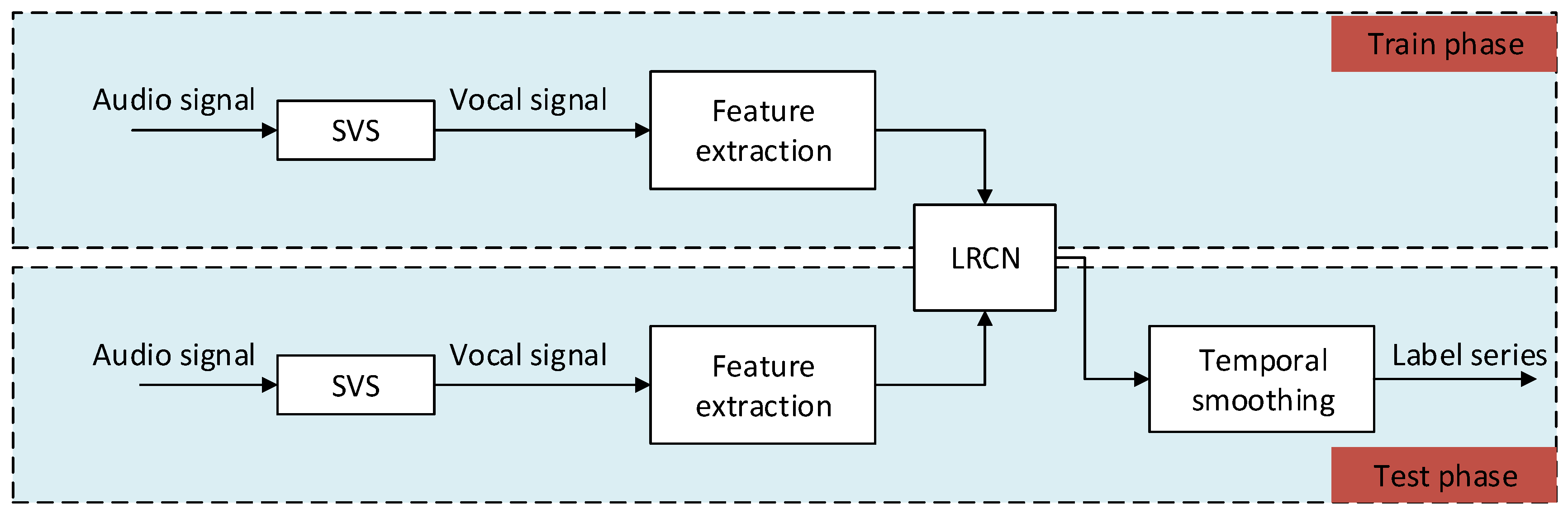
The architecture of the proposed system uses singing voice separation (SVS) as preprocessing to obtain vocal signals and then follows the conventional classification approach, where machine learning techniques (the LRCN) are applied to successive frames of input vocal signals with a set of audio features. Then, the output of the classifier is further processed by a smooth decision function. An overview of the proposed singing voice detection system is shown in
Figure 1. The different building blocks of the system are described in detail below.
3.1. Singing Voice Separation
Suppose that the goal of singing voice detection is to distinguish between a singing voice and silence instead of a singing voice and musical accompaniment. Then, simply using short-term energy can accurately locate all singing voice segments. The use of singing voice separation technology can eliminate or weaken the musical accompaniment to obtain a relatively pure human voice. Therefore, during preprocessing, a singing voice separation method is adopted to filter the original audio into a singing voice signal, while the accompaniment is filtered out.
There are many existing singing voice separation algorithms. According to related papers [
26], the most effective method for singing voice separation is based on U-net. U-net also uses a deep neural network, taking the spectrum as the network input for end-to-end model training. The U-net network structure proposed by Jansson et al. [
27] was reproduced, including six convolutional layers and six deconvolutional networks. The model was trained using three datasets: iKala (
http://mac.citi.sinica.edu.tw/ikala/), MedleyDB [
28], and DSD100 (
https://sigsep.github.io/datasets/dsd100.html). The training focuses on the spectrum of pure singing voices. In the presence of strong accompaniment, the original audio cannot be split clearly, and the separated vocal signal still contains harsh noise. After SVS, two versions of audio signals (i.e., raw audio and vocal audio) were generated for the same dataset to validate the effects of the preprocessing.
3.2. Feature Extraction
This section briefly describes the features used in the audio representation. Considering the ability of discrimination of vocal or music signals [
29], ZCR, MFCC [
25], LPCC [
30], Chroma [
31], PLP [
32], the first-order difference of MFCC, the second-order difference of MFCC, and the spectral statistical features [
33] (RMSE, centroid, roll-off, bandwidth, flatness, contrast, and polly) were computed. The spectra were also calculated as a raw feature to verify the performance of LRCN and its ability in fusing features.
The MFCC features have been widely used in many speech recognition and audio recognition problems [
6]. The most popular method for simulating human voice production is linear predictive coding (LPC), which performs well in clean environments but does not perform well in noisy environments. The LPCC feature is calculated by introducing cepstrum coefficients in the LPC parameters. It is assumed that the character of the LPCC is the nature of the sound produced depending on the shape of the vocal tract. The chroma feature is a valid tool for analyzing and comparing music data [
34]. By recognizing the different spectral components in musical octaves, the chroma feature exhibits a high degree of invariance with respect to timbre changes. The spectral statistic features represent the frequency information of the audio signal. The PLP is originally used for wrapping the spectra to minimize the difference between speakers and maintain the content of speech.
Feature vectors are calculated from the separated vocal audio signals. The features have been extracted for combining feature vectors concerning the high variability of the singing voice in vocal detection.
The audio signal is first divided into overlapping short frames. The audio signal sampling rate is 16,000 Hz, high-frequency limit 800 Hz, low-frequency limit 0 Hz. The frame size is set as 2048 samples (1.28 s), and the overlap size is 1536 samples (0.96 s). From each frame, a Hamming window is used to calculate the FFT. MFCCs are computed with 80 coefficients, and their first-order difference and second-order difference are computed as well. LPCC is computed with 12 coefficients. The chroma feature with 12 coefficients is included. The PLP has nine coefficients. All spectral statistical features together have 15 coefficients. Finally, the combined feature vector has 288 coefficients.
3.3. LRCN for Classification
This paper proposes a new data-driven singing voice detection method based on LRCN [
23]. The motivation behind using LRCN is its ability to learn both spatial and temporal representation. Not only the long-term dependencies between inputs but also more efficient information from convolution could be combined with the final representation.
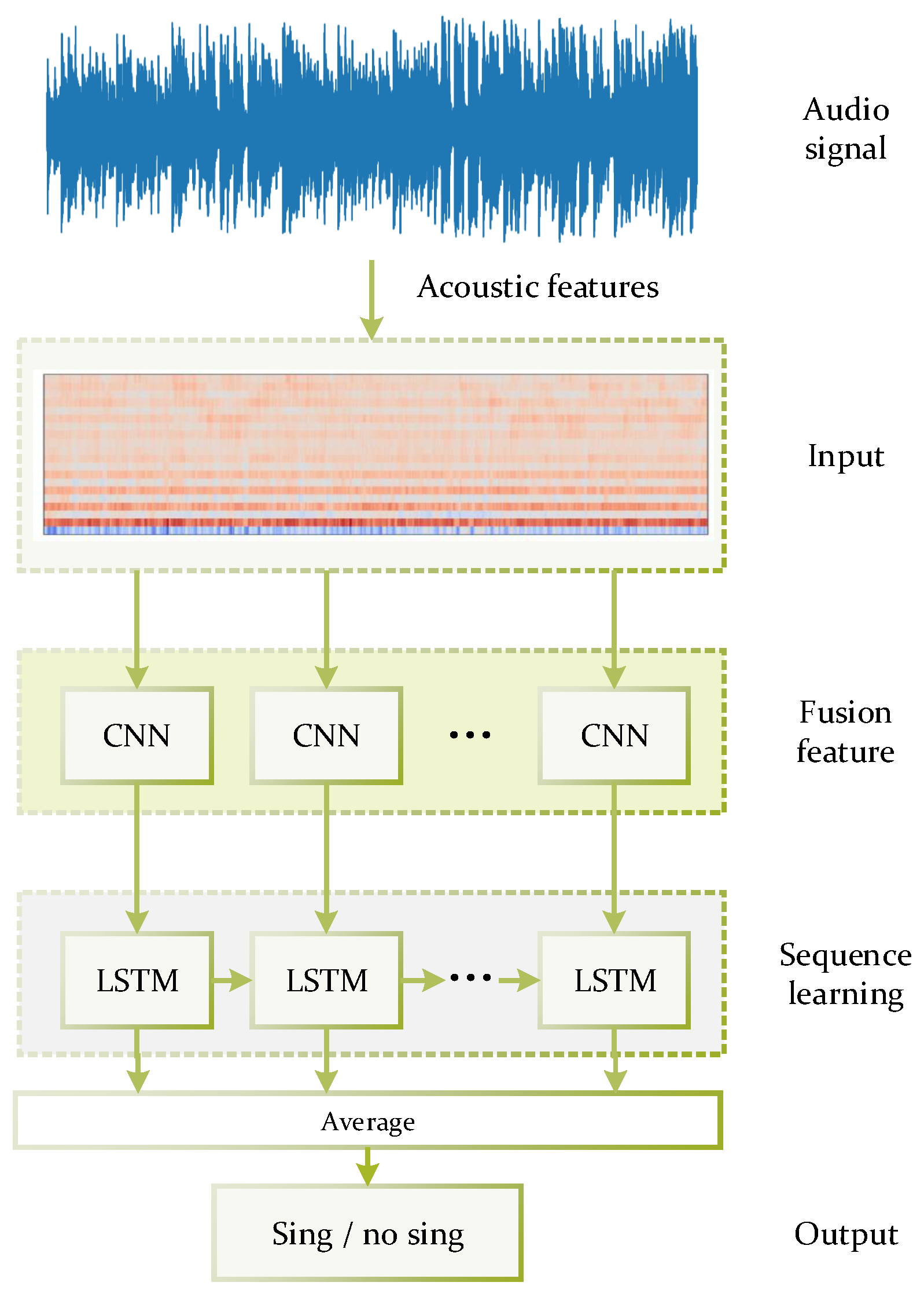
The network for singing voice detection has an input layer that matches the size of the combined acoustic feature vector, three hidden layers, and an output layer with a single sigmoid unit. The network is trained as a classifier to output vocal scores for each frame block in a value space of 0 and 1, where 1 indicates singing voice and 0 indicates no singing voice. The neural network topology is shown in
Figure 2.
The LRCN model combines a feature extraction CNN with an LSTM model, which can learn to identify and synthesize the temporal dynamics of tasks involving sequential data.
Figure 2 shows the core of the LRCN based system, which works by passing the fusion features of successive audio frames to learn a new vector representation. The input audio signals are preprocessed by singing voice separation. After the feature representation, the sequence model LSTM takes over.
The output of LSTM depends on the hidden state in the previous time step and the weights. Therefore, the vector representation after CNN also must be performed in sequence.
The final step in predicting the audio frame at time step t is to take the softmax and then temporally smooth the output of the sequential model.
During the training of the LRCN model, the batch size is 32, learning rate is 0.0001, drop-out rate is 0.2, number of epochs is 10,000, and early stop is used. The parameters of the deep model are listed in
Table 1, where the LRCN layer contains a stack of one-dimensional inputs with a set of one-dimensional kernels. There is a max-pooling layer subsampling a stack of one-dimensional inputs by taking the maximum over small groups of neighboring frames. In the input layer of the networks, combined features of the successive frames in a fixed block size are fed for training.
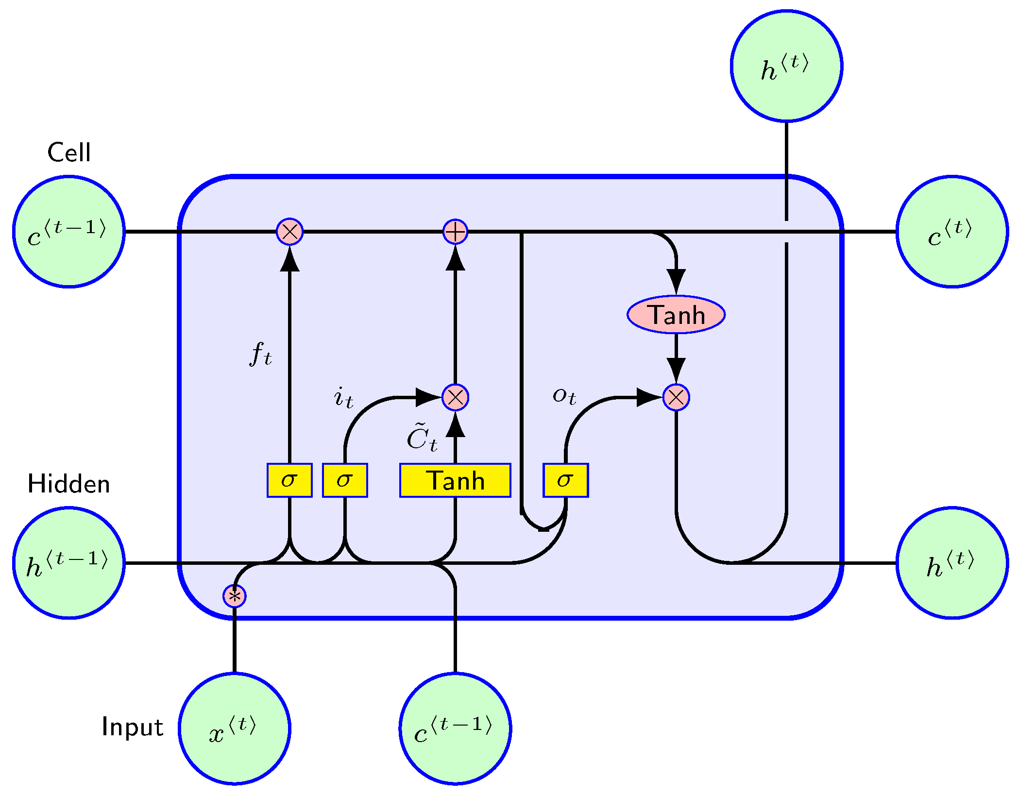
The input data are concatenated on successive frames. The input vector of successive frames is finally mapped to one label based on the ground truth. In the LRCN layer, 256 convolution filters are used, and the convolution kernel with a shape of (1,4) operates a one-dimensional convolution along with the different feature dimensions. The LRCN layer determines the future state of a certain cell in the grid of the input and past states of its local neighbors [
35]. This can be easily achieved by using a convolution operator in the state to state and input to state transitions. The inner structure of LRCN is shown in
Figure 3. The key equations are shown in Equations (
1)–(
5).
where “·” represents the element-wise product, and “
” represents the convolution operator.
is the sigmoid function,
W is the weight matrix, and
b is the bias vector. The input gate
, forget gate
, and output gate
of LRCN are separately listed in (
1), (
2), and (
4). The
shown in Equation (
3) is the LRCN cell, and
in Equation (
5) is the output of the LRCN cell. All inputs, cell outputs, hidden states, and gates of the LRCN are 3D tensors.
3.4. Postprocessing
The frame-wise classification changes very quickly, and the likelihood ratio changes from frame to frame. Compared with the label data, the category of consecutive frames remains unchanged in the label data. Given the continuity of singing in music over a certain period of time, accumulating segment likelihood over a longer period is more reliable for decision making. Thus, the audio signal is segmented into long blocks. Within each block, the feature mentioned above will be calculated from frames. The block is then labeled according to singing and nonsinging.
Three methods of segmentation smoothing are applied to singing voice detection. One is the median filter, which simply smooths the original categorical variable along the time dimension, which can essentially replace the value of each frame with a weighted average of the values over a wider window. The second method is to use the result of posterior probability with an HMM with two states (vocal and nonvocal). The observation distribution is fitted by 45 Gaussian mixture models and is fitted with the expectation-maximization algorithm. It then uses the Viterbi algorithm to obtain the best state path from the output sequence of the classifier. The third method is a conditional random field (CRF), which is a supervised model. CRF is trained on the validation dataset to model the relation between the prediction and the ground truth.
4. Experiment and Results
For comparison, five public datasets are mainly used in the related works of singing voice detection. The binary classification evaluation metrics of recall, precision, accuracy, and f1 measure are used.
Experiments were conducted with the five public datasets, including the use of singing voice separation as the preprocessing, and both vocal data and raw data were compared to train networks. The performances of different features and their combinations were then compared. Frame window size and block size were tuned to decide the input sequence. Different temporal filtering techniques were compared to the postprocessing. Finally, a comparison with the state-of-the-art singing voice detection system on the public datasets is provided.
4.1. Benchmark Datasets
The Jamendo Corpus includes a group of 93 songs with Creative Commons licenses from Jamendo’s free music sharing website, constituting approximately 6 h of music in total. Each file is manually annotated with singing and nonsinging parts by the same person to provide ground truth data [
14]. Jamendo audio files are encoded in 44.1 kHz stereo with a bit rate of 112 kb/s with Vorbis OGG (or 128 kb/s for MP3 files). In this experiment, each file was converted to mono in WAV format. The entire dataset is divided into three nonoverlapping sets, a training set, a validation set, and a test set, consisting of 61, 16 and 16 songs, respectively. Since 50.3% of the frames are singing segments, and 49.7% are nonsinging segments, the entire set is well balanced.
The RWC popular music dataset contains 100 popular songs, with annotations by Mauch et al. [
12]. RWC contains 80 Japanese pop songs and 20 English pop songs, each of which was annotated by the audience. The audio file has a sampling frequency of 44.1 kHz, a stereo channel, and 16 bits per sample. In our experiments, the files were converted to mono. Since 51.2% of the frames are singing segments and 48.8% are nonsinging segments, the entire collection is very balanced. Since the original dataset did not have a subset split for training and testing, 4-fold cross-validation was performed. The entire dataset was divided into four nonoverlapping collections, each of which included 25 songs. Each song was used four times as a testing subset in turn, and the other three were used as a training subset for model training. The validation set is separated from the training set, accounting for 20%.
The MIR1k dataset contains 1000 singing voice clips, where the left and right channels are music and vocal signals, respectively. To avoid same song being divided into different datasets, according to the principle of no-overlap recordings, the dataset was split into training, testing, and validation with the ratio of 8:1:1. The labels of vocal and nonvocal were calculated according to the right channel with energy detection and the energy threshold is calculated by the average of random selected non-vocal frames. In the testing phase, the right channel and the left channel were mixed to the mono channel.
The iKala dataset was built by professional singers. Just as with MIR1k, the left channel and right channel are music and vocal signals, respectively. There are a total of 252 30-second excerpts. The labeling and dataset splitting methods are the same as the processes of MIR1k.
The MedleyDB dataset contains 61 tracks with vocal signals that include annotations of melody. The vocal and nonvocal labels are acquired according to the pitch value, where nonzero pitch is labeled as vocal and others are labeled as nonvocal.
4.2. Evaluation
The experiments were mainly conducted on both Jamendo and RWC, and the results of the related works on these two benchmark datasets were respectively compared. To provide a comprehensive view of the results, model predictions were compared with the ground truth labels to obtain the number of false negative (FN), true negative (TN), false positive (FP), and true positive (TP) results accumulated over all songs in the testing set. The frame-wise recall, accuracy, precision, and f1 measure were calculated to summarize results. The four metrics can be represented in the following formulae:
4.3. Results
Five experiments were conducted in total. The first involved preprocessing with singing voice separation to verify the effectiveness of singing voice separation as preprocessing. The second involved different audio features and their combinations as input with the proposed LRCN method for feature fusion. In the third experiment, the frame size and block size of successive frames for the input layer were tested. In the fourth, the three different methods of temporal smoothing for postprocessing were compared. In the last experiment, comparison with the state-of-the-art singing voice detection system is provided.
4.3.1. The Effects of Singing Voice Separation
In the first experiment, the vocal signal was separated from the raw audio signal. The combined features were extracted to train the LRCN model. The model had an input shape of (1, 1, 20, 276), where the third dimension is the time step used for LSTM, the fourth dimension is 276 not 288 because the final selected features did not contain the feature of Chroma (12), and the detailed parameter configuration of the deep network is shown in a Gitlab repository (
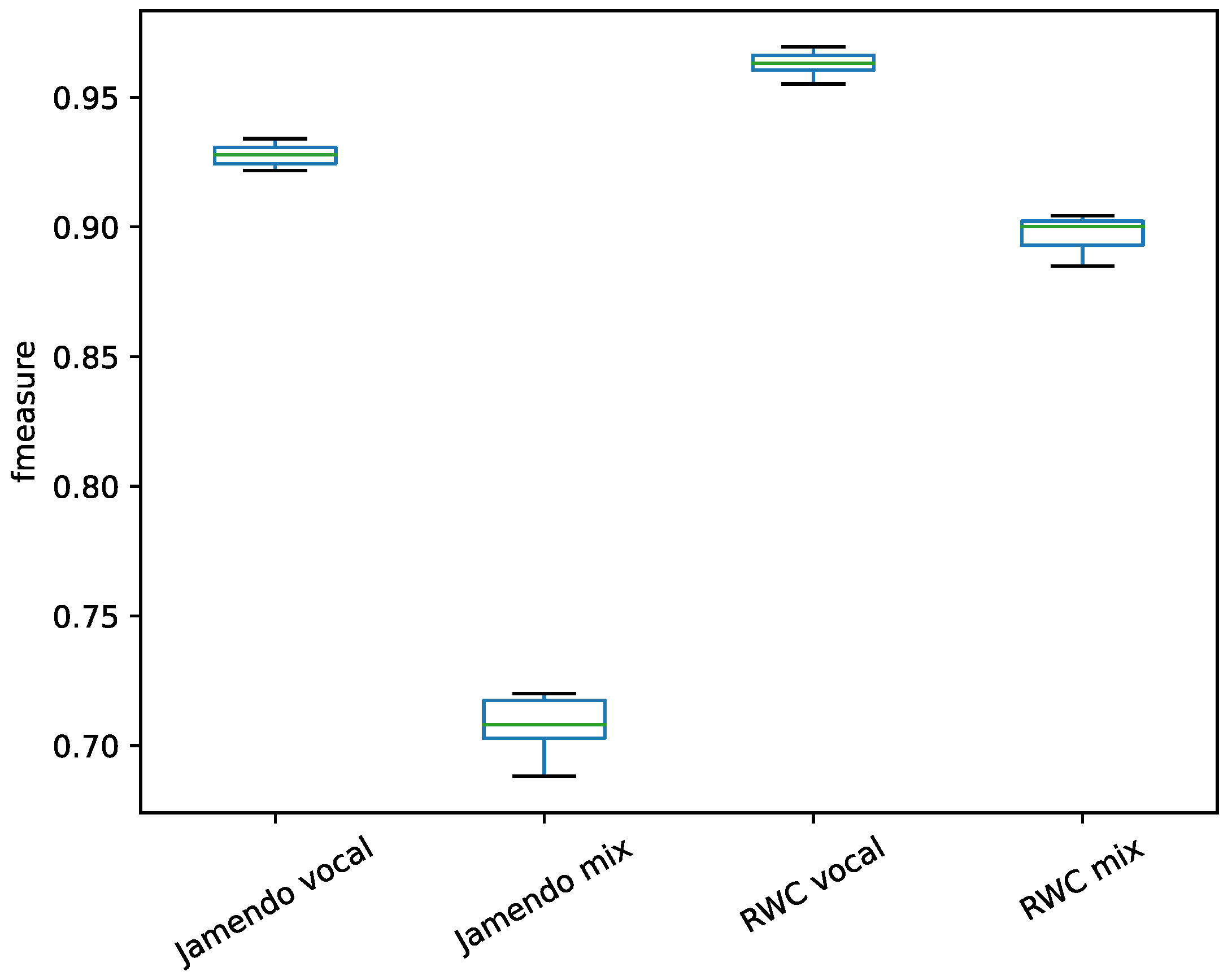
https://gitlab.com/exp_codes/svd-review). The binary classification results were compared on the split vocal and the raw mixed audio. The performances on the vocal data and raw audio data are shown in
Figure 4.
From the comparison of the classification results using different audio signals on two datasets, the use of separated vocal signal exceeds the raw mixed signals in terms of f-measure, so the application of the preprocessing of singing voice separation can improve the singing voice detection performance. The difference for Janmendo dataset was more pronounced than that observed for RWC dataset. The difference was caused by the different music, although with the same preprocessing of singing voice separation, the vocals separated from Jamendo dataset are clearer than those of the RWC dataset. In the song, the accompaniment is often strong and is not only temporally overlapped with the vocal signal but also intertwined with the vocal signal in frequency. The preprocessing of singing voice separation can thus degrade the influence of the accompaniment and improve feature representation.
4.3.2. Comparison of Performance with Different Features
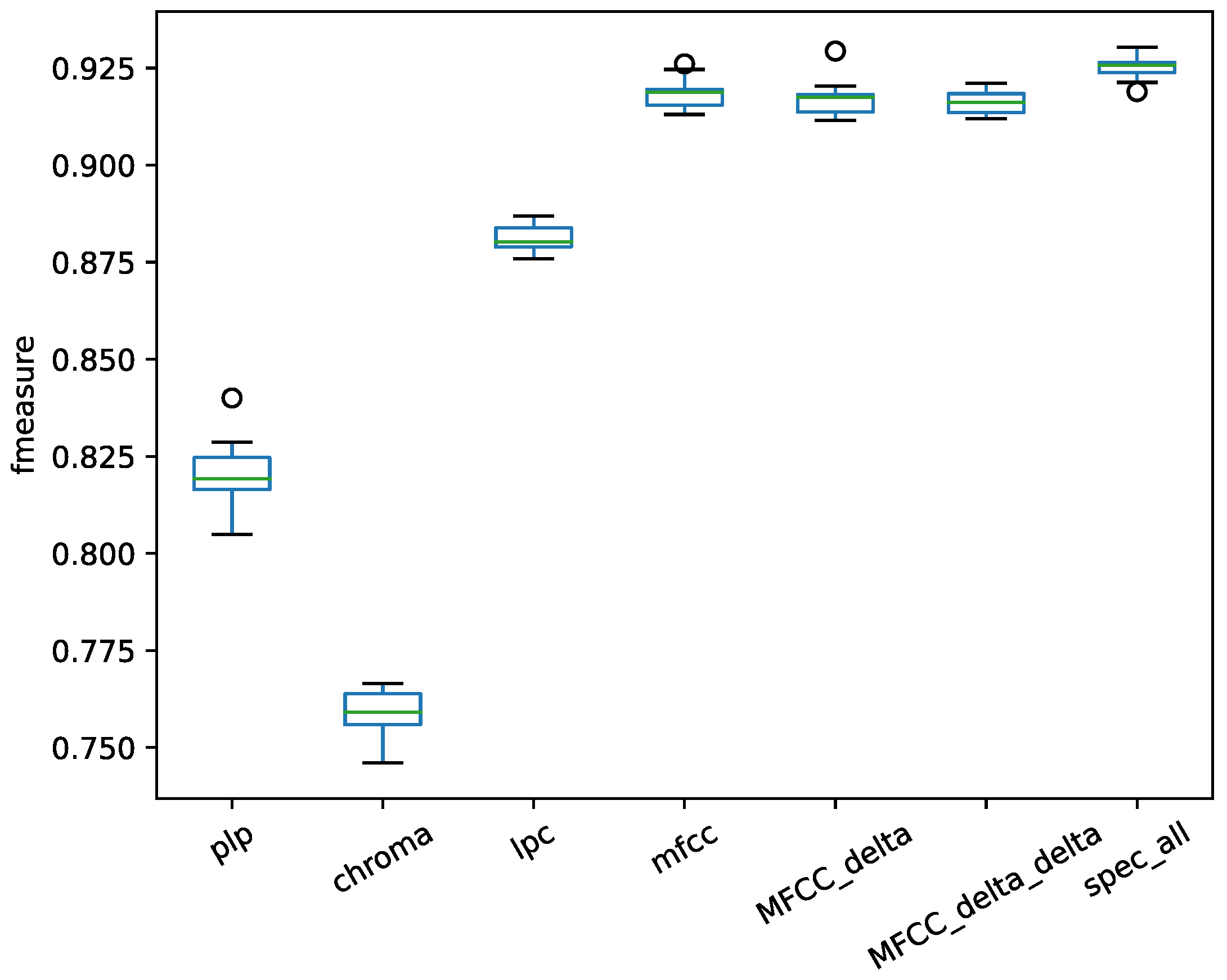
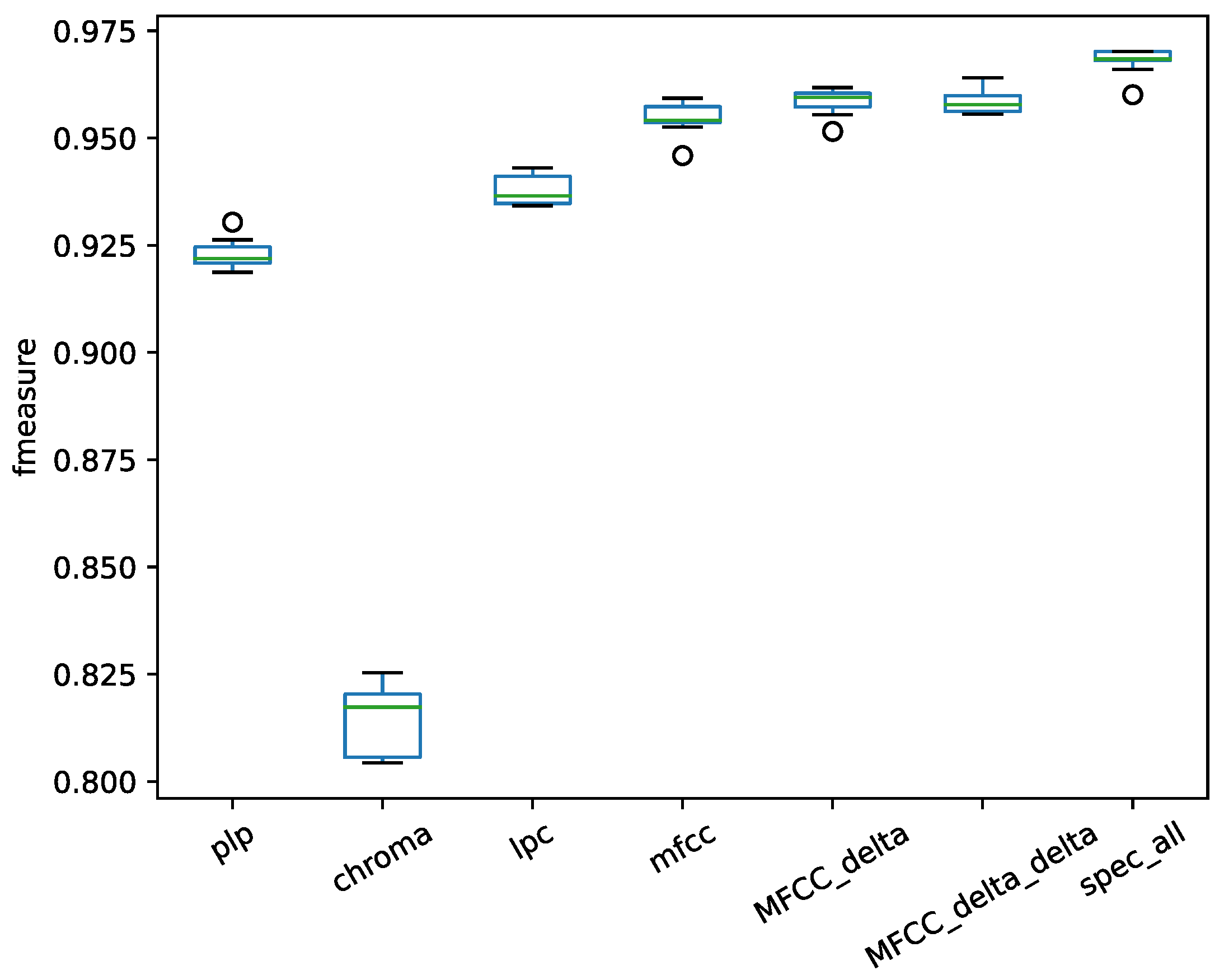
From speech processing to music information retrieval, many audio descriptors have been introduced to the field of singing voice detection. The combined features were used to classify the vocal and nonvocal segments with the deep LRCN model. The performances of the features on the separated vocal signal of the Jamendo dataset are shown in
Figure 5, with the RWC dataset results in
Figure 6.
From the results of different features in
Figure 5 and
Figure 6, the chroma feature exhibits poor performance for the task of vocal detection, and the spectral statistical feature achieved the best performance. The different feature sets were concatenated in each frame. Through the LRCN model, a deep feature was extracted with the convolution layer.
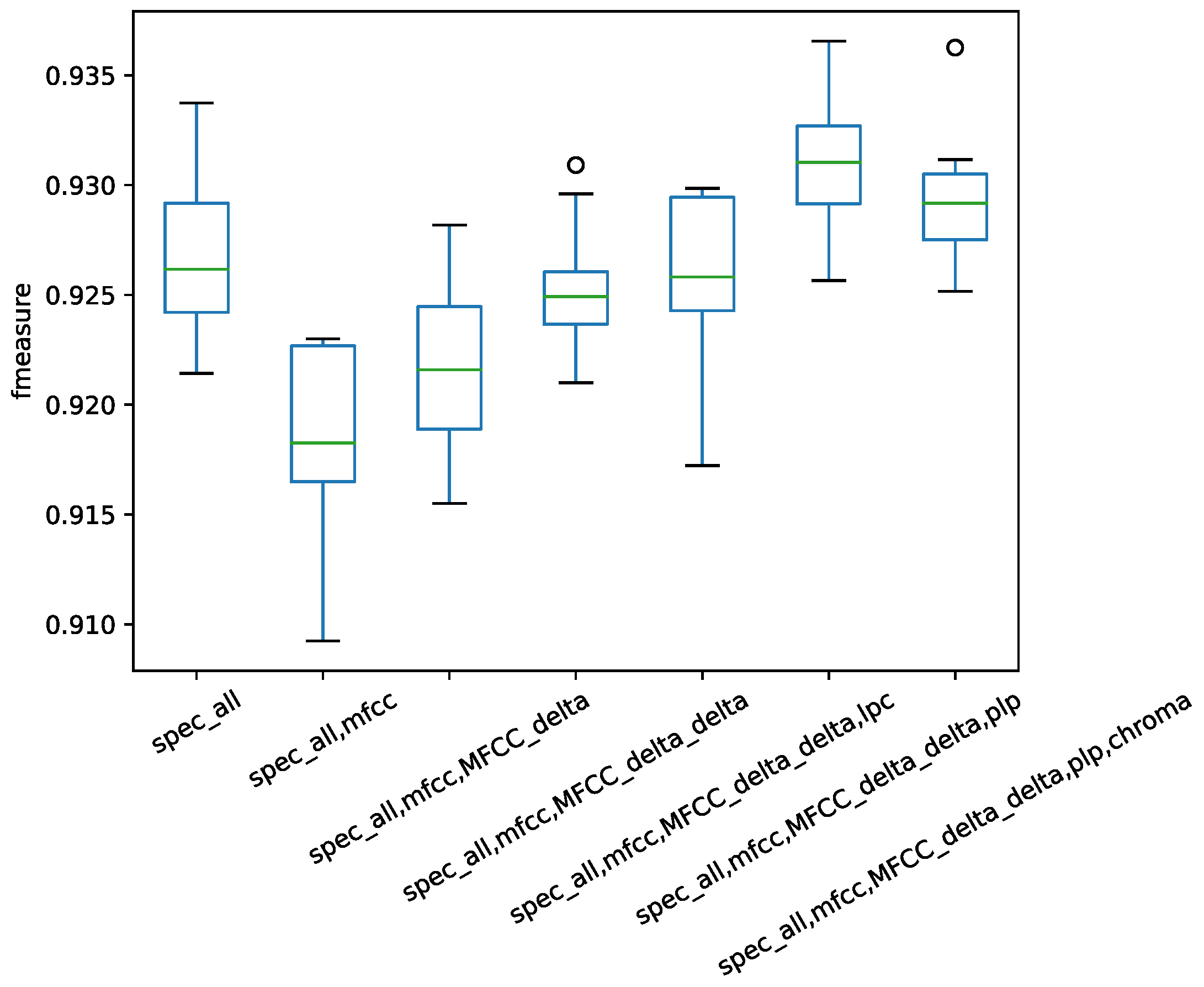
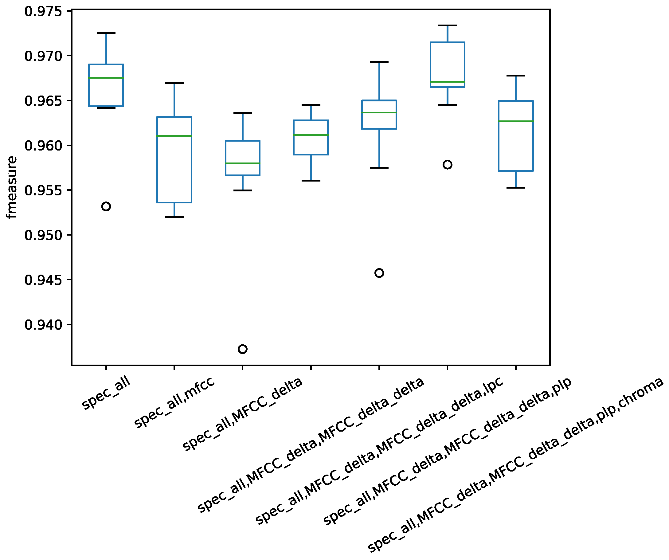
To determine the best feature combination, according to the performance of a single feature, each subfeature was added into combined features one by one. The first added was the spectral statistic feature with the highest f1 measure. The combination results are shown in
Figure 7 for the Jamendo dataset and in
Figure 8 for the RWC dataset.
From the feature combination results for the Jamendo dataset shown in
Figure 7, the spectral statistic feature, MFCC, and the second-order difference of MFCC and PLP together is the combination that achieved the best performance. For the RWC dataset, the best combination was the spectral statistic feature, the first-order difference of MFCC, and the second-order difference of MFCC and PLP. With the observations on the two datasets, the combined features were set as the spectral statistic features, PLP and MFCC.
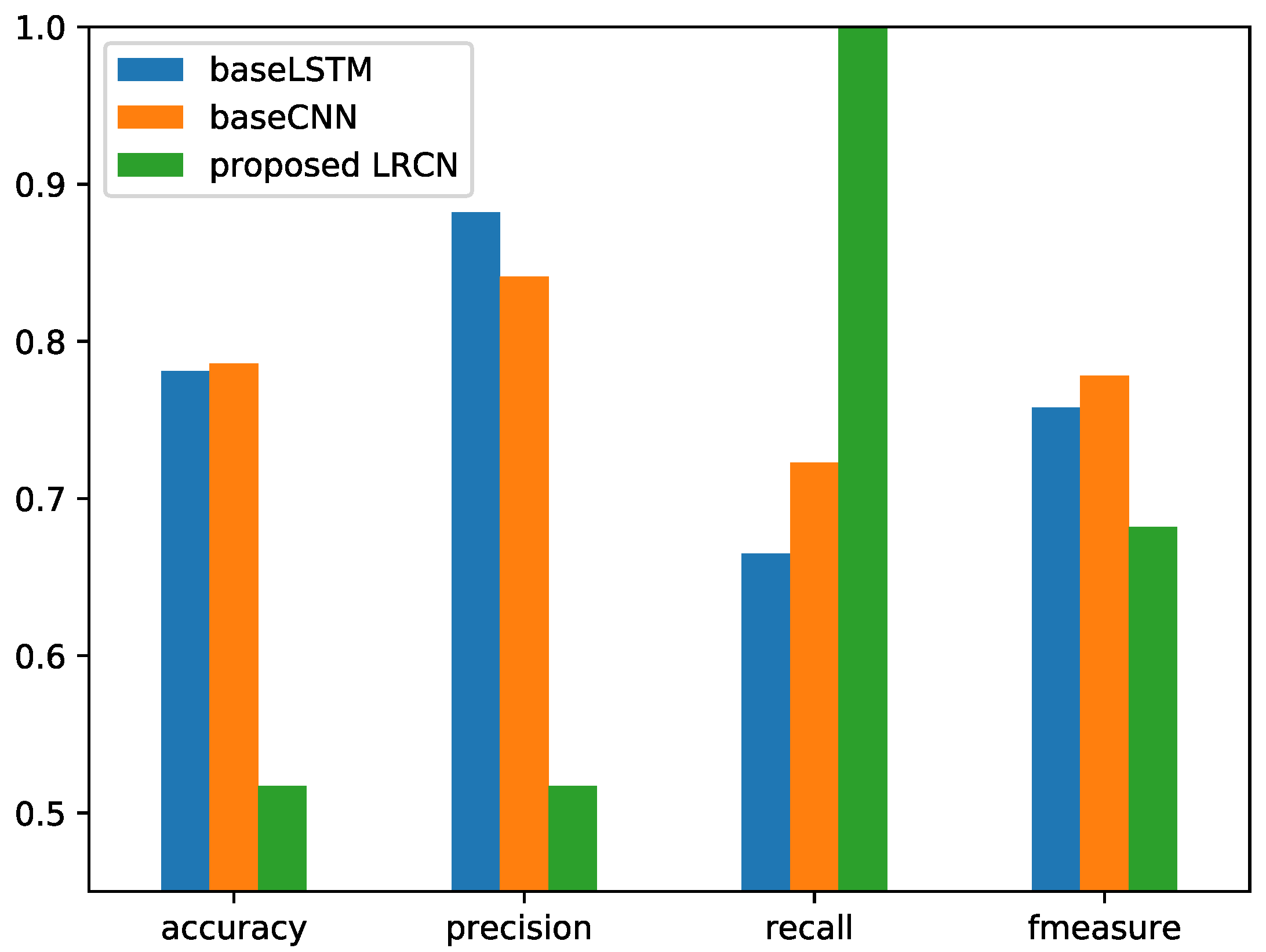
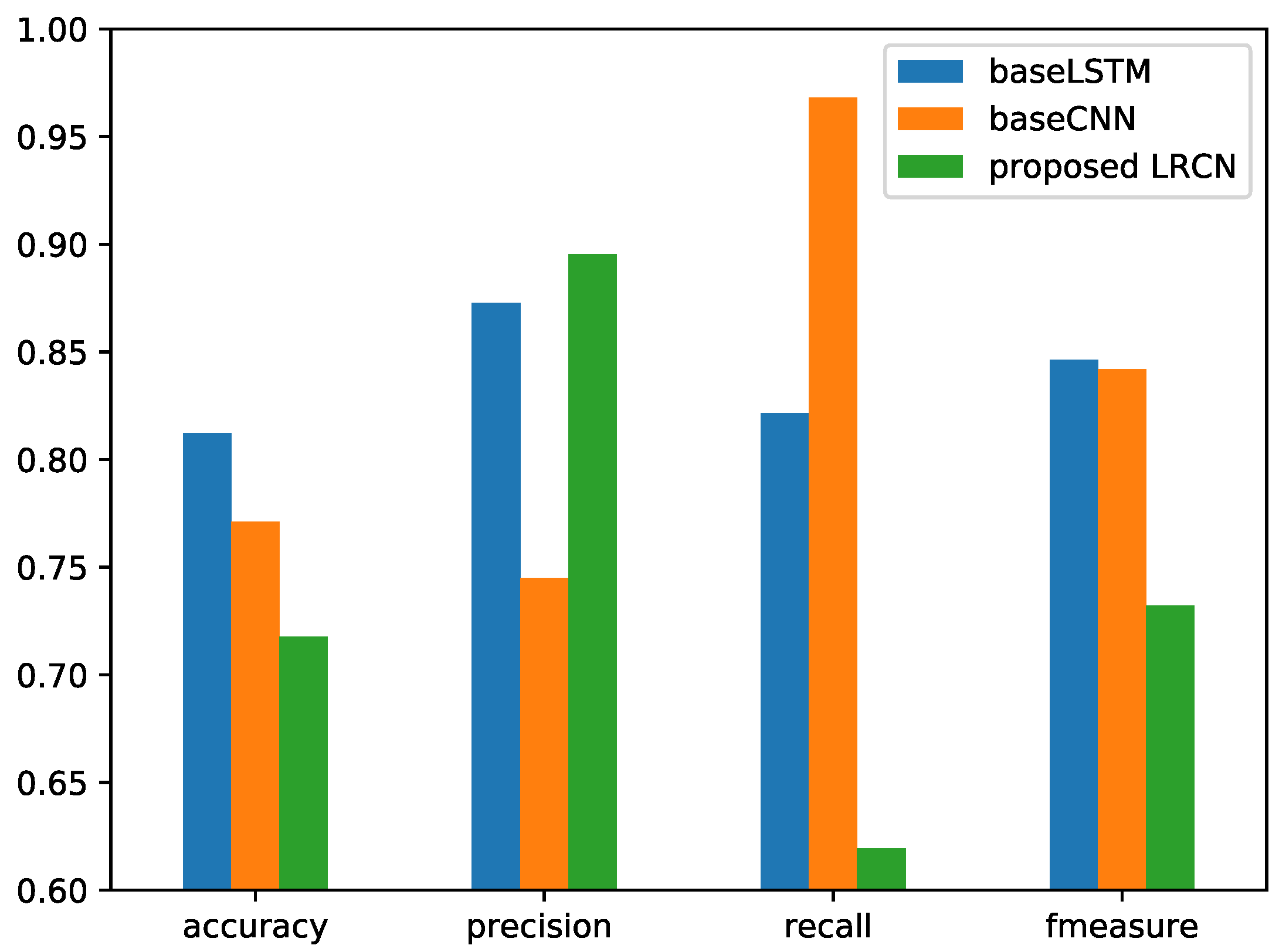
Differently from handcrafted features, the spectrum was obtained from the audio signal through Fourier transform and contains more comprehensive information. With the spectrum as the LRCN input, an end-to-end feature was extracted. The spectrum of the successive frames in a fixed-length block was fed to the LRCN. Since the proposed LRCN method is a combination on the basis of LSTM and CNN, the frequency spectrum was used as the input, and the proposed LRCN was compared with the baseline method LSTM (baseLSTM) and CNN (baseCNN). The comparison details are listed in
Figure 9 for the RWC dataset and
Figure 10 for the Jamendo dataset.
Through the results shown in
Figure 9, the spectrum as an input feature for LRCN has a weak ability to distinguish vocal and nonvocal signals. When the spectrum included larger dimensions of 513, the model did not effectively learn from the spectrum in the cases of the two public datasets. The comparison method based on LSTM also could not produce the best performance with the spectrum as input. Owing to the large spectral dimensions and the small dataset, especially the Jamendo dataset, the model was nearly over-fitted in the training phase, and nearly identified all frames as accompaniment. On the other hand, when adding CNN into a single frame, the frequency information was fused. The fused features obtained by LRCN cannot distinguish between vocal and nonvocal signals.
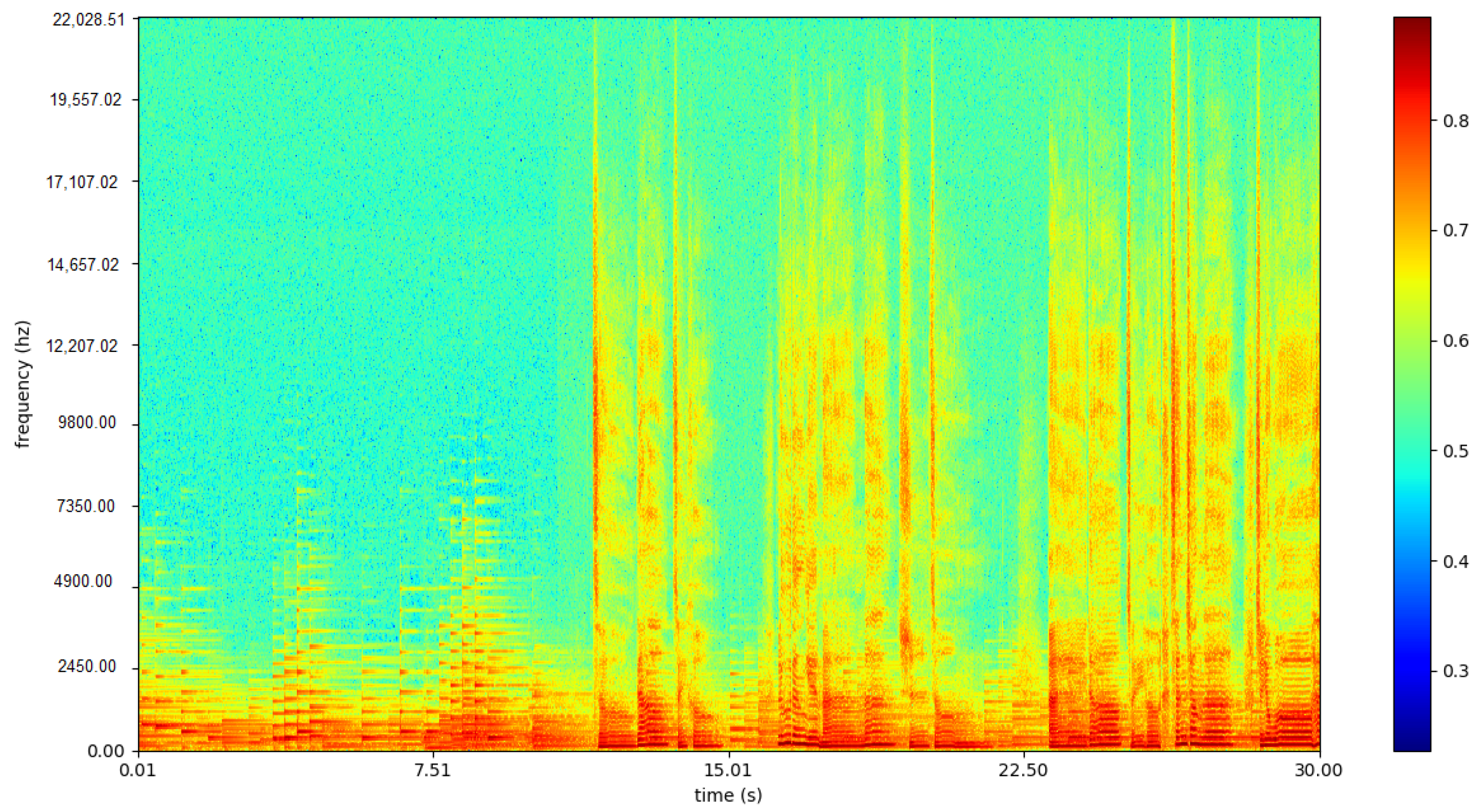
The comparison of spectrum of the vocal signal and accompaniment from the same song provided by the iKala dataset are shown in
Figure 11 and
Figure 12. With the one-dimensional convolution and one-dimensional max pooling on each frame, the fused spectrum feature ineffectively distinguished between singing and nonsinging.
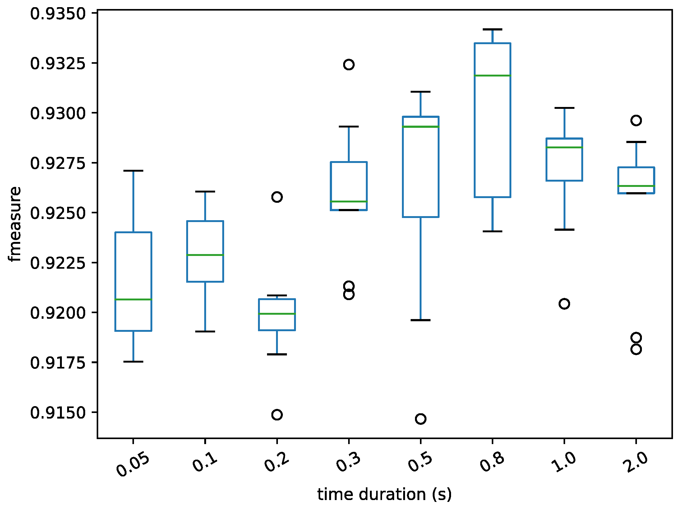
4.3.3. Frame Size and Block Size Setting
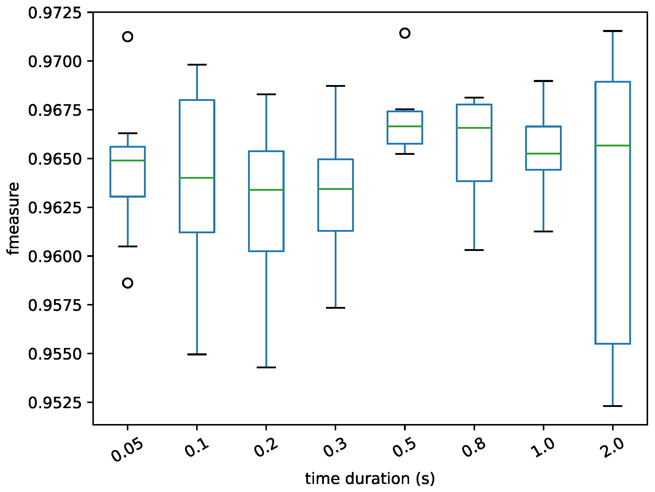
During the feature extraction, the frame size was valid for the two datasets.
Figure 13 and
Figure 14 show the performance with frame size ranging from 50 ms to 2 s and the horizontal axis is time.
It can be seen from the experimental results that the duration of the frame has a certain effect on the results. Through observing
Figure 13 on the Jamendo dataset, it was found that when the frame length was set to 0.8 s, the average value of the experimental results was optimal, but the maximum and minimum fluctuations were relatively large. Although the average value of the experimental results was slightly lower when the duration of the frame is set to 1 s, the fluctuation range was also small. Similarly, the results on the RWC dataset in
Figure 14 also reflect the small fluctuation range for when it was set to 1 s. Therefore, the frame length was set to 1 s, as the performances were consistent in those two datasets.
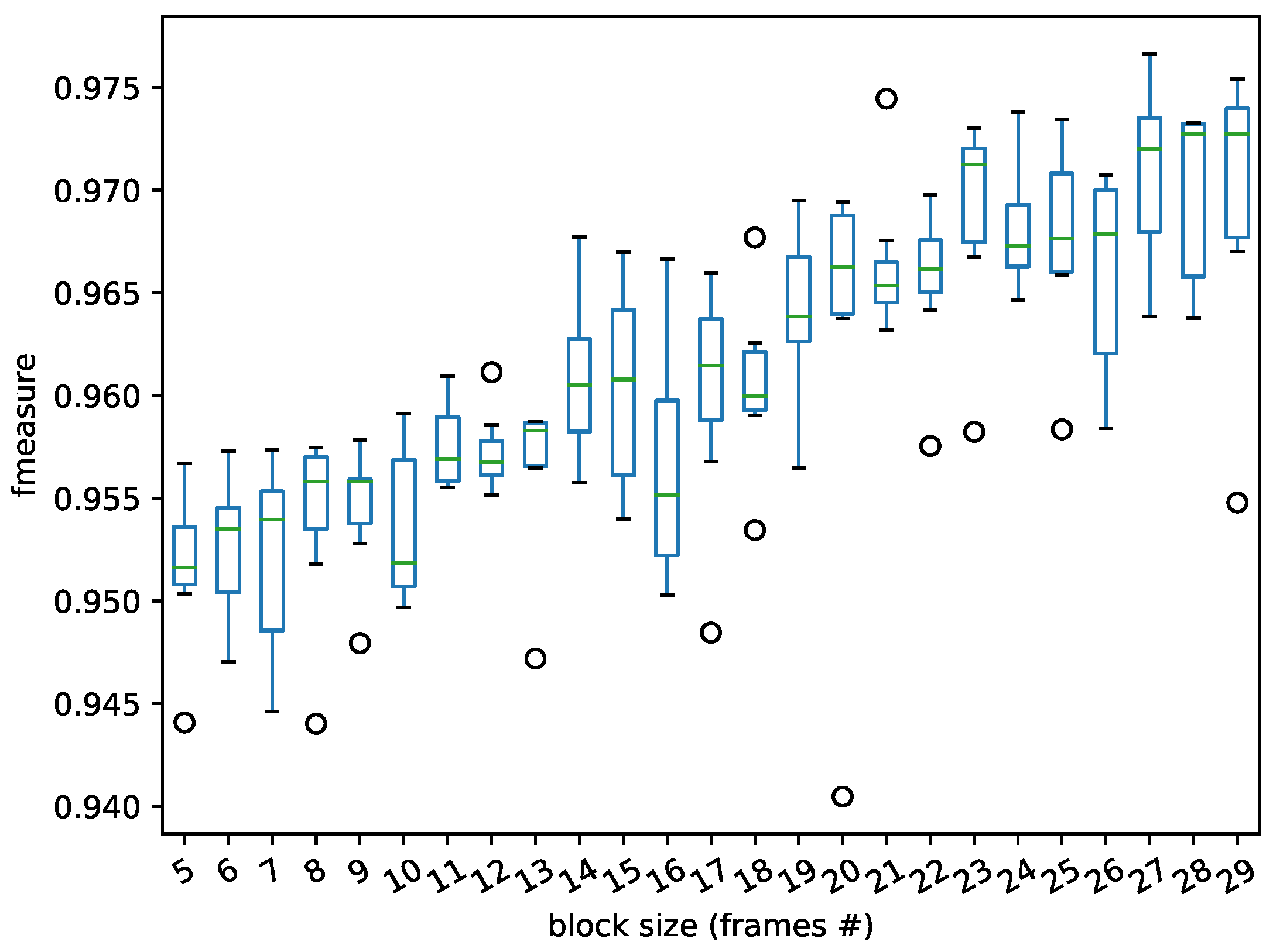
The input frame-block size decides the input sample number.
Figure 15 and
Figure 16 show the performance with the block size settings used for the LRCN feature input layer varying from 5 to 29 and the horizontal axis is the number of frames. The time steps of the LRCN model served as the control variable for the two datasets (Jamendo and RWC).
From the results in
Figure 15 and
Figure 16, the effect of block size setting in the LRCN model on the vocal detection fluctuates slightly. Through the experiments, 20 frames were selected as input for the LRCN model.
4.3.4. Comparison of the Different Temporal Smoothing Methods
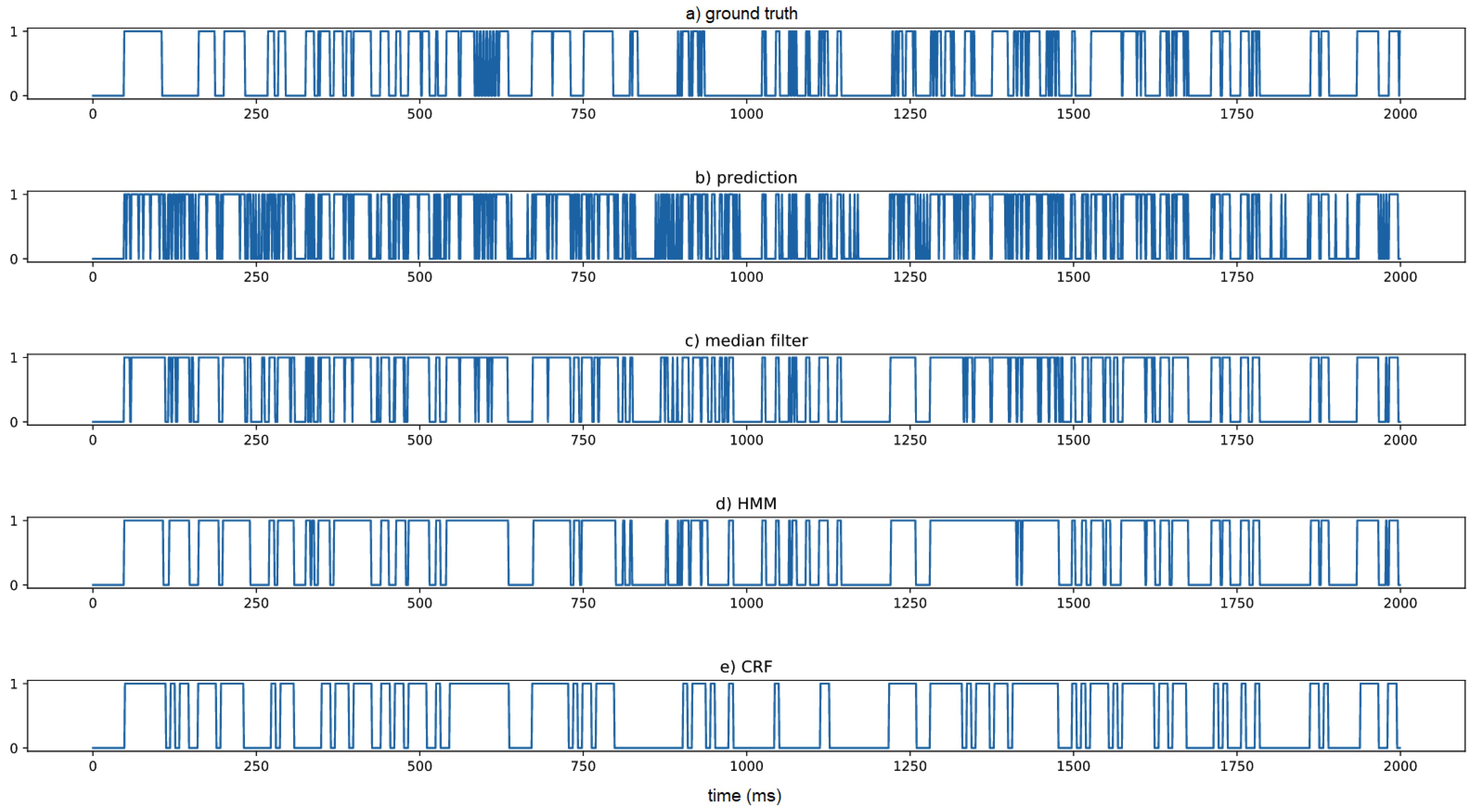
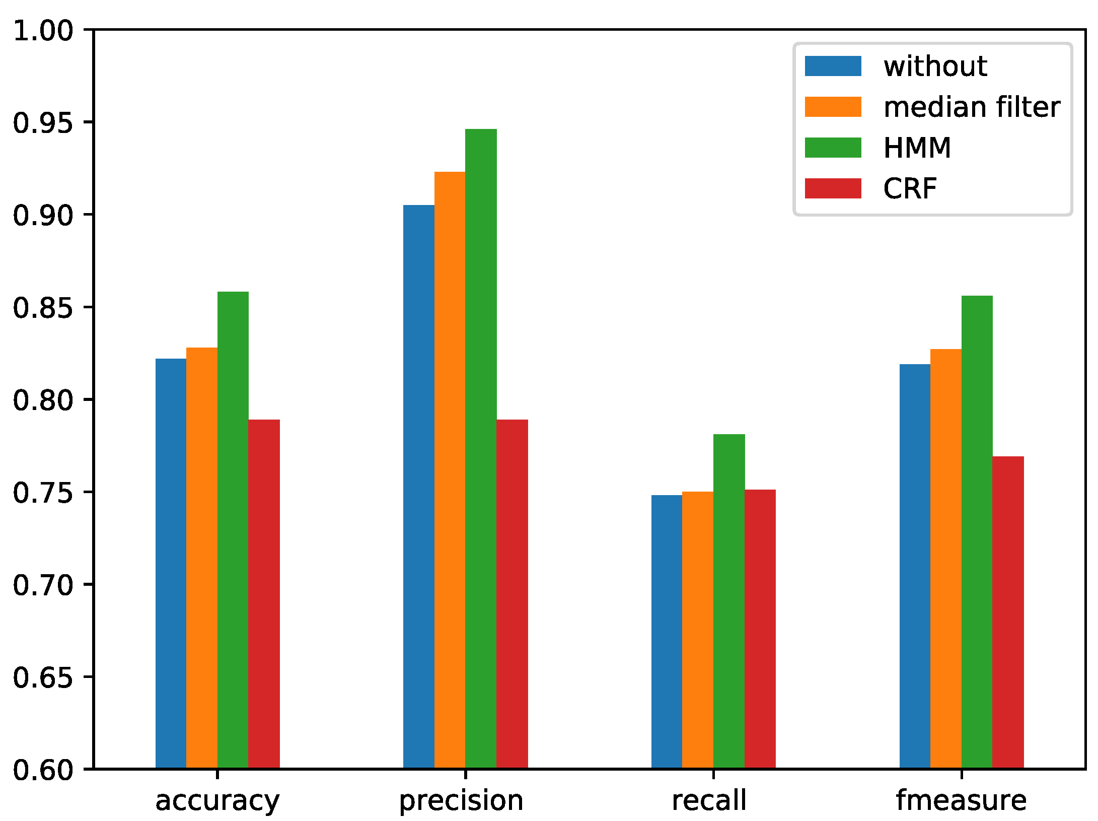
In the postprocessing, three temporal smoothing methods were compared. Median filtering for temporal smoothing was used to modify the frame prediction error in a block with a fixed block size. The block size includes various choices and can be decided by experimentation on the validation dataset. As for the second temporal smoothing method, HMM was used for the predicted probability. Unlike the median filter with fixed block size, the HMM-based method can learn from the probability series without manually choosing parameters. The predicted probability of the LRCN model was used. Given a probability sequence, a two-state HMM was trained. At the end of the training process, considering the linear time complexity, the dynamic programming method Viterbi was used to obtain the sequence with the largest probability. HMM predicts the segment boundary, and then, each segment votes for the final label. The third one was CRF, similar to HMM, which is a discriminative model rather than a generative model. The trained CRF model was also used to smooth the label series, and the three postprocessing methods were finally compared with the ground truth segmentation. Segmentation with different methods is shown in
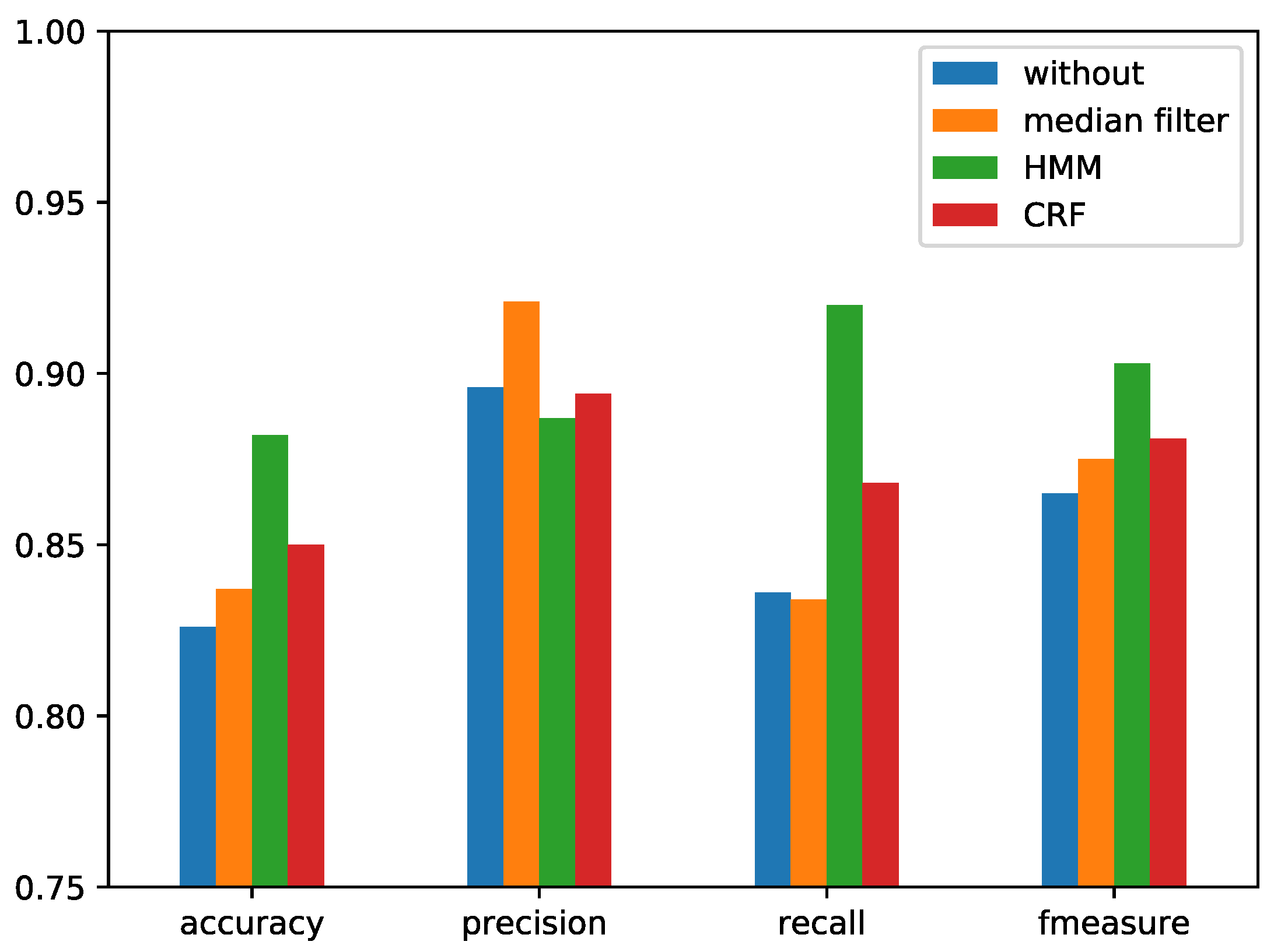
Figure 17 and the horizontal axis is time. The performances with different postprocessing methods are shown in
Figure 18 for the RWC dataset and
Figure 19 for the Jamendo dataset. Here, the LRCN model was used with the combined features.
From
Figure 17, the raw prediction by the model includes many small segments and varies frequently. After the temporal smoothing as postprocessing, the segments are more consistent with the ground truth segments.
From the comparison results shown in
Figure 18 and
Figure 19, the postprocessing is necessary for the frame-wise singing voice detection system. The performance of singing voice detection was improved 4% by HMM. The performances of median filtering and CRF based methods were inferior to the HMM-based method. Median filtering smooths the sequence in a fixed window, which leads the original boundary to disappear and generates new fixed-length segments. The use of median filtering will produce false positives, so the recall becomes smaller. The CRF model needs the data sequence to be split into parts. Although there is no need to set each part as a fixed length in the training phase, there is also a boundary problem for the window length that needs to be set in the training phase. The length being either too small or too long will lead to inconsistencies in training and testing.
4.3.5. Comparison of the Base Method under the Same Conditions
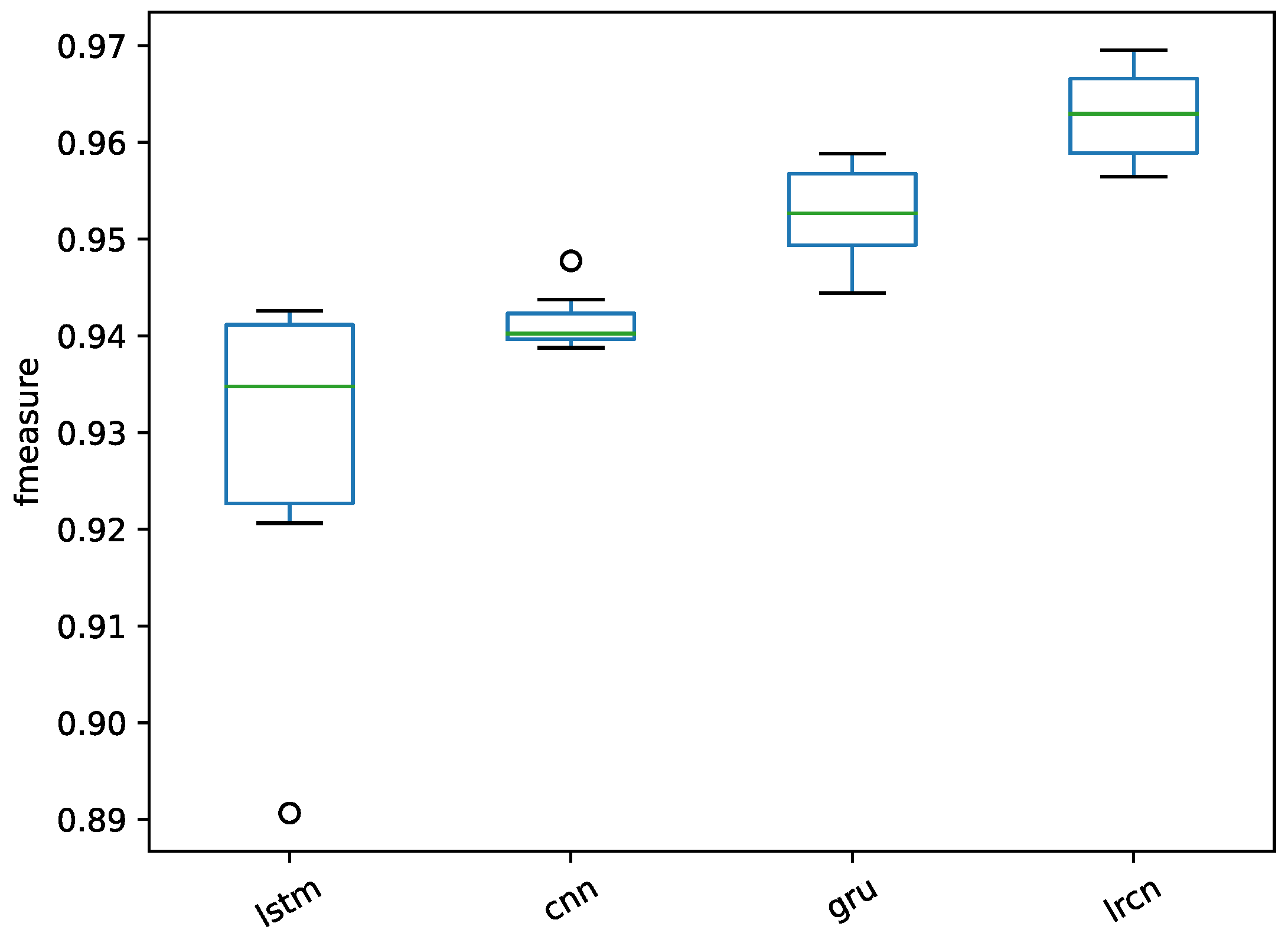
The proposed singing voice detection system is mainly based on the model of LRCN, which is the combination of CNN and LSTM. The models were compared with the same conditions of preprocessing and postprocessing on the respective Jamendo and RWC datasets in this experiment.
The two baseline methods CNN and LSTM were implemented to compare the performance of the LRCN. Just as in LSTM, a GRU was also implemented for comparison. The CNN model has four layers: the input layer for successive frames in a fixed duration, which is the same as the settings of LRCN; a convolution layer; then a max-pooling layer; and finally, a flatten layer connected to the output layer. It should be noted that the same frame-wise combined features were also implemented. The LSTM model was implemented with three layers: an input layer with the same frames as those of LRCN, a hidden layer, and finally, an output layer with a sigmoid unit. The experimental results are shown in
Figure 20 for the Jamendo dataset and
Figure 21 for the RWC dataset.
The results show that the performance of the LSTM with the combined features achieved a lower value of the f-measure than the CNN, the GRU, and the proposed LRCN. Without a deep feature extracted by the convolution layer, the multiple dimensions of different features cannot function effectively. The convolution on the combined multidimensional features can learn the relationship between different dimensions. With the comparison of the CNN and LRCN, the score of the f-measure has been improved by LRCN on the two datasets. The LRCN with the combination of CNN and LSTM can thus learn both the relation between different dimensions and the temporal context.
4.3.6. Comparison with the Related Works on Public Datasets
To further validate the proposed singing voice detection system, five datasets including Jamendo and RWC dataset were used. The averages of 10 prediction results are listed in
Table 2.
The proposed method performed well on the two benchmark datasets, RWC and Jamendo. On the datasets of MIR1K and iKala, the proposed method achieved 0.89 and 0.99 f1 values, respectively. The two datasets have the same method for tagging: the difference lies in the singing voices. The voices from iKala are more stable in pitch than the voices from MIR1K. From the results of MedleyDB listed in
Table 2, there remains room to enhance the singing voice detection. The labels generated according to the pitch value on the MedleyDB dataset exhibit certain misjudgments.
Finally, the proposed singing voice detection system was compared with the implemented LSTM, CNN, GRU and Ramona [
14], Schlüter [
19], Lehner-1 [
13], Lehner-2 [
16], Lehner-3 [
10], and Leglaive [
18] on the Jamendo corpus, and compared with Mauch [
12], Schlüter [
19], Lehner-1 [
13], Lehner-2 [
16], and Lehner-3 [
10] on the RWC pop dataset. The comparison results are shown in
Table 3 and
Table 4.
The proposed method was labeled as LRCN, and the baseline methods LSTM and CNN were implemented for comparison in this experiment. The same preprocessing and postprocessing were both added to LSTM and CNN. The three methods ran through 10 rounds prediction on test datasets and the average prediction results were used for comparison.
Table 3 shows the comparison of the experimental results on the Jamendo dataset. The LSTM and LRCN were both implemented with Keras 1.2.2 (
http://faroit.com/keras-docs/1.2.2/) on a GPU. The other six results were obtained in the related reports on the public dataset Jamendo with the same conditions. When compared with shadow models, the SVM of Ramona and the random forest of Lehner-2, the proposed LRCN achieved 0.927 in terms of f1 measure, which is higher than both models by about 9%. When compared with the classifier based on LSTM, the proposed LRCN outperformed the bi-LSTM of Leglaive and LSTM of Lehner-3 and got an improvement of about 2% in terms of f1 measure.
Table 4 provides the comparison results on the RWC pop dataset. Compared with the SVM-HMM of Mauch [
12], the proposed methods exhibited improvement of approximately 6% in the f1 measure. For the work of Schlüter [
19], CNN was used on the spectrum for a two-dimensional convolution, and an accuracy of 0.927 and a recall of 0.935 were achieved. The implemented CNN produced 0.940 accuracy and 0.940 recall, greater than the results reported with CNN on different inputs. Schlüter et al. [
19] conducted the data augmentation to increase the training data; the dataset size was changed, and the f1 measure and the precision were not used for comparison. Without using data augmentation, the state of the art was maintained by Lehner-3 with the LSTM-RNN and the well-designed feature sets. The implemented LSTM with the combined features attained an f-measure value of 0.928, which is on par with the state-of-the-art method. Finally, the proposed LRCN produced an f1 measure of 0.963, which is an improvement over the state-of-the-art method by 3% in terms of the f-measure.
5. Conclusions
In this paper, a novel singing voice detection system based on LRCN was presented. In the singing voice detection system, the singing voice separation was used as preprossesing to separate vocal signals from the mixed audio signals; furthermore, LRCN was used to learn the relationships between different dimensions of the features in the same frame and contextual information from successive frames. In the end, postprocessing was also used. Finally, LRCN exhibited state-of-the-art performance on the RWC and Jamendo public datasets.
Future work will investigate the performance of LRCN in more detail, analyzing the context learning behavior using time-frequency or modulation spectrum features. Furthermore, using the proposed singing voice detection system presented in this paper for specific applications such as singer identification will be attempted.


