RF-SML: A SAR-Based Multi-Granular and Real-Time Localization Method for RFID Tags

Abstract

With the rapid development of the Internet of Things (IoT) technology, location based service in context awareness has received increasing attention. As one of the main localization technologies, UHF RFID technology has been widely used in many fields of life and industry due to its advantages. In this article, we introduce a RFID-based system RF-SML, which is a method for quickly and accurately locating static objects via the tag and mobile reader. Specifically, the method utilizes the idea of multi-granularity in order to find the high-probability region of the target position by reconstructing the reflection coefficient of the scene in the coarse-grained localization stage. Subsequently, in the fine-grained localization stage, the grid is traversed in this area to calculate the corresponding evaluation factor to determine the final position result, thereby reducing the time-consuming of localization calculation. At the same time, it uses phase calibration to remove the phase offsets that are caused by the hardware device and the antenna phase center, thereby obtaining higher localization accuracy. We conduct experiments to verify the performance of RF-SML with commercial-off-the-shelf (COTS) RFID equipment. The results show that the proposed method can efficiently achieve the centimeter-level positioning of objects.

1. Introduction

In the process of the information technology revolution of Industry 4.0, the development and popularization of IoT requires smart devices to identify and localize objects more accurately and effectively [1]. Indoor wireless localization technology is attracting increasing academic and industrial researchers, which is widely used in logistics and transportation, healthcare and other fields [2,3,4,5]. There are two main types of indoor wireless localization technology: Range-based and range-free methods [6]. These methods need to take into account the corresponding cost and complexity. Range-based approaches mainly include the following techniques. Received signal strength indicator (RSSI) based approaches estimate the tag position by establishing a propagation model of the signal strength and the corresponding distance [7]. These methods are low cost and easy to implement. However, their localization accuracy is limited due to complicated environmental interference. Time of arrival (ToA) and time difference of arrival (TDoA) require synchronized clocks of hardware facilities or accurate reference time [8,9]. Phase difference of arrival (PDoA) uses the phase difference information of the signal for ranging which has the problem of phase ambiguity [10]. The angle of arrival (AoA) is mainly estimated by antenna beam steering or arrays, resulting in expensive hardware costs [11,12]. And its accuracy is limited by device performance. The range-free approach generally establishes a fingerprint information database in advance through reference tags, which is not suitable for environments changing over time [13,14,15].

Nowadays, there are many indoor localization devices that are based on wireless technology, such as WiFi, Bluetooth, ZigBee, UWB and radio frequency identification (RFID) [16,17]. Passive UHF RFID is a wireless communication technology that obtains the characteristics of tags by backscattered signals [18]. It has the advantages of low cost, free-battery and fast recognition speed [19]. As known in the literature, the approaches based on phase information can provide more accurate localization than RSSI. One category of the approaches exploits the phase measurements from multiple antennas to retrieve the AoA of tags. Another category utilizes the principle of synthetic aperture radar (SAR).

Briefly, SAR is a technology for high-resolution imaging with a synthetic virtual antenna aperture [20]. In recent years, many studies have applied the SAR concept to RFID localization technology. The SAR-based localization method forms a virtual antenna array by the relative movement between the antenna and tag. Thus, the localization system is able to obtain more sampling information of tags, which leads to great positioning performance. Generally speaking, the approaches in the scenario where the antenna moves relative to the fixed tag are called SAR [21,22,23], otherwise they are called inverse synthetic aperture radar (ISAR) [24,25,26,27]. The principle underlying both categories are the same. Since Robert Miesen et al. [21] combined SAR with RFID technology, most of current SAR indoor localization researches have focused on the grid-based holographic imaging method. It first uses priori information such as moving trajectory to generate a feature vector for each grid point via a signal propagation model. Then, the signal vector measured along the synthetic aperture matches with previous feature vectors of grid points to calculate the tag position. In addition to holographic localization, Tagspin [28] establishes a power angle spectrum to locate the reader antenna via a rotating tag. Similarly, ANTspin [29] uses a rotating reader to localize tags. PinIt [30] extracts multi-path profiles of the tag for localization in non-line-of-sight (NLOS) scenarios with SAR technology. RF-3DScan [31] proposes a localization algorithm that exploits phase difference in order to apply AoA ideas to SAR. Refs. [32,33] introduce a combination of laser technology and phase information to track moving targets. Zhao et al. [34] leverage multi-frequency data for combining the phase method based on range and SAR technology. Parr et al. [35] analyze and compare the performance of several phase-based localization techniques in a three-dimensional (3D) multipath environment. Refs. [36,37] study the effect of the phase center error of the reader antenna in the SAR-based method. 3DinSAR [38] presents a scheme for locating objects in 3D space using spatial domain phase differences that are related to the height.

Although previous research has made some progress in accuracy, the holographic localization method generally performs matching calculation in a uniform grid for image. In this case, the accuracy of the grid-based SAR method is strictly related to the grid resolution of the localization area division. Thus, high-precision localization requires a large number of grids, resulting in huge computational costs and long delay. In turn, the SAR-based method is limited in the application of large-scale or real-time spatial localization combined with intelligent devices. Therefore, we propose RF-SML, a synthetic aperture multi-granularity method for deriving the tag position accurately with low-time-consuming on UHF-RFID system. It is a localization algorithm which could solve the problem of the huge calculation amount in the grid-matching method. Because the high probability area where the target exists is usually restricted to a small volume. In the coarse-grained stage, we build the localization problem into a linear equation model that coherently processes the backscattered signals of the tag at different sampling points. Subsequently, we solve the model to reconstruct the reflection coefficient of the localization scene and figure out the rough area that contains possible positions of the tag. After that, the grids in the determined area of the previous stage are traversed for precise positioning in the fine-grained stage. In the process, we implement phase correction to eliminate phase offsets that are caused by hardware equipment and angle change, thereby improving the localization performance. In this way, high localization accuracy can be achieved while reducing computing load and energy consumption. Figure 1 shows the flowchart.

The key contribution of this paper is that RF-SML takes advantage of reflection coefficient model and multi-granularity method to realize fast centimeter-level localization. Moreover, it breaks through the uniform grid granularity limitation of target scene, which can be applied to real-time systems with moderate computational efforts. We construct the RF-SML system with COTS RFID devices, and carry out experiments in real SAR scenario in order to evaluate its performance. Experimental results demonstrate that the computational efficiency of the proposed method is improved significantly as compared with the original technology.

The rest of this article is organized, as follows. Section 2 gives a short explanation on the signal features model of RFID. Section 3 describes the localization algorithm of RF-SML and the phase correction. The real experimental scene setup and analysis of experimental results are shown in Section 4. Finally, the paper is concluded in Section 5.

2. Background

2.1. UHF-RFID Phase Model

The UHF-RFID system performs energy conversion and information exchange based on the principle of electromagnetic coupling and backscattering. The reader antenna transmits a continuous wave signal to provide energy for passive tags. The antenna of the passive tag modulates the received electromagnetic wave and then backscatters it into space. Current commercial RFID readers are capable of acquiring multiple signal characteristics of the return signal related to the distance between the tag and the reader. During the demodulation process, the reader obtains the phase value by comparing the phase difference between the initial phase of its transmitted and received signals, as shown in Figure 2. The phase value $\phi$ of the received tag signal can be expressed as

$$\left\{\begin{array}{c}\phi =({\phi }_r+{\phi }_h+{\phi }_{\rho })mod2\pi ,\hfill \\ \\ {\displaystyle {\phi }_r=2\pi f\frac{2r}{c},}\hfill \end{array}\right.$$

(1)

where ${\phi }_r$ represents the phase value caused by the signal propagation in space, which depends directly on the distance. f denotes the frequency of the carrier signal and c is the speed of light. r represents the distance between the reader antenna and the tag. For communication of passive tags, since the tag backscatters the reader signal without generate energy of itself, the transmitted signal of the reader actually propagates a round trip of the reader to the tag and the tag to the reader, so the actual distance is $2r$. ${\phi }_h$ denotes the phase offset that is affected by hardware equipment, such as cables and circuits, which can be measured and calibrated for tags under a certain environment and frequency [39]. ${\phi }_{\rho }$ is the phase offset that is caused by the tag modulation for backscatter communication. Because the phase value $\phi$ periodically changes in $\left[0,2\pi \right]$ with distance, it brings about the phase ambiguity that is caused by the distance multivalued problem. This is also called the phase wrapped problem. In the subsequent phase correction section, the corresponding phase unwrapping algorithm will be introduced in order to remove the ambiguity.

2.2. UHF-RFID RSSI Model

In the meanwhile, according to the theory of RF signal propagation in free space, the received signal strength that is related to the spatial radiation range can be written as

$$\left\{\begin{array}{c}{\displaystyle P_T=P_{TX}{G}_{TX}^2{G}_T^2\frac{c^4}{{\left(4\pi fr\right)}^4}{\rho }^2,}\hfill \\ \\ {\displaystyle A_T\propto \sqrt{P_T},}\hfill \end{array}\right.$$

(2)

where $P_T$ represents the received power of the signal returned by the tag, $P_{TX}$ indicates the transmission power of the reader. $G_{TX}$ denotes the gain of the reader antenna, and $G_T$ denotes the gain of the tag antenna. $\rho$ is the power change that is caused by the backscatter of the tag. $A_T$ represents the signal amplitude, which is proportional to the square root of RSS.

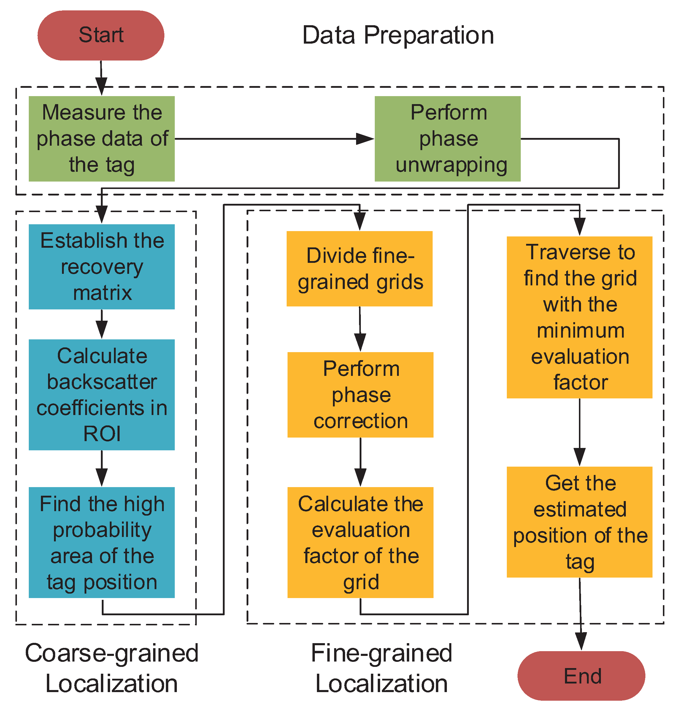
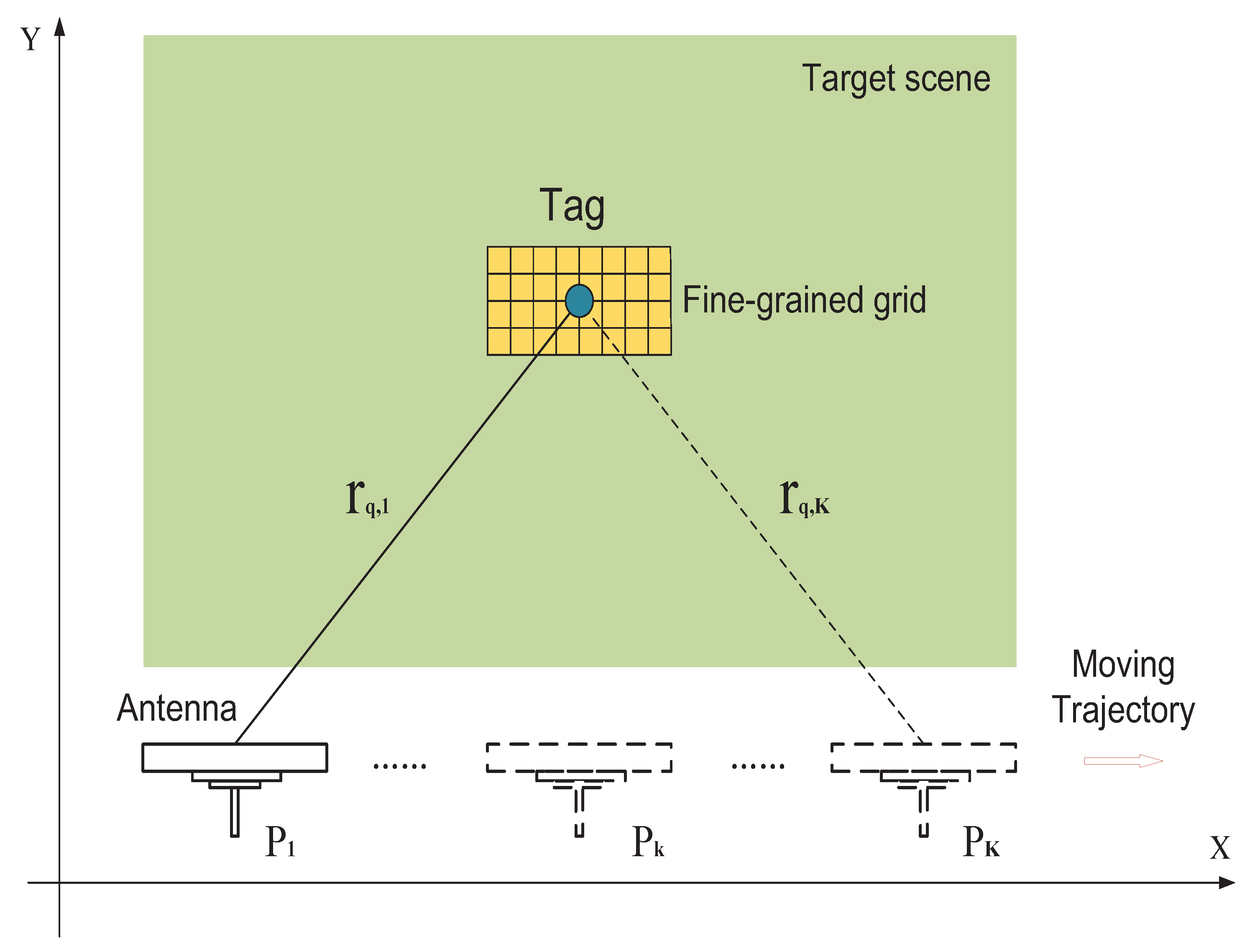
3. RF-SML Localization Methodology and Model

3.1. Basic Method of RF-SML

According to the signal feature models that are shown in Equations (1) and (2), the ideal signal that is returned by the tag can be described as the following complex exponential form

$$h=A_T{\mathrm{e}}^{{\displaystyle -j\phi }}=\sigma \beta {\mathrm{e}}^{{\displaystyle -j\left({\phi }_r+{\phi }_h\right)}},$$

(3)

where $\sigma$ is the reflection coefficient of the tag, which represents the effect of the tag backscatter on the signal. $\beta$ is a loss factor, which indicates the loss of electromagnetic waves in the space propagation path and antenna gain, etc. Because $\beta$ is susceptible to environmental influences in actual scenario that produces large errors. It is negligible and $\beta$ is set to 1 in our model.

Because RFID is a radar-derived technology, we can transfer the idea of synthetic aperture radar to localization applications. In fact, all of the objects in the target scene backscatter the electromagnetic waves emitted by the reader. Different scatterers have different reflection coefficients. Consequently, the signal received by the reader is the vector sum of the backscattered signals from the scatterers in the entire scene. In the stage of coarse-grained localization, the target scene is approximately composed of $M\times N$ uniform backscatter regions, then the reflection coefficient corresponding to each region can be written as the following vector in ${\mathbb{C}}^{MN}$

$$\mathbf{\sigma }={\left({\sigma }_{1,1},\cdots ,{\sigma }_{1,n},\cdots ,{\sigma }_{m,n},\cdots ,{\sigma }_{M,N}\right)}^T,$$

(4)

where ${\sigma }_{m,n}$ denotes the reflection coefficient of the backscatter region localized at the corresponding row and column position in the target scene. As it is known, the UHF-RFID system has special identification characteristics, because the symbol sequence of the passive tag is unique in the world. The RFID system only acquires the signal data of a single tag in an interrogation process. Under the communication mechanism, the reflection coefficient that is related to the backscatter region where the tag is localized is a non-zero value, and the reflection coefficients of the remaining regions are equal to zero.

Figure 3 shows the brief mobile localization model. In this model, the reader antenna moves along a trajectory to form a synthetic aperture. During the period, the backscattered signal of the scatterers in the target scene is received K times. In particular, the sampling position of the reader antenna is known. The subsequent localization algorithm makes use of these as priori information. During the $kth$ interrogation operation, the Euclidean distance between the antenna and the $qth$ backscatter region can be written as

$$r_{q,k}=∥{\mathbf{p}}_k-{\mathbf{p}}_q∥,$$

(5)

where ${\mathbf{p}}_k=\left[x_k,y_k\right]$ represents the sampling position of the reader antenna on the aperture, and ${\mathbf{p}}_q=\left[x_q,y_q\right]$ denotes the position of the $qth$ backscatter region. $∥·∥$ denotes the norm operator. Under ideal circumstances, the received signal that is obtained by the reader antenna at the $kth$ sampling position can be modeled as

$$\begin{array}{cc}\hfill h_k^{\prime }& ={\displaystyle \sum }_{q=1}^{MN}{\sigma }_q{e}^{{\displaystyle -j({\phi }_{r_{q,k}}+{\phi }_h)}}\hfill \\ \hfill & ={\displaystyle \sum }_{q=1}^{MN}{\sigma }_q{e}^{{\displaystyle -j(2\pi f\frac{2r_{q,k}}{c}+{\phi }_h)}},\hfill \end{array}$$

(6)

where ${\sigma }_q$ is the reflection coefficient of the $qth$ scatterer in the target scene. Subsequently, all of the received signals obtained along the trajectory can be expressed as a form of K dimensional vector

$${\mathbf{h}}^{\prime }={\left(h_1^{\prime },h_2^{\prime },\cdots ,h_k^{\prime },\cdots ,h_K^{\prime }\right)}^T.$$

(7)

As mentioned above, only the scatterer with a tag in the the target scene theoretically corresponds to the single non-zero reflection coefficient. Therefore, in order to localize the coarse-grained region containing the tag, we only need to find the position where the unique non-zero value is mapped in the reflection coefficient vector, instead of deriving the true reflection coefficient of all targets as in SAR imaging. For uniformity of the form, the actual signal data measured on the synthetic aperture is also written as a K dimensional vector $\mathbf{h}={\displaystyle {\left(h_1,h_2,\cdots ,h_k,\cdots ,h_K\right)}^T}$, in which

$$h_k=exp(-j{\phi }_k),$$

(8)

where ${\phi }_k$ is the measured phase of the reader antenna at the $kth$ sampling position. In real scenarios, the received signal should be equal to the theoretical value and related noise error. All of the measurement signals are synthesized into a matrix form, which can be calculated as

$$\mathbf{h}=\mathbf{D}\mathbf{\sigma }+\mathbf{\epsilon },$$

(9)

where $\mathbf{\epsilon }$ is the noise vector and $\mathbf{D}$ is the observation matrix. It represents the correlation between the reflection coefficients of the backscatter regions and multiple actual observations, which can be modeled as the following $K\times MN$ dimension matrix form

$$\mathbf{D}=\left(\begin{array}{cccc}{\displaystyle d_{1,1}\left(1\right)}& d_{1,2}\left(1\right)& \cdots & d_{M,N}\left(1\right)\\ d_{1,1}\left(2\right)& d_{1,2}\left(2\right)& \cdots & d_{M,N}\left(2\right)\\ ⋮& ⋮& \ddots & ⋮\\ d_{1,1}\left(K\right)& d_{1,2}\left(K\right)& \cdots & d_{M,N}\left(K\right)\end{array}\right),$$

(10)

where the elements of matrix $\mathbf{D}$ represent the ideal signal value of the $qth$ scatterer in the target scene at the $kth$ sampling position of the reader antenna, which can be expressed as

$$d_q\left(k\right)=e^{{\displaystyle -j(2\pi f\frac{2r_{q,k}}{c}+{\phi }_h)}}.$$

(11)

It can be seen that the observation matrix is related to the priori information, so the matrix $\mathbf{D}$ is known. The coarse-grained localization process is to recover the reflection coefficient vector of the target scene from the multiple measurement signals acquired by the reader antenna during the movement along the trajectory. Accordingly, the estimated value of $\mathbf{\sigma }$ is

$$\widehat{\mathbf{\sigma }}=\mathbf{Rh},$$

(12)

where $\mathbf{R}$ is the recovery matrix, Equation (12) is the inverse problem solving operation of the linear equations in Equation (9). However, due to the limitation of the real localization scenarios, the number of regional scatterers is usually greater than the number of sampling times of the reader antenna, i.e., $MN>K$. The matrix equation in Equation (9) is an ill-posed problem and the solution that satisfies the equation is not unique, but infinite. Generally, in the case, the only minimum norm solution of the matrix equation is derived from the Moore-–Penrose pseudoinverse $\mathbf{R}={\mathbf{D}}^H{\left(\mathbf{D}{\mathbf{D}}^H\right)}^{-1}$. Nevertheless, the obtained estimation value is inconsistent with the actual reflection coefficient and unable to be applied to coarse-grained localization. Inspired by the pulse compression process in the synthetic aperture imaging, the required accurate and stable reflection coefficient estimates can be given by $\mathbf{R}={\mathbf{D}}^H$, where H represents the Hermitian operator.

Because the UHF-RFID system has only one tag response in each interrogation, the non-zero reflection coefficient in $\widehat{\mathbf{\sigma }}$ is ideally unitary. In addition, the measuremental signals of several sampling positions are utilized coherently in the process of solving the reflection coefficient vector, thereby significantly reducing the influence of noise interference and multipath effects in the environment. Whereas, these environmental distortion factors still lead to multiple non-zero values in the reflection coefficient vector. Because the line-of-sight (LOS) signal normally has a higher weight in the measurement signal, the tag is localized in the backscatter region that is associated with the maximum reflection and its neighborhood. Thus, the estimation result of coarse-grained localization can be calculated as

$${\widehat{\mathbf{p}}}_{\mathbf{coa}}=\underset{q}{argmax}\left|{\widehat{\sigma }}_q\right|.$$

(13)

Accordingly, we get a high probability region of the tag position, as shown in Figure 4a, and the colors represent the normalized modulus of the reflection coefficients in the target scene. Subsequently, the region is divided into L fine-grained grids according to the required accuracy. Based on the priori information and the known position of each grid point, if the tag is localized at the $lth$ grid point, we can calculate a sequence of estimated phase values along the synthetic aperture

$${\mathbf{\gamma }}_l={\left({\theta }_{1,l},{\theta }_{2,l},\cdots ,{\theta }_{k,l},\cdots ,{\theta }_{K,l}\right)}^T.$$

(14)

And the sequence of actual phase values of the measured tag

$${\mathbf{\gamma }}_a={\left({\phi }_1,{\phi }_2,\cdots ,{\phi }_k,\cdots ,{\phi }_K\right)}^T.$$

(15)

Calculate the following cost function for any grid point in the high probability area

$$G_l=\frac{{\displaystyle {\displaystyle {\displaystyle \sum }}_{k=1}^K}\left|{\theta }_{k,l}-{\phi }_k\right|}{\left|{\displaystyle {\displaystyle {\displaystyle \sum }}_{k=1}^K}\left({\theta }_{k,l}+{\phi }_k\right)\right|},$$

(16)

where $G_l$ is an evaluation factor, which denotes the similarity between the estimated phase value sequence of grid points and the phase value sequence actually measured by the tag. Obviously, the lower the evaluation factor value is, the more similar the two phase value sequences are. If the grid point is the true position of the tag, ideally the elements in the two phase value sequences are equal, then the value of the corresponding evaluation factor is zero. Consequently, after traversing each fine-grained grid point, the final spatial estimated coordinates of the tag

$${\widehat{\mathbf{p}}}_{\mathbf{t}}=\underset{l}{argmin}\left(G_l\right).$$

(17)

3.2. Localization with Phase Correction

In this section, we propose a method to correct the phase offsets that are caused by different factors, thereby improving the performance of the RF-TRO localization algorithm.

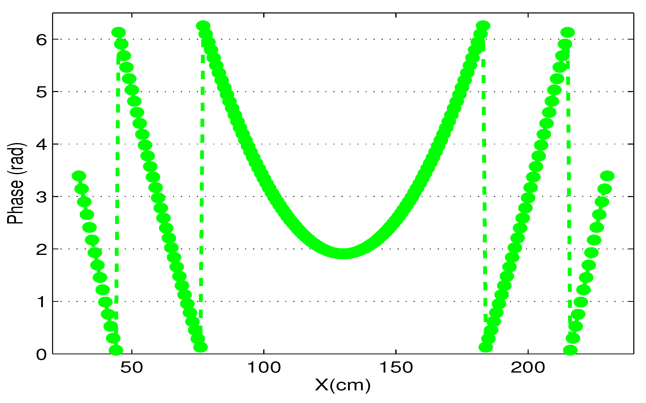
3.2.1. Correction with Phase Unwrapping

It can be seen that the measured phase value jumps in the interval $\left[0,2\pi \right]$, which does not change continuously and regularly, as shown in Figure 5. This is because the phase value reported by the reader in Equation (1) is the data obtained by taking the remainder of $2\pi$, which ignores the periodic value of electromagnetic wave propagation in space at integer wavelengths. The unknown propagation period number makes the observed phase value wrapped into $0-2\pi$. Therefore, the phase information of the received signal is unable to have an intuitive mapping relationship with the distance between the reader antenna and the tag in space, which leads to the problem of distance ambiguity. For this reason, we implement unwrapping procedures on the original measured phase value in order to eliminate the effect of phase periodic changes on localization. The phase value after unwrapping can be calculated as

$$\left\{\begin{array}{c}{\displaystyle {\eta }_1={\phi }_1}\hfill \\ \\ {\displaystyle {\eta }_{k+1}={\phi }_{k+1}-2\pi \times ⌈\frac{{\phi }_{k+1}-{\eta }_k}{2\pi }-\frac{1}{2}⌉,k=1,2,\dots ,K-1}\hfill \end{array}\right.$$

(18)

where ${\eta }_k$ is the unwrapped phase of the $kth$ measurement value, and $⌈·⌉$ represents rounding up operation. In Equation (18), the latter phase has a jump when the change between two adjacent sampled phases exceeds the threshold value $\pi$. The process of phase unwrapping is to perform the operation of increasing or decreasing $2\pi$ on the jump phase to complete the calibration. It is worth noting that the phase unwrapping method needs to meet the spatial sampling limit. This requires that the change in the path difference of the signal during the two samplings on the synthetic aperture should not be greater than a quarter of the corresponding wavelength. In this case, the absolute phase difference of consecutive sampled values is avoided to be greater than $\pi$, which prevents confusion with jumps that are caused by the periodicity of the phase. After phase unwrapping, a successive phase sequence without jumps can be restored, and the phase value is no longer limited to the period, as shown in the continuous phase result curve of the Figure 6.

3.2.2. Correction for the Phase Offset of Hardware Devices

As mentioned above, in addition to the phase part linearly related to the distance, the measured phase of the received signal also contains an unknown phase offset related to the UHF RFID hardware device. This phase offset depends on the characteristics of the reader’s antenna, transmitter and receiver circuits, deployed cables and other facility components, so it is also called device diversity. In practice, ${\phi }_h$ is affected by related parameters such as frequency and transmit power. In the existing research, the relevant calibration is usually carried out through pre-measurement. Nevertheless, a series of phase values are generally obtained by single antenna movement measurement in the scenario where the proposed method is applied. The phase offset that is introduced under the constant environment conditions can be regarded as fixed. Therefore, the difference between the measured phase values of the same tag can be leveraged to handily eliminate the unknown phase offset that is caused by this hardware diversity. The phase value at the first sampling position is regarded as a correction reference, then the evaluation factor of the fine-grained localization stage is altered into

$$G_l=\frac{{\displaystyle {\displaystyle \sum }_{k=1}^K}\left|{{\theta }^{\prime }}_{k,l}-{\eta }_k-({{\theta }^{\prime }}_{1,l}-{\eta }_1)\right|}{\left|{\displaystyle {\displaystyle \sum }_{k=1}^K}\left({{\theta }^{\prime }}_{k,l}+{\eta }_k-({{\theta }^{\prime }}_{1,l}+{\eta }_1)\right)\right|},$$

(19)

where ${{\theta }^{\prime }}_{k,l}$ represents the the unwrapped phase of ${\theta }_{k,l}$. The measurement and estimated phase values of each sampling position remove the correction reference value, which replace the original phase with the phase difference. Thus, the constant phase offset of the device is canceled.

3.2.3. Correction for the Phase Offset of the Phase Center

In many current RFID-based localization models, the phase center of the reader antenna is generally reduced to a theoretical fixed point. This is because it assumes that the antenna radiated waves form an ideal spherical surface. However, the radiation wave surface of the antenna actually applied has irregular fluctuations, and this deviation from the ideal phase center will introduce a corresponding phase offset. Moreover, the actual phase center varies with the direction of arrival of the received signal. Different sampling positions have different reception angles for the backscattered signal under the circumstance of the moving reader antenna, which results in inconsistent phase offsets, as can be seen in the Figure 7. At present, there have been researches on methods for measuring the real phase center of antennas. However, the required experimental conditions and equipment are complicated, these measurements could not be practically applied in SAR-based localization. In real scenarios, the mobile reader antenna works at a fixed frequency. Accordingly, we can measure the phase offset that is associated with AoA by advance experiments. The difference between the ideal phase and the measured phase is the sum of phase offset caused by the fixed device and the phase offset caused by the angle. Therefore, the specific phase offsets at different angles are retrieved from the curve fitted by the phase difference data.

In the stage of fine-grained localization, the angle of each grid relative to each sampling position is first calculated by priori knowledge, then the phase offset value of the angle is corrected for phase compensation, thereby achieving more accurate localization performance. Thus, we change the evaluation factor as

$$G_l=\frac{{\displaystyle {\displaystyle \sum }_{k=1}^K}\left|{{\theta }^{\prime }}_{k,l}+{\beta }_{k,l}-{\eta }_k-({{\theta }^{\prime }}_{1,l}+{\beta }_{1,l}-{\eta }_1)\right|}{\left|{\displaystyle {\displaystyle \sum }_{k=1}^K}\left({{\theta }^{\prime }}_{k,l}+{\beta }_{k,l}+{\eta }_k-({{\theta }^{\prime }}_{1,l}+{\beta }_{1,l}+{\eta }_1)\right)\right|},$$

(20)

where ${\beta }_{k,l}$ is the phase offset value related to the angle of the reader antenna at the $kth$ sampling position relative to the $lth$ grid point position. It can be seen from Figure 4b,c that the estimated position after phase correction is closer to the ground truth. Additionally, the colors in figures indicate the normalized evaluation factor corresponding to each grid point in the high probability region of the tag position.

4. Measurement and Performance Analysis

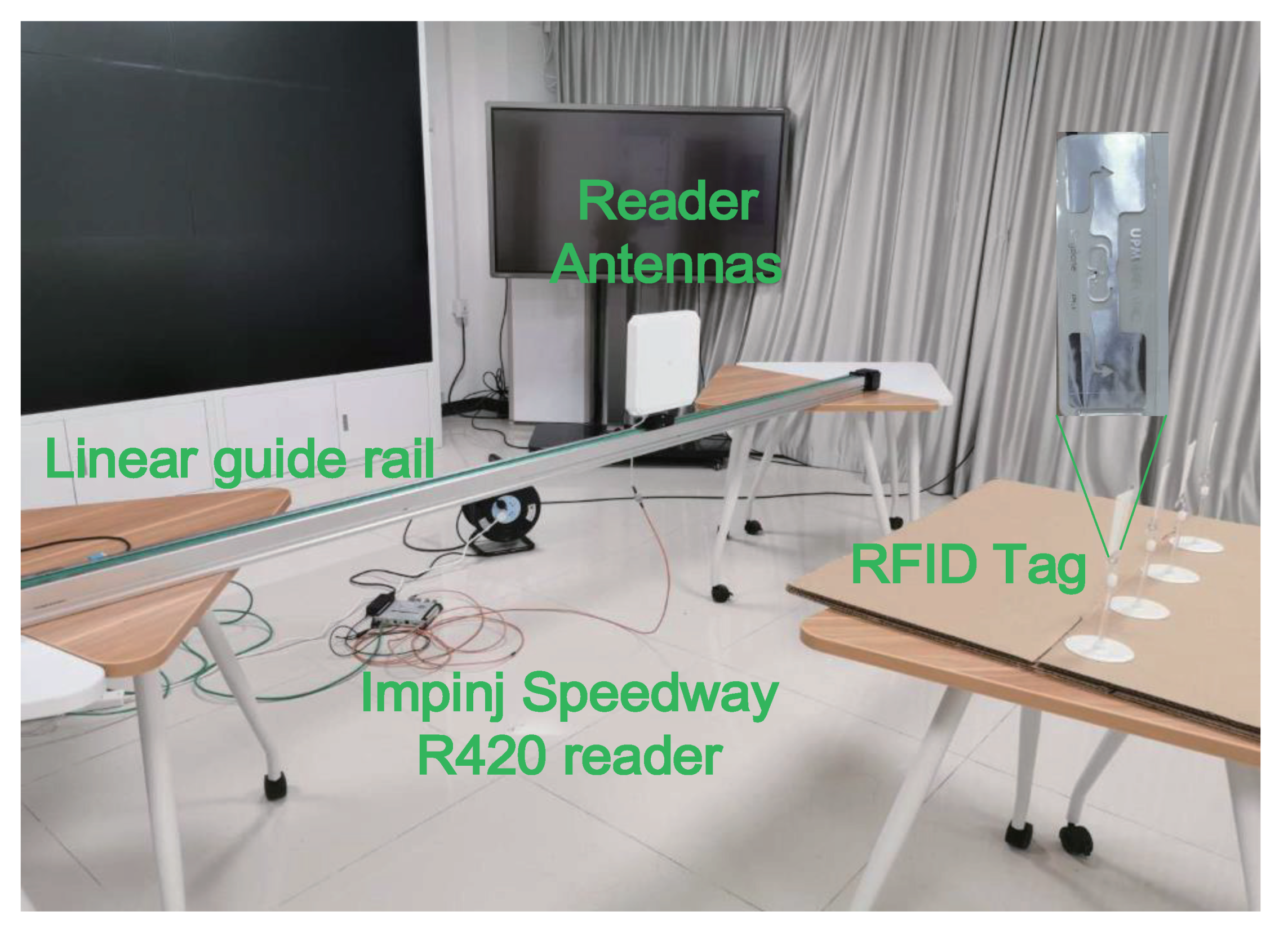
4.1. Experimental Setup

A series of experiments are performed in the environment within the laboratory to evaluate the performance of the proposed method and the influence of related factors on it. The experimental scene is shown in Figure 8, which includes a Laird S9028PCL antenna, an Impinj Speedway R420 reader, a Fuyu FBL-60 linear guide, and several UPM RAFLATAC DogBone tags. The facilities used are existing commercial products without any arbitrary modification. The RF-SML algorithm runs on a Lenovo personal laptop equipped with 8 GB memory and a Inter (R) Core (TM) i5-8300H CPU at 2.30 GHz. The applied operating system is 64-bit Windows 10 version. The antenna is left-handed circularly polarized with a size of ${10.2}^{″}\times {10.2}^{″}\times {1.32}^{″}$ and it has a 9 dBiC gain. The reader adopted supports the EPCglobal Gen2 protocol, whose frequency band is 920.625–924.375 MHz and maximum allowable transmit power is 32.5 dBm. The tag is passive linear polarized, which is deployed in a location area of 1 m × 1.2 m. The actual position coordinates are observed by the BOSCH GLM 500 laser rangefinder with a maximum error of 1.5 mm. The antenna is installed on the platform of the linear guide rail to move in the direction of the x coordinate axis. During this period, the reader continues to interrogate the tags. Accordingly, the sampling position of the reader antenna is accurately obtained from the rail controller with a maximum error of 0.04 mm.

4.2. Analysis of Affecting Factor Parameters

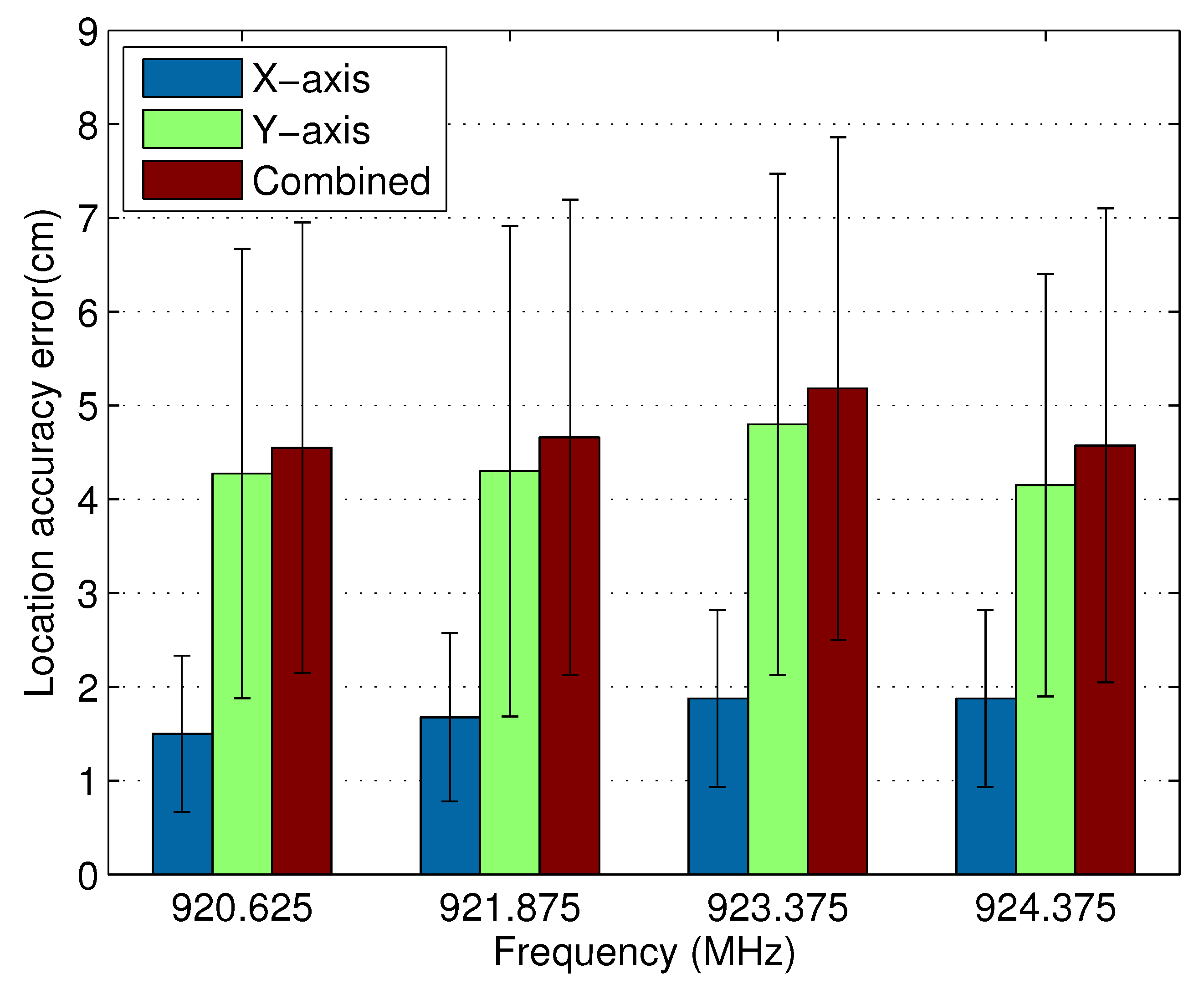
4.2.1. The Impact of Carrier Frequency

First, we analyze the effect of the change in carrier frequency on the localization accuracy. In the experiment, four channels of 920.625 MHz, 921.875 MHz, 923.375 MHz, and 924.375 MHz are selected for testing. The frequency is fixed during the localization process, and the aperture length formed by the movement of the reader antenna is set as 2 m. The spatial interval of two consecutive samples of the reader is set as 0.01 m. A total of 160 measurement results are obtained. Figure 9 shows the average localization accuracy of RF-SML in x-axis, y-axis, and combined dimension when the sampling frequencies are these four channels. The localization errors of the x and y coordinate axes can be expressed as $x\_error=\left|x-\widehat{x}\right|$ and $y\_error=\left|y-\widehat{y}\right|$, respectively. The localization error of the combined result is defined as the Euclidean distance between the actual tag position ${\mathbf{p}}_{\mathbf{t}}$ and the estimated tag position ${\widehat{\mathbf{p}}}_{\mathbf{t}}$, whose calculation formula is $combined\_error=∥{\mathbf{p}}_{\mathbf{t}}-{\widehat{\mathbf{p}}}_{\mathbf{t}}∥$. It can be seen that different frequencies have little effect on the localization result error. This is because the 3.75 MHz bandwidth of UHF RFID is relatively narrow, and the corresponding wavelength has a little variation. Therefore, the localization accuracy changes little with the carrier frequency. When compared with the x-axis, the localization error of the y-axis increases more greatly. Additionally, the localization accuracy of the x-axis is always higher than the y-axis. This is because the synthetic aperture that is formed by the movement of the reader antenna is along the x-axis direction. If the antenna is subjected to a two-dimensional movement mode, it can achieve better positioning accuracy in the y-axis direction [22].

4.2.2. The Impact of Sampling Interval

We observe the effect of the change in the sampling interval (the distance between the position of the reader antenna for two consecutive phase measurements) on the localization accuracy. In the experiment the frequency is fixed at 920.625 MHz, and the aperture length is constantly set as 2 m. In the meantime the sampling positions of the reader antenna are evenly distributed, so different spatial sampling intervals would result in different measurement phase numbers. We set the sampling interval from 1 cm to 8 cm and obtain 200 test results. Figure 10 shows the corresponding average localization accuracy of x-axis, y-axis, and combined position results. It can be seen that the localization result error also decreases as the sampling interval decreases. This is because the smaller sampling interval gets more measured phase values. However, even at the maximum sampling interval, RF-SML still has great localization performance. When the sampling interval is greater than 8 cm, the phase unwrapping is likely to fail due to its exceeding the spatial sampling limit. It is worth mentioning that the experiment is set to evenly spaced sampling in order to accurately study the influence of parameters. In practical applications, unevenly spaced sampling is usually caused by the environmental factors. If the sampling position of the antenna can be obtained in this case, the localization method in the paper is also available in this situation.

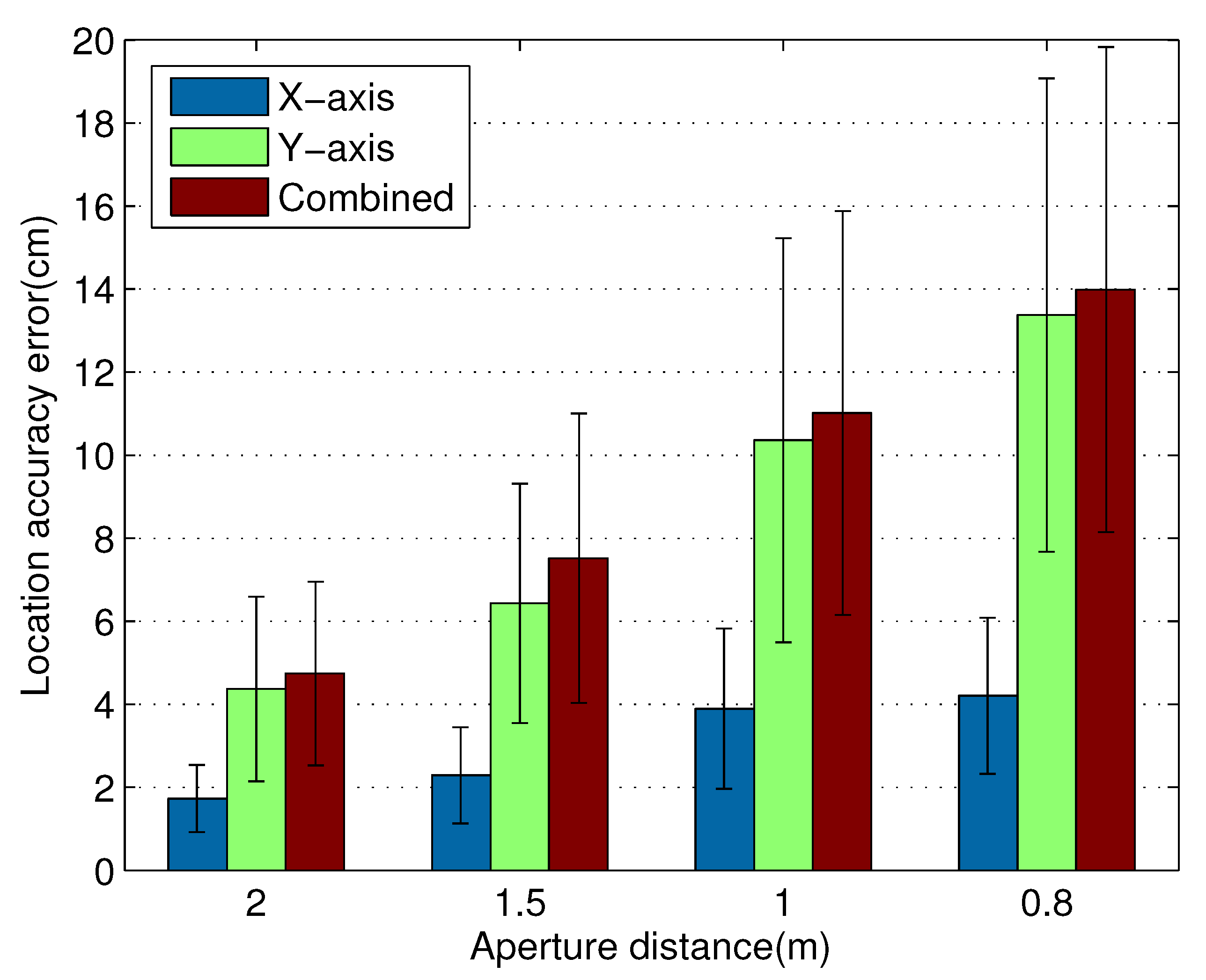
4.2.3. The Impact of Reader Antenna Movement Distance

We investigate the influence of different aperture lengths (the total distance of reader antenna motion) on the localization performance in the experiment. The frequency is set as 920.625 MHz, and the sampling interval of the reader antenna is fixed at 0.01 m. Accordingly, larger aperture lengths also have more measured phase values. 160 sets of test results are obtained As shown in Figure 11, we compare the average localization accuracy of the x-axis, y-axis and the combined position when the aperture lengths are 0.8 m, 1 m, 1.5 m, and 2 m. The experimental results show that the localization error increases significantly with the decrease of the aperture length. It is worth mentioning that the effect of the aperture length on the localization error is more obvious than the sampling interval, although both cause changes in the number of measurement phases. This is because the smaller sampling interval only reduces the sensitivity of the system to small measurement fluctuations of the phase, while the larger aperture length increases the discrimination of the phase data itself and, thus, improves the robustness of the system.

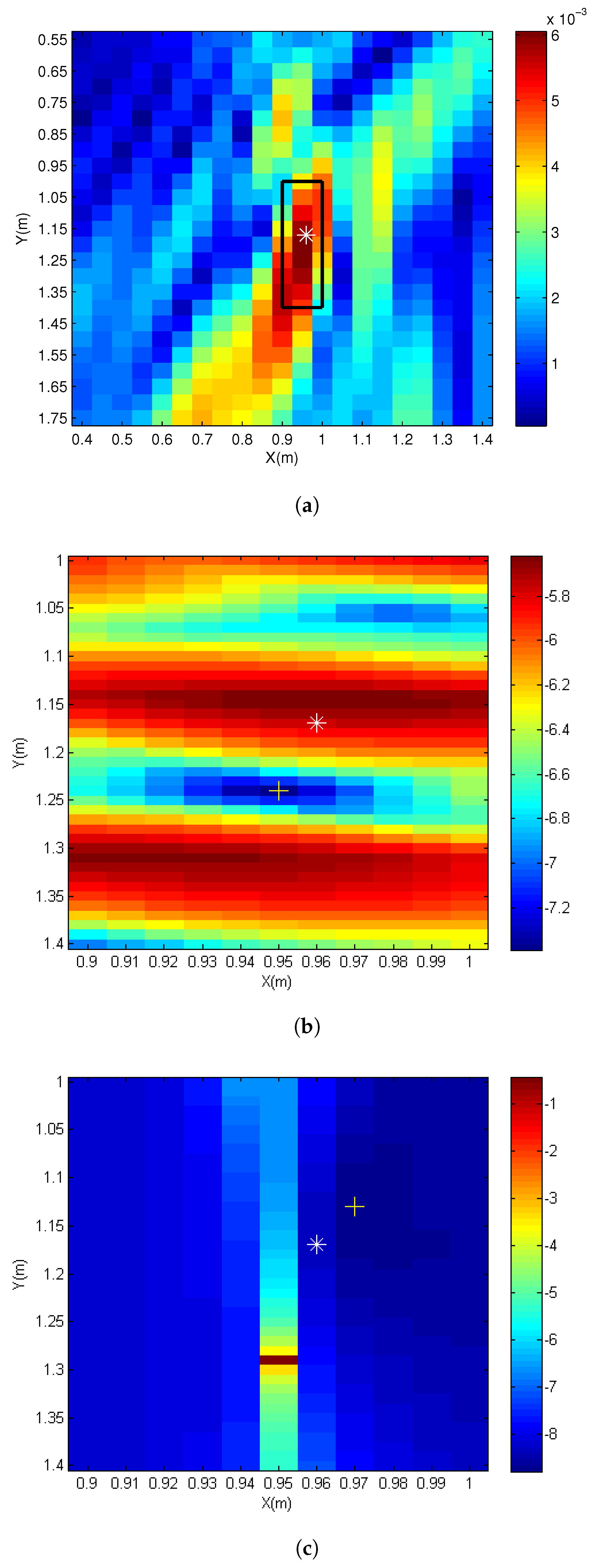
4.3. Performance of RF-SML

4.3.1. Localization Accuracy

We repeat the experiment and obtain 240 test results, and the cumulative distribution function (CDF) curve of the localization errors on the proposed method is shown in the Figure 12. The mean localization accuracy of RF-SML in the x-axis, y-axis and combined position results are 1.93 cm, 5.96 cm, and 6.47 cm, and the standard deviations are 1.04 cm, 2.92 cm, and 2.82 cm, respectively. We compared the localization accuracy of RF-SML with two current typical SAR RFID methods: SARFID [22,27] and Tagoram [26]. We use the same equipment and data to implement these methods. Figure 13 shows the results. The mean localization accuracy of SARFID are 2.98 cm, 8.18 cm, and 9.50 cm, and the standard deviations are 1.45 cm, 4.23 cm, and 8.78 cm. The mean accuracy of Tagoram are 2.38 cm, 7.85 cm, and 8.30 cm, and the standard deviation are 1.22 cm, 6.87 cm, and 7.46 cm. The results show that the localization performance of RF-oto is better than SARFID and Tagoram. This is because the phase correction method can reduce the negative effects of phase errors, which is helpful to improve the positioning accuracy, as described above.

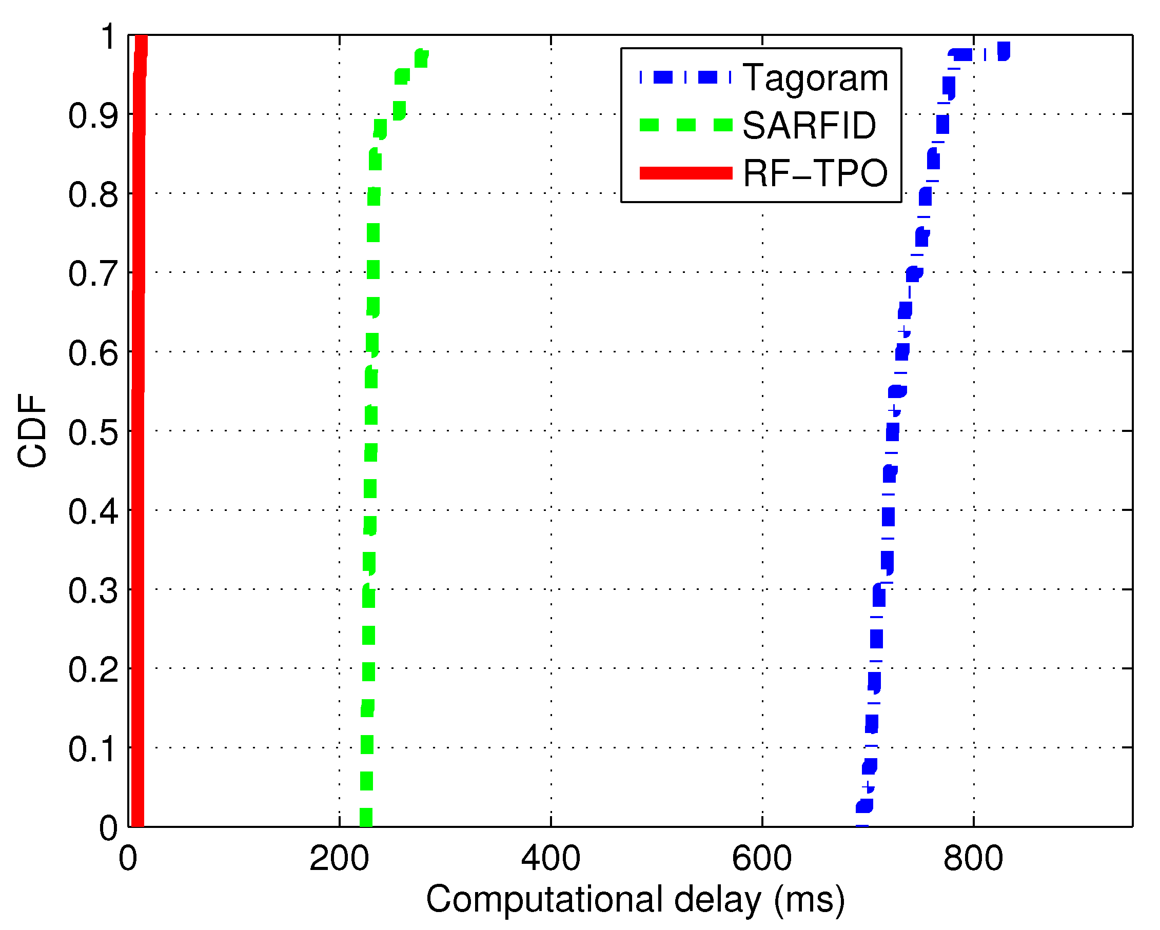
4.3.2. Computational Latency

The more obvious advantage of RF-SML is that it reduces the amount of calculation in the localization process. Figure 14 shows the CDF curves of the above three methods for computational time. The average computation time of SARFID and Tagoram is 233.55 ms and 708.86 ms. The RF-SML is 9.68 ms, whose calculation efficiency is 24.1× and 73.2× higher than SARFID and Tagoram, respectively. It can be seen that the proposed method reduces the computational cost by up to about 98.6% when compared with other methods in the two-dimensional (2D) search space, thereby reducing the localization latency and achieving the computational time of the millisecond level. This is because RF-SML introduces the idea of multi-granularity based on the reflection coefficient model, which improves real-time performance. The corresponding improvement will be more obvious in the extension to 3D search space because of the sharply increased computation. It is foreseeable that the method is able to execute rapid localization of large-scale items with mobile devices, which has great practical value in the environment of intelligent manufacturing and warehousing.

5. Conclusions

This paper proposes and implements a novel fast and accurate localization method that is based on UHF RFID technology, termed RF-SML. Through specific theoretical analysis, RF-SML makes full use of priori knowledge in the coarse-grained stage to model the localization problem as a regional reflection coefficient reconstruction problem and find the high-probability region where the tag position is. Subsequently, in the fine-grained stage, the evaluation factor is calculated by traversing the grid to achieve the final localization. While the multi-granularity idea reduces the computational burden, we improve the localization accuracy by calibrating the phase offsets that are caused by the hardware device and phase center. Experimental verification is carried out with COTS RFID equipment. Additionally, the results show that the method reduces 98.6% of the calculation time delay and has a comparative accurate localization performance compared with the typical hologram methods. In addition, the aperture length and sampling interval both affect the localization accuracy. The lower localization error can be obtained with smaller sampling intervals or longer aperture lengths. Our future work will further study multipath effects, and achieve better positioning performance by multipath interference suppression.

References

1. Kuutti, S.; Fallah, S.; Katsaros, K.; Dianati, M.; Mccullough, F.; Mouzakitis, A. A Survey of the State-of-the-Art Localization Techniques and Their Potentials for Autonomous Vehicle Applications. IEEE Internet Things J. 2018, 5, 829–846. [Google Scholar] [CrossRef]
2. Park, J.; Kim, Y.J.; Lee, B.K. Passive Radio-Frequency Identification Tag-Based Indoor Localization in Multi-Stacking Racks for Warehousing. Appl. Sci. 2020, 10, 3623. [Google Scholar] [CrossRef]
3. Ma, L.; Liu, M.; Wang, H.; Yang, Y.; Wang, N.; Zhang, Y. WallSense: Device-Free Indoor Localization Using Wall-Mounted UHF RFID Tags. Sensors 2018, 19, 68. [Google Scholar] [CrossRef] [PubMed] [Green Version]
4. Ma, Y.; Wang, B.; Gao, X.; Ning, W. The Gray Analysis and Machine Learning for Device-Free Multitarget Localization in Passive UHF RFID Environments. IEEE Trans. Ind. Inform. 2020, 16, 802–813. [Google Scholar] [CrossRef]
5. Ma, Y.; Song, L.; Zhao, Y.; Liu, K. A tight outer bound of the degrees of freedom for the MIMO interference channel with the delayed CSIT and partial local feedback. J. Frankl. Inst. 2015, 352, 291–310. [Google Scholar] [CrossRef]
6. Ma, Y.; Tian, C.; Jiang, Y. A Multitag Cooperative Localization Algorithm Based on Weighted Multidimensional Scaling for Passive UHF RFID. IEEE Internet Things J. 2019, 6, 6548–6555. [Google Scholar] [CrossRef]
7. El-Absi, M.; Zheng, F.; Abuelhaija, A.; Abbas, A.H.; Kaiser, T. Indoor Large-Scale MIMO-Based RSSI Localization with Low-Complexity RFID Infrastructure. Sensors 2020, 20, 3933. [Google Scholar] [CrossRef] [PubMed]
8. Wang, T.; Xiong, H.; Ding, H.; Zheng, L. TDOA-Based Joint Synchronization and Localization Algorithm for Asynchronous Wireless Sensor Networks. IEEE Trans. Commun. 2020, 68, 3107–3124. [Google Scholar] [CrossRef]
9. Geng, C.; Yuan, X.; Huang, H. Exploiting Channel Correlations for NLOS ToA Localization with Multivariate Gaussian Mixture Models. IEEE Wirel. Commun. Lett. 2020, 9, 70–73. [Google Scholar] [CrossRef]
10. Scherhäufl, M.; Pichler, M.; Stelzer, A. Robust localization of passive UHF RFID tag arrays based on phase-difference-of-arrival evaluation. In Proceedings of the IEEE Topical Conference on Wireless Sensors and Sensor Networks (WiSNet), San Diego, CA, USA, 25–28 January 2015; pp. 47–49. [Google Scholar]
11. Zheng, Y.; Sheng, M.; Liu, J.; Li, J. Exploiting AoA Estimation Accuracy for Indoor Localization: A Weighted AoA-Based Approach. IEEE Wirel. Commun. Lett. 2019, 8, 65–68. [Google Scholar] [CrossRef]
12. Wang, Y.; Ho, K.C. Unified Near-Field and Far-Field Localization for AOA and Hybrid AOA-TDOA Positionings. IEEE Trans. Wireless Commun. 2018, 17, 1242–1254. [Google Scholar] [CrossRef]
13. Wu, X.; Deng, F.; Chen, Z. RFID 3D-LANDMARC Localization Algorithm Based on Quantum Particle Swarm Optimization. Electronics 2018, 7, 19. [Google Scholar]
14. Shi, W.; Du, J.; Cao, X.; Yu, Y.; Cao, Y.; Yan, S.; Ni, C. IKULDAS: An Improved kNN-Based UHF RFID Indoor Localization Algorithm for Directional Radiation Scenario. Sensors 2019, 19, 968. [Google Scholar] [CrossRef] [PubMed] [Green Version]
15. Liu, M.; Ma, L.; Wang, N.; Zhang, Y.; Yang, Y.; Wang, H. Passive Multiple Target Indoor Localization Based on Joint Interference Cancellation in an RFID System. Sensors 2019, 8, 426. [Google Scholar] [CrossRef] [Green Version]
16. Zafari, F.; Gkelias, A.; Leung, K.K. A Survey of Indoor Localization Systems and Technologies. IEEE Commun. Surv. Tutor. 2019, 21, 2568–2599. [Google Scholar] [CrossRef] [Green Version]
17. Zhang, H.; Zhang, Z.; Gao, N.; Xiao, Y.; Meng, Z.; Li, Z. Cost-Effective Wearable Indoor Localization and Motion Analysis via the Integration of UWB and IMU. Sensors 2020, 20, 344. [Google Scholar] [CrossRef] [Green Version]
18. Ma, Y.; Gao, Z.; Zhao, Y. RFID Indoor Localization Techniques. In Positioning and Navigation in Complex Environments; Yu, K., Ed.; IGI Global: Hershey, PA, USA, 2018; pp. 142–192. [Google Scholar]
19. Mulloni, V.; Donelli, M. Chipless RFID Sensors for the Internet of Things: Challenges and Opportunities. Sensors 2020, 20, 2135. [Google Scholar] [CrossRef] [Green Version]
20. Fu, X.; Pedross-Engel, A.; Arnitz, D.; Watts, C.M.; Sharma, A.; Reynolds, M.S. Simultaneous Imaging, Sensor Tag Localization, and Backscatter Uplink via Synthetic Aperture Radar. IEEE Trans. Microw. Theory Tech. 2018, 66, 1570–1578. [Google Scholar] [CrossRef]
21. Miesen, R.; Kirsch, F.; Vossiek, M. UHF RFID Localization Based on Synthetic Apertures. IEEE Trans. Autom. Sci. Eng. 2013, 10, 807–815. [Google Scholar] [CrossRef]
22. Buffi, A.; Motroni, A.; Nepa, P.; Tellini, B.; Cioni, R. A SAR-Based Measurement Method for Passive-Tag Positioning with a Flying UHF-RFID Reader. IEEE Trans. Instrum. Meas. 2019, 68, 845–853. [Google Scholar] [CrossRef]
23. Shangguan, L.; Jamieson, K. The Design and Implementation of a Mobile RFID Tag Sorting Robot. In Proceedings of the 14th Annual International Conference on Mobile Systems, Applications, and Services (MOBISYS), Singapore, 26–30 June 2016; pp. 31–42. [Google Scholar]
24. Parr, A.; Miesen, R.; Vossiek, M. Inverse SAR approach for localization of moving RFID tags. In Proceedings of the IEEE International Conference on RFID (RFID), Orlando, FL, USA, 30 April–2 May 2013; pp. 104–109. [Google Scholar]
25. Scherhäufl, M.; Pichler, M.; Stelzer, A. Localization of passive UHF RFID tags based on inverse synthetic apertures. In Proceedings of the IEEE International Conference on RFID (RFID), Orlando, FL, USA, 8–10 April 2014; pp. 82–88. [Google Scholar]
26. Yang, L.; Chen, Y.; Li, X.; Xiao, C.; Li, M.; Liu, Y. Tagoram: Real-Time Tracking of Mobile RFID Tags to High Precision Using COTS Devices. In Proceedings of the 20th Annual International Conference on Mobile Computing and Networking (MOBICOM), Maui, HI, USA, 7–11 September 2014; pp. 237–248. [Google Scholar]
27. Buffi, A.; Nepa, P.; Lombardini, F. A Phase-Based Technique for Localization of UHF-RFID Tags Moving on a Conveyor Belt: Performance Analysis and Test-Case Measurements. IEEE Sens. J. 2015, 15, 387–396. [Google Scholar] [CrossRef]
28. Duan, C.; Yang, L.; Lin, Q.; Liu, Y. Tagspin: High Accuracy Spatial Calibration of RFID Antennas via Spinning Tags. IEEE Trans. Mob. Comput. 2018, 17, 2438–2451. [Google Scholar] [CrossRef]
29. Shen, L.; Zhang, Q.; Pang, J.; Xu, H.; Xue, D. ANTspin: Efficient Absolute Localization Method of RFID Tags via Spinning Antenna. Sensors 2019, 19, 2194. [Google Scholar] [CrossRef] [PubMed] [Green Version]
30. Wang, J.; Katabi, D. Dude, Where’s My Card? RFID Positioning That Works with Multipath and Non-Line of Sight. ACM SIGCOMM Comput. Commun. Rev. 2013, 43, 51–62. [Google Scholar] [CrossRef]
31. Bu, Y.; Xie, L.; Gong, Y.; Liu, J.; He, B.; Cao, J.; Ye, B.; Lu, S. RF-3DScan: RFID-based 3D Reconstruction on Tagged Packages. IEEE Trans. Mob. Comput. 2019. [Google Scholar] [CrossRef]
32. Fu, Y.; Wang, C.; Liu, R.; Liang, G.; Zhang, H.; Ur Rehman, S. Moving Object Localization Based on UHF RFID Phase and Laser Clustering. Sensors 2018, 18, 825. [Google Scholar] [CrossRef] [Green Version]
33. Rehman, S.U.; Liu, R.; Zhang, H.; Liang, G.; Qayoom, A. Localization of Moving Objects Based on RFID Tag Array and Laser Ranging Information. Electronics 2019, 8, 887. [Google Scholar] [CrossRef] [Green Version]
34. Zhao, R.; Zhang, Q.; Li, D.; Chen, H.; Wang, D. A novel accurate synthetic aperture RFID localization method with high radial accuracy. In Proceedings of the IEEE 18th International Symposium on a World of Wireless, Mobile and Multimedia Networks (WoWMoM), Macau, China, 12–15 June 2017; pp. 1–9. [Google Scholar]
35. Parr, A.; Miesen, R.; Vossiek, M. Comparison of Phase-Based 3D Near-Field Source Localization Techniques for UHF RFID. Sensors 2016, 16, 978. [Google Scholar] [CrossRef] [Green Version]
36. Buffi, A.; Pino, M.R.; Nepa, P. Experimental validation of a SAR-Based RFID localization technique exploiting an automated handling system. IEEE Antennas Wirel. Propag. Lett. 2017, 16, 2795–2798. [Google Scholar] [CrossRef]
37. Ma, Y.; Liu, H.; Zhang, Y.; Jiang, Y. The Influence of the Non-ideal Phase Offset on SAR-Based Localization in Passive UHF RFID. IEEE Trans. Antennas Propag. 2020. [Google Scholar] [CrossRef]
38. Qiu, L.; Huang, Z.; Wirström, N.; Voigt, T. 3DinSAR: Object 3D localization for indoor RFID applications. In Proceedings of the IEEE International Conference on RFID (RFID), Orlando, FL, USA, 3–5 May 2016; pp. 1–8. [Google Scholar]
39. Nikitin, P.V.; Martinez, R.; Ramamurthy, S.; Leland, H.; Spiess, G.; Rao, K.V.S. Phase based spatial identification of UHF RFID tags. In Proceedings of the IEEE International Conference on RFID (RFID), Orlando, FL, USA, 14–16 April 2010; pp. 102–109. [Google Scholar]
Figure 1. The flow chart for RF-SML system. The algorithm consists of three parts: the data preparation, the coarse-grained localization, and the fine-grained localization.
Electronics 09 01447 g001
Figure 2. Radio frequency identification (RFID) signal propagation model.
Electronics 09 01447 g002
Figure 3. RF-SML localization model (the reader antenna moves along the x-coordinate axis).
Electronics 09 01447 g003
Figure 4. Localization results of the RF-SML algorithm. (a) The coarse-grained localization. (b) The fine-grained localization without phase correction. (c) The fine-grained localization with phase correction. The black outline indicates the high probability region of the tag. The white asterisk and the yellow cross represent the estimated position and the ground truth, respectively.
Electronics 09 01447 g004
Figure 5. The wrapped phase curve.
Electronics 09 01447 g005
Figure 6. The unwrapped phase curve.
Electronics 09 01447 g006
Figure 7. Antenna phase center offset related to AOA.
Electronics 09 01447 g007
Figure 8. Experimental environment and equipment.
Electronics 09 01447 g008
Figure 9. Localization accuracy error comparison with regard to the frequency. The bars represent the average localization accuracy errors in x-axis, y-axis and combined dimension, respectively. Additionally, the whiskers represent the standard deviations of the corresponding localization accuracy errors.
Electronics 09 01447 g009
Figure 10. Localization accuracy error comparison with regard to the sampling interval. The bars represent the average localization accuracy errors in x-axis, y-axis and combined dimension, respectively. And the whiskers represent the standard deviations of the corresponding localization accuracy errors.
Electronics 09 01447 g010
Figure 11. Localization accuracy error comparison with regard to the aperture distance. The bars represent the average localization accuracy errors in x-axis, y-axis and combined dimension, respectively. Additionally, the whiskers represent the standard deviations of the corresponding localization accuracy errors.
Electronics 09 01447 g011
Figure 12. Cumulative distribution function (CDF) of RF-SML localization accuracy.
Electronics 09 01447 g012
Figure 13. Localization accuracy error comparison among different methods. The bars represent the average localization accuracy errors in x-axis, y-axis, and combined dimension, respectively. Additionally, the whiskers represent the standard deviations of the corresponding localization accuracy errors.
Electronics 09 01447 g013
Figure 14. Computational delay comparison among different methods
Electronics 09 01447 g014