Approaching the Optimal Solution of the Maximal α-quasi-clique Local Community Problem

Abstract

Complex networks analysis (CNA) has attracted so much attention in the last few years. An interesting task in CNA complex network analysis is community detection. In this paper, we focus on Local Community Detection, which is the problem of detecting the community of a given node of interest in the whole network. Moreover, we study the problem of finding local communities of high density, known as α-quasi-cliques in graph theory (for high values of $\alpha$ in the interval ]0,1[). Unfortunately, the higher $\alpha$ is, the smaller the communities become. This led to the maximal α-quasi-clique community of a given node problem, which is, the problem of finding local communities that are $\alpha$-quasi-cliques of maximal size. This problem is NP-hard, then, to approach the optimal solution, some heuristics exist. When $\alpha$ is high (>0.5) the diameter of a maximal $\alpha$-quasi-clique is at most 2. Based on this property, we propose an algorithm to calculate an upper bound to approach the optimal solution. We evaluate our method in real networks and conclude that, in most cases, the bound is very accurate. Furthermore, for a real small network, the optimal value is exactly achieved in more than 80% of cases.

1. Introduction

Since the beginning of 2000s, the study of complex networks (network-based representations of complex systems) has become an active area of research. Inspired largely by the empirical study of real-world networks, such as computer networks, technological networks, brain networks, and social networks. Researchers from biology to physics, from economics to mathematics, and from computer science to sociology, are increasingly involved with the collection, modeling, and analysis of network-indexed data.

Concretely, a network can be seen as a set of entities, called vertices or nodes, which are connected by links, also called edges. Real-world complex networks often exhibit community structures (see [1]). Roughly speaking, communities are subgroups of nodes in the network that are densely connected within them, whereas sparsely connected with the rest of the network. Community detection is a tool useful for analyzing the structure of the network, visualization, or prediction of various phenomena, like the diffusion of information for social recommendation.

In some situations, the network can be so large that we do not have access to information concerning the entire network. Furthermore, one can be only interested in the community of some particular nodes in the network. The detection of the community of a given node of interest is called local community detection problem. In contrast with most community detection algorithms that decompose the entire network in groups. Moreover, detecting the local communities of specific nodes may be very important for applications dealing with huge networks, when iterating through all nodes would be impractical.

There is not a unanimous definition of community, however, this latter is usually referred to as a set of nodes densely connected, which implies strong relationships within the community. From this, one can easily deduce that in the ideal case, a community is a complete clique (a set of nodes where every two distinct nodes are connected to each other). However, the size of a clique is limited by the degree of its nodes and for most real complex networks, the degree distribution follows a power law (only a few nodes have many connections). As a result, the existing cliques can be very small or even trivial, such as pair of nodes or triangles. This led to the relaxation of the concept of a complete clique to an almost complete subgraph, also called quasi-clique. Hence, this article deals with the problem of finding quasi-cliques of maximal size (this is a well-known problem in graph theory. The interested reader can see [2,3,4,5]). More precisely, a quasi-clique is related to the concept of an $\alpha$-quasi-clique (for a given $\alpha$, such that $0<\alpha <1$). An $\alpha$-quasi-clique is a group of nodes where each member is connected to more than a proportion $\alpha$ of the other nodes. This guarantees that the resulting communities will have a density greater than $\alpha$ (if $\alpha =1$ we have a complete clique. In contrast, most commonly used community detection methods do not ensure anything about the density of the resulting communities, such as the Newman-Girvan modularity [6] due to its resolution limit [7].

For all of the reasons previously mentioned, we treat the problem of finding local communities of type $\alpha$-quasi-clique of maximal size and we call it "The maximal $\alpha$-quasi-clique local community problem". This problem is NP-complete (see [8,9]), then, some heuristics were proposed [10,11]). Although heuristics allow to approach the optimal solution in a reasonable amount of time, they do not guarantee optimality. Therefore, the main contribution of this paper is an upper bound for the optimal solution. This latter can be useful to measure how close the obtained solution by an heuristic is to the optimal one, thus, it is very useful to evaluate the performance of any heuristic. An upper bound has already been proposed in [12]. In this paper, we propose an improved version taking into account that for $\alpha >0.5$ the diameter of an $\alpha$-quasi-clique is, at most, 2 (see [11]). This property implies mining only the first and second neighborhood of the starting node which simplifies considerably the task in terms of time and space. As we do not need to have any knowledge about the graph structure beyond the second neighborhood. Furthermore, we have particular interest in detecting $\alpha$-quasi-cliques for high values of $\alpha$. The calculation of the proposed bound has two parts: the calculation of a bound per se for the starting node and its neighborhood as well as an improvement part. Another contribution of this paper is a graphical solution or visualization of the calculation of the upper bound. This graphical scheme allows to highlight that the main calculation of the bound can be reduced to a binary search algorithm, which considerably reduces the execution time in comparison to the previous version described in [12].

This paper is organized, as follows: Section 2 presents the main definitions and notations. Next, we discuss the proposed upper bound in Section 3. Subsequently, Section 4 presents experimental results with real networks as well as comparison with the existing version of the bound. Finally, Section 5 draws some conclusions and perspectives.

2. Main Definitions and Notations

A graph $G=(V,E),$ is defined by a set of vertices or nodes, denoted V, and a the set of edges or links, denoted E, formed by pairs of vertices. To simplify, we only consider undirected graphs, where the edges are not oriented. The neighborhood $\Gamma \left(u\right)$ of a node u is the set of nodes v, such that $(u,v)\in E$. The degree of a node u, denoted $d\left(u\right)$, is the number of its neighbors, i.e., $d\left(u\right)=|\Gamma (u\left)\right|$. Subsequently, the definition of an $\alpha$-quasi-clique is given in Definition 1.

Definition 1 ($\alpha$-quasi-clique)Given an undirected graph $G(V,E)$ and a parameter α with $0<\alpha <1$, an α-quasi-clique is a subgraph induced by a subset of the node set $C\subseteq V$ if the following condition holds:

$$|\Gamma (n)\cap C|>\alpha \left(\right|C|-1),\forall n\in C.$$

(1)

where the symbols $\left|S\right|$ denotes the cardinality of the set S.

Equation (1) implies that each node in the quasi-clique C must be connected to more than a proportion $\alpha$ of the other nodes. Notice that for $\alpha =1$ an $\alpha$-quasi-clique is a complete clique. Subsequently, when $\alpha$ is high, the resulting communities are robust, contain strongly connected nodes and have an edge-density greater than $\alpha$ (see [11] for the proof). Hereafter, the Equation (1) will be referred to as the rule of an $\alpha$-quasi-clique. This rule constitutes a lower bound on the minimal internal connections of each node. In the scientific literature, one can find other definitions of the so-called $\alpha$-quasi-clique. The most common variant is a relaxation of Definition 1 as it just constraints the global density of the quasi-clique to be at least $\alpha$ (see for instance [13,14,15,16]). Other variants much closer to Definition 1 are considered by [17,18]. However, these latter allow for the equality in Equation (1), which implies that a node might have as many connections as non-connections in the community. The advantage of the Definition 1 is that for any $\alpha \ge 0.5$, it constrains at least the absolute majority in terms of connections, thus, it guarantees that the resulting communities are robust and contain strongly connected nodes).

The Maximal $\alpha -$quasi-clique Local Community Problem

Given a specific node $n_0$ in the network and $\alpha$ fixed, one can define more than one $\alpha$-quasi-clique containing $n_0$. Consider, for instance, the node 0 in the network that is shown in Figure 1a and $\alpha =0.5$. When  searching for an $\alpha$-quasi-clique containing 0 we have many possibilities, for instance, Figure 1b,c and d present 3 such possibilities. The community shown in Figure 1d corresponds to the $\alpha$-quasi-clique of maximal size. $\alpha$-quasi-cliques of small sizes (such couples or triangles of nodes) lack of interest for interpretability. Indeed, for any value of $\alpha$ and any node $n_0$, a trivial $\alpha$-quasi-clique community is a couple of nodes composed of $n_0$ and one of its neighbors (we assume the graph is connected and that there is more than one node in the network), see, for instance, Figure 1b, another possibility is the subgraph $\{0,4\}$). Consequently, we focus on mining $\alpha$-quasi-cliques of maximal size. Furthermore, most real complex networks behave like scale-free networks, that is, their degree distribution follows a power law, so, most nodes have low degree and the size of an $\alpha$-quasi-clique is limited by the degree of its nodes. Therefore, mining for the $\alpha$-quasi-clique community of specific nodes with low degree can potentially lead to trivial solutions, such as couples of nodes or triangles. For all these reasons, our problem consists in finding $\alpha$-quasi-cliques of maximal size. More precisely, we consider the problem of finding an $\alpha$-quasi-clique of maximal cardinality containing a given node. In other words, given a starting node and a value of $\alpha$, we want to detect its local community of maximal size, which satisfies the rule of an $\alpha$-quasi-clique as given in Definition 1. Mathematically, this task is formulated in Problem 1.

Problem 1 (The maximal $\alpha$-quasi-clique local community problem). Given a node $n_0$ of a graph $G(V,E)$ and a parameter α ($0<\alpha <1$), the purpose is to find the largest α-quasi-clique community $C\left(n_0\right)$ containing $n_0$, mathematically:

$$\begin{array}{cccc}\hfill & \underset{C}{maximize}\hfill & \hfill & \left|C\right|\hfill \\ \hfill & subjectto\hfill & \hfill & n_0\in C\hfill \\ \hfill & and\hfill & \hfill & |\Gamma \left(n_i\right)\cap C|>\alpha (\left|C\right|-1),\forall n_i\in C.\hfill \end{array}$$

(2)

The Problem 1 may have multiple solutions. Indeed, a node can belong to more than one $\alpha$-quasi-clique of the same size.

In the existing literature there are three heuristics that aim to solve this problem:

• the first one, introduced in [10] and later improved by [11], is called RANK-NUM-NEIGHS (RNN). It is a greedy and iterative algorithm. At first iteration, the local community is only composed of the starting node. Then, iteratively some nodes are chosen from the neighborhood to enlarge the community. The choice of nodes is based on the number of common neighbors the nodes have with the community provided that the satisfy the rule.
• the second one is an algorithm proposed in [19], which is an improved version of the QUICK method proposed by [18] and designed to extract all of the maximal $\alpha$-quasi-cliques in a network.
• The last one was given in [20], where the authors studied what they called the query-driven maximum quasi-clique (QMQ) search. A method that aims to find the largest $\alpha$-quasi-clique containing a given set of nodes. Their proposal is based on the notion of core tree to organize dense subgraphs recursively.

It is important to highlight that the problem that is addressed by the two latter methods is not exactly the same as Problem 1. Indeed, in the version treated by those authors, the equality is admitted in the rule (1). Thus, our problem is more restrictive in order to ensure that each node has more connections than non-connections intra-community if $\alpha \ge 0.5$.

The solution of the Problem 1 has interesting applications in community detection. Some specific examples in a big data context are:

• In a telecommunication network, where each node represents a person and there is an edge between two nodes if and only if they exchanged a phone call. An application in anomaly detection is finding communities that are almost cliques. According to [21]: “Detecting nodes whose neighbors are very well connected (near-cliques) or not connected (stars) turn out to be strange: in most social networks, friends of friends are often friends, but either extreme (clique or star) is suspicious”.
• In bioinformatics, the problem of clustering gene expression data is usually modeled as graph decomposition problem into disjoint cliques (see [22,23]).
• In biology is the clustering of protein-protein interaction (PPI) networks to detect functional groups. As discussed in [24] recently, experimental techniques have generated a large amount of protein–protein interaction (PPI) data.
• In social network analysis, as pointed out by [25], on real data the communities are far away from being highly dense. Therefore, the detection of quasi-clique can be much more appropriated than detection complete cliques.
• Furthermore, very recently, in [26], the approach based on cliques was used to analyze FIFA World Cup referees’ networks.
• Other examples, not detailed here, are the classification of molecular sequences in genome projects [27], the analysis of massive telecommunication data sets [13], the cross-market customer segmentation [28], etc.

3. The Upper Bound

3.1. The Importance of Calculating an Upper Bound

Problem 1 is NP-complete (see [8,9] for proof). Therefore, the methods that aim to solve it are heuristics that run in reasonable amount of time. Unfortunately, heuristics are approximations that do not guarantee optimality. Furthermore, they might lack of stability if there is randomness in the process of execution. Calculating a bound on the optimal solution of an NP-complete problem allows for evaluating the performance of a heuristic used to approach the solution. A bound allows measuring how far the solution obtained via a heuristic is to the optimal one.

3.2. Calculation of the Upper Bound

A baseline bound has already been proposed in [12]. Here, we present an improved version that is based on an important theorem concerning the diameter of an $\alpha$-quasi-clique (see Appendix A for proof).

Theorem 1.

Let C be an α-quasi-clique and $\alpha \ge 0.5$, then the diameter of C is at most 2.

The use of Theorem 1 considerably reduces the time and search space for the problem 1. Certainly, Theorem 1 implies that for $\alpha \ge 0.5$ the nodes in the optimal solution of problem 1 will be located at most at a distance 2 of the starting node $n_0$. Certainly, dense components naturally have small diameters.

In the following, we will only consider values of $\alpha \ge 0.5$, because only communities of high density are of our interest, then Theorem 1 holds.

In this sense, for the calculation of the upper bound, we will reduce the search space to the first and second neighborhood of $n_0$. Not only this operation is useful to save space (as we do not need to care about nodes or edges located at a distance greater than 2 from the starting node), but it also considerably improves the upper bound to get closer to the optimal solution as we will see in the experimental part. Then, we consider the subgraph induced by $n_0$, $\Gamma \left(n_0\right)$ and $\Gamma (\Gamma \left(n_0\right))$. Hereafter, we will denote ${\Gamma }_{1,2}\left(n_0\right)$ this subgraph (for any graph $G=(V,E)$, and a subset $S\subset V$ of vertices of G, the induced subgraph $G\left[S\right]$ is the graph whose vertex set is S and whose edge set consists of all the edges in E that have both endpoints in S), which is,

$${\Gamma }_{1,2}\left(n_0\right)=G[n_0\cup \Gamma \left(n_0\right))\cup \Gamma (\Gamma \left(n_0\right))].$$

Hereafter, we will denote $C^{*}\left(n_0\right)$ the community that optimizes Problem 1 for a given node $n_0$. Subsequently, an optimal solution for Problem 1 will be $|C^{*}\left(n_0\right)|$.

The bound presented in this study is strongly based upon Theorem 2 (see Appendix A for proof and [11,12] further discussion):

Theorem 2

(Upper bound $B\left(n_0\right)$ for the size of the maximal $\alpha$-quasi-clique community $C^{*}\left(n_0\right)$ of node $n_0$ and the minimal internal degree). Given a node $n_0$ with degree $d\left(n_0\right)$, the size of the maximal α-quasi-clique community $n_0$ can belong to $|C^{*}\left(n_0\right)|$ is upper bounded by $B\left(n_0\right)$, given by:

$$B\left(n_0\right)=\lceil \frac{d\left(n_0\right)}{\alpha }\rceil .$$

(3)

Likewise, given an α-quasi-clique community C the minimal internal degree (number of connections inside C) a node in C must have, denoted $d^{min}$, is:

$$d^{min}=\lfloor \alpha \left(\right|C|-1)\rfloor +1.$$

(4)

The notations $\lceil x\rceil$ and $\lfloor x\rfloor$ denote the ceiling and the floor functions of a real number x, respectively.

The bound $B(.)$, given in Theorem 2, is reached if and only if all of the neighbors of $n_0$ are members of the local community. However, in most situations, this is not the case, specially for nodes that have a degree higher than those of their neighbors.

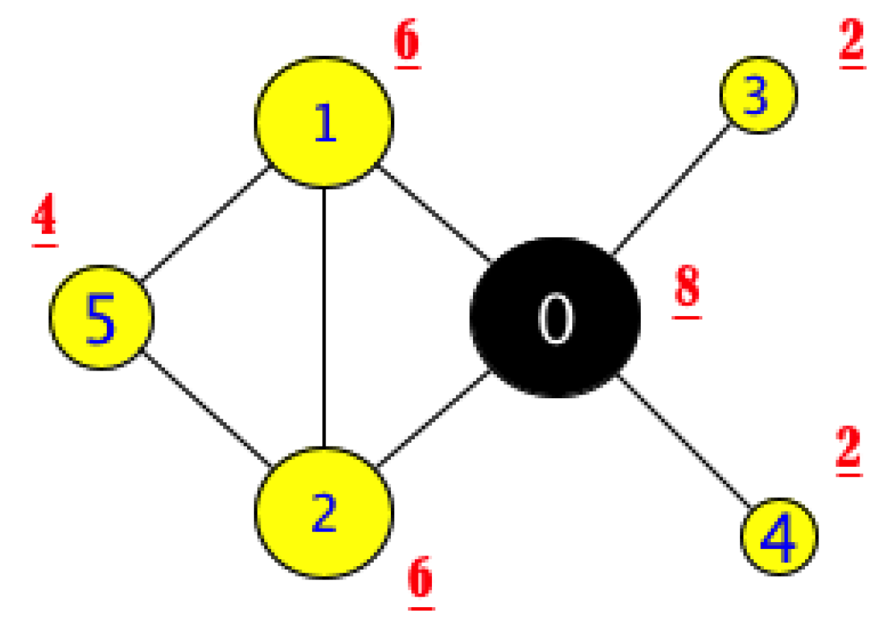
Consider, for instance, the node 0 in the graph of Figure 1a, which has been drawn again in Figure 2, and $\alpha =0.5$. For sake of simplicity, in the figure the bound $B(.)$ for each node is given in red underlined text. According to Theorem 2, an upper bound for node 0 is $B\left(0\right)=8$, then, $C^{*}\left(0\right)\le 8$. This bound is reached if and only if all of the neighbors of node 0 are in $C^{*}\left(0\right)$. The minimal required degree for an $\alpha$-quasi-clique of size 8 is 4 (according to Equation (4) in Theorem 2), whereas nodes 1, 2, 3, and 4 can be connected to, at most, 3, 3, 1, and 1 nodes, respectively (because of their degrees). We deduce that the upper bound cannot be achieved and $C^{*}\left(0\right)<8$. Indeed, by carefully examining Figure 2, one can easily deduce that $C^{*}\left(0\right)=\{0,1,2,5\}$, which is a community of size 4. Thus, the neighbors of 0 with the low degree (i.e., with low bound), nodes 3 and 4, are not members of the optimal community.

From this example, we conclude that, for a node having neighbors with a degree lower than its own degree, the bound given in Theorem 2 cannot be achieved.

In general, for any node $n_0$, $B\left(n_0\right)$ is reached if and only if all its neighbors are part of $C^{*}\left(n_0\right)$. In that case, $C^{*}\left(n_0\right)$ would be also upper bounded by ${\displaystyle \underset{n\in \Gamma \left(n_0\right)}{min}}B\left(n\right)$ (the lowest bound among all of the neighbors’ bounds). For our example, this is incompatible as the optimal solution is $C^{*}\left(0\right)=4$, whereas ${\displaystyle \underset{n\in \Gamma \left(0\right)}{min}}B\left(n\right)=2$ (bound of nodes 3 and 4).

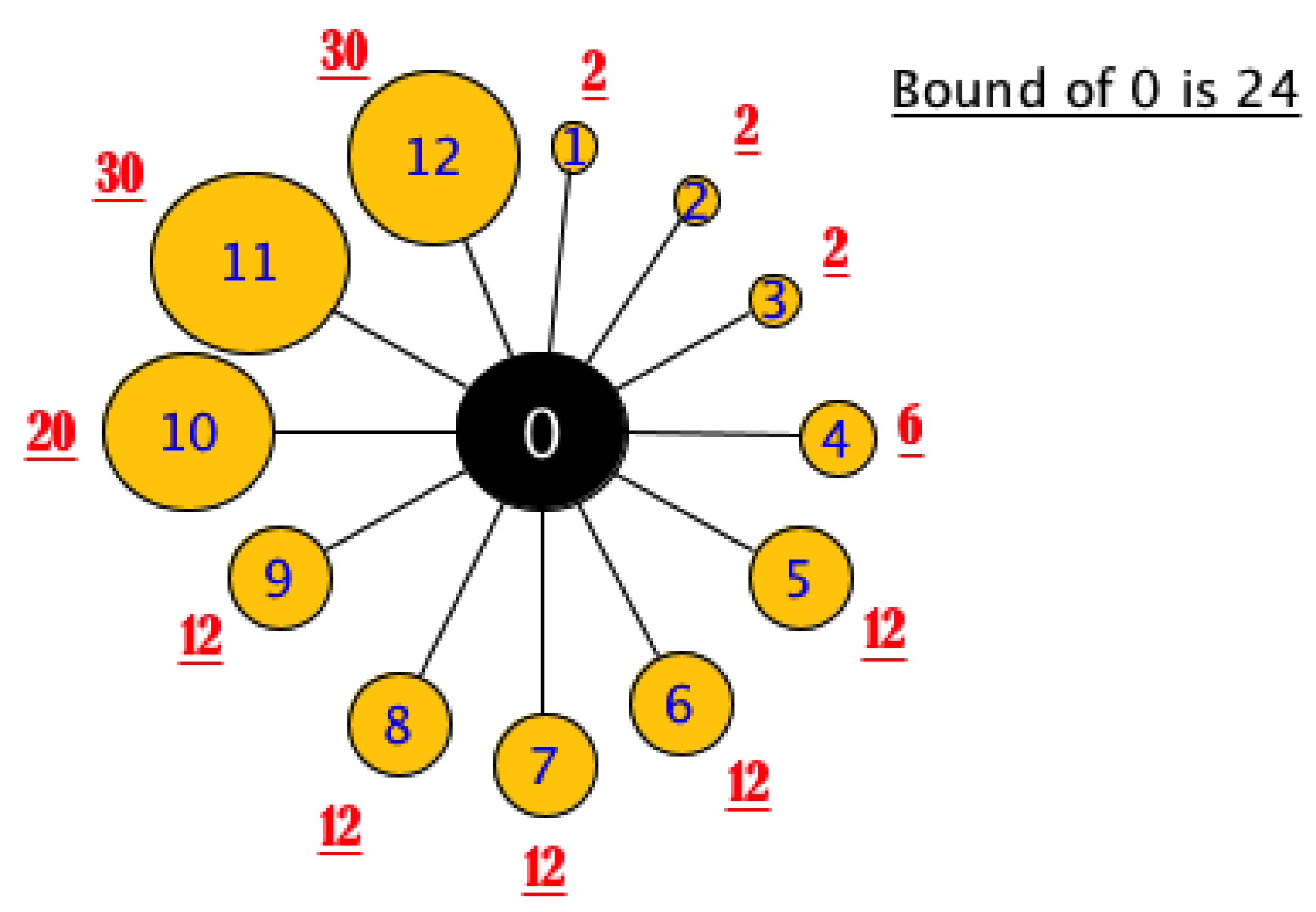
Let us formalize all of these ideas with a bigger graph. Consider a node with 12 neighbors, like the node 0 that is represented in Figure 3 and $\alpha =0.5$. In the figure, the size of each node has been drawn proportional to its degree (i.e., its bound). For each neighbor the upper bound (calculated basing on Theorem 2 for $\alpha =0.5$) is written in red underlined text. To simplify only the edges between node 0 and its neighborhood have been drawn. Without loss of generality, the node labels were attributed in ascending order according to the degree of each node. Notice that the bound $B\left(0\right)=24$ cannot be achieved, since 10 neighbors have an upper bound smaller than 24. Indeed, as we will see in the next subsection, the optimal upper bound for this example is 12.

3.3. The Algorithm

The algorithm to obtain an upper bound for the maximal α-quasi-clique community of a given node problem is divided in two main parts:

• Part I: “Improvements”: described in Algorithm 1, it includes the definition of the first and second neighborhood graph of $n_0$, ${\Gamma }_{12}\left(n_0\right)$; the initialization of the upper bounds for all nodes in ${\Gamma }_{12}\left(n_0\right)$ according to Theorem 2, along all the steps these values will be updated and saved in a table $\mathbf{B}$; finally, the search of improvements in the values of bounds is iteratively performed until no improvement is detected using the function bound() described in Part II. There is an improvement if the bound of at least one node in ${\Gamma }_{12}\left(n_0\right)$ has diminished.

Algorithm 1 Part I: Iterative improvements in the bound calculation.

Require: The graph $G(V,E)$, a node $n_0\in V$ and a parameter $\alpha$.

Ensure: An upper bound for the local $\alpha$-quasi-clique community size of node $n_0$.

1: Define the sub-graph ${\Gamma }_{12}\left(n_0\right)$.

2: for each node v in ${\Gamma }_{12}\left(n_0\right)$ do

3:   Set $\mathbf{B}\left[v\right]=B\left(v\right)$ (according to Equation (3) in Theorem 2).

4: end for

5: while there is at least one improvement do

6:  for each node v in ${\Gamma }_{12}\left(n_0\right)$ do

7:    if $\mathit{bound}(\Gamma (v),v,\mathbf{B},\alpha )<B\left[v\right]$  then

8:      $B\left[v\right]=\mathit{bound}({\Gamma }_{12},v,\mathbf{B},\alpha )$

9:      There is an improvement

10:    end if

11:  end for

12: end while

13: return  $\mathbf{B}\left[n_0\right]$

• Part II: thebound()function: described in Algorithm 2, this function calculates the bound for a given node per se taking into account the bounds of its neighbors. It takes four input parameters: the node $n_0$, its neighborhood graph ${\Gamma }_{12}\left(n_0\right)$, the table of bounds $\mathbf{B}$ and $\alpha$. First, a frequency distribution table of neighbors’ bounds is elaborated. These values are denoted $B_i^{neigh}$ and the associated frequency $f_i$ for i ranging from 1 to p, where p denotes the total number of different values of neighbor bounds (for instance, see

  Table 1. Frequency distribution of bound B for the neighbors of node 0 in Figure 3.

  Iteration i	Value of Bound ${\mathit{B}}_{\mathit{i}}^{\mathbf{neigh}}$	Frequency ${\mathit{f}}_{\mathit{i}}$	Remaining Degree ${\mathit{d}}_{\mathit{r}}$	Bound ${\mathit{B}}_{\mathit{i}}$	Neighbors ${\mathit{N}}_{\mathit{i}}$
  0	-	-	12	24	2
  1	2	3	9	18	3
  2	6	1	8	16	3
  3	12	5	3	6	9
  4	20	1	2	4	9
  5	30	2	0	0	12

  for the graph in Figure 3). Throughout the function, the bound of $n_0$ is denoted B and initially set to $B\left(n_0\right)$. At each iteration i, three values are updated: $d_r$, $B_i$, and $N_i$:

  -

  $d_r$ is the remaining degree and corresponds to the degree (number of connections) of $n_0$ resulting from disregarding the neighbors having the bound smaller or equal to $B_i^{neigh}$.

  -

  $B_i$ is a value of bound calculated using Theorem 2 and considering as input the remaining degree $d_r$ in Equation (3) instead of $d_0$. That is:

  $$\forall \mathrm{iteration}i{B}_i=\lceil \left(\frac{d_r}{\alpha }\right)\rceil \mathrm{and}{d}_r=\left(d\left(n_0\right)-\sum _{j=1}^i{f}_j\right).$$

  (5)

  -

  $N_i$ is the number of neighbors that can satisfy the bound $B_i$, that is, their bound is greater or equal to $B_i$.

At iteration 0 the initial values are $d_r=d\left(n_0\right)$, $B_0=B\left(n_0\right)$.

One can remark that there can be as many iterations as p.

The algorithm stops when a feasible solution is found. That is, when the remaining degree is maximal and such that there are at least enough neighbors that can satisfy the bound associated to such a value of remaining degree (rigorously, it is the value of $d^{min}=(\lfloor \alpha \left(\right|B_i|-1)\rfloor +1)$ that must be compared to $N_i$ because the purpose is to compare the minimal requirement of connections to the existing ones. However, this value turns out to be the remaining degree $d_r$), mathematically that means, $d_r\le N_i$.

Algorithm 2 The function bound().

Require: A node $n_0$, its neighborhood $\Gamma \left(n_0\right)$, the table of neighbors’ bounds $\mathbf{B}$ and a parameter $\alpha$.

Ensure: An upper bound B for the local $\alpha$-quasi-clique community size of node $n_0$.

1: Calculate the frequency distribution of neighbors’ bounds $\mathbf{B}\left(v\right)\forall v\in \Gamma \left(n_0\right)$, the resulting values

are denoted $B_i^{neigh}$ and the associated frequency $f_i$ ($\forall i\in \{1,\cdots ,p\}$).

2: // Initialize the iterations

3: Set $B=B\left(n_0\right)$, $i=0$, $d_r=d\left(n_0\right)$, $B_0=B\left(n_0\right)$ and calculate $N_0$ (number of neighbors whose bound

is at least equal to $B_0$).

4: while$(d_r>N_i)$do

5:  i=i+1

6:  Update $d_r=(d_r-f_i)$ and $B_i=\lceil \left(\frac{d_r}{\alpha }\right)\rceil$, calculate $N_i$

7:  if $B_i\le B_i^{neigh}$  then

8:   $B=B_i^{neigh}$

9:   Break

10:  else

11:   $B=B_i$

12:  end if

13: end while

14: returnB

For our example in Figure 3, the frequency distribution table of the upper bounds for all the neighbors is given in Table 1. There are, in total, $p=5$ different values (2, 6, 12, 20, and 30) with their associated frequencies 3, 1, 5, 1, and 2, respectively. At the beginning, we have $B=B\left(0\right)=24$, $d_r=d\left(0\right)=12$ and $B_0=24$. Only 2 neighbors satisfy the bound $B_0$, that is, nodes labeled 11 and 12, then $N_0=2$. Thus, the bound $B_0$ can not be achieved, since $d_r>N_0$ and the iterations in the while loop start:

• $i=1$, $d_r=9$ (after disregarding nodes 1, 2, and 3), $B_1=18$, $N_1=3$ (nodes 10, 11 and 12). Since $B_1=18>B_1^{neigh}=2$, then $B=18$; $d_r>N_1$, then we iterate once more.
• $i=2$, $d_r=8$ (after ignoring nodes 1, 2, 3, and 4), $B_2=16$, and $N_2=3$ (nodes 10, 11 and 12). Because $B_2=16>B_2^{neigh}=6$, then $B=16$; $d_r>N_2$, we continue....
• $i=3$, $d_r=3$ (after ignoring nodes 1, 2, 3, 4, 5, 6, 7, 8, and 9), $B_3=6$, and $N_3=9$ (nodes 4, 5, 6, 7, 8, 9, 10, 11, and 12). Because $B_3=6<B_3^{neigh}=12$, then $B=B_3^{neigh}=12$ and the algorithm exits the while loop following the break statement.

At this iteration, the algorithm stops and returns $B=12$. Therefore, a feasible an maximal solution has been detected, indeed, eight neighbors have a bound greater or equal to 12 and only six are needed according to Equation (4) in Theorem 2.

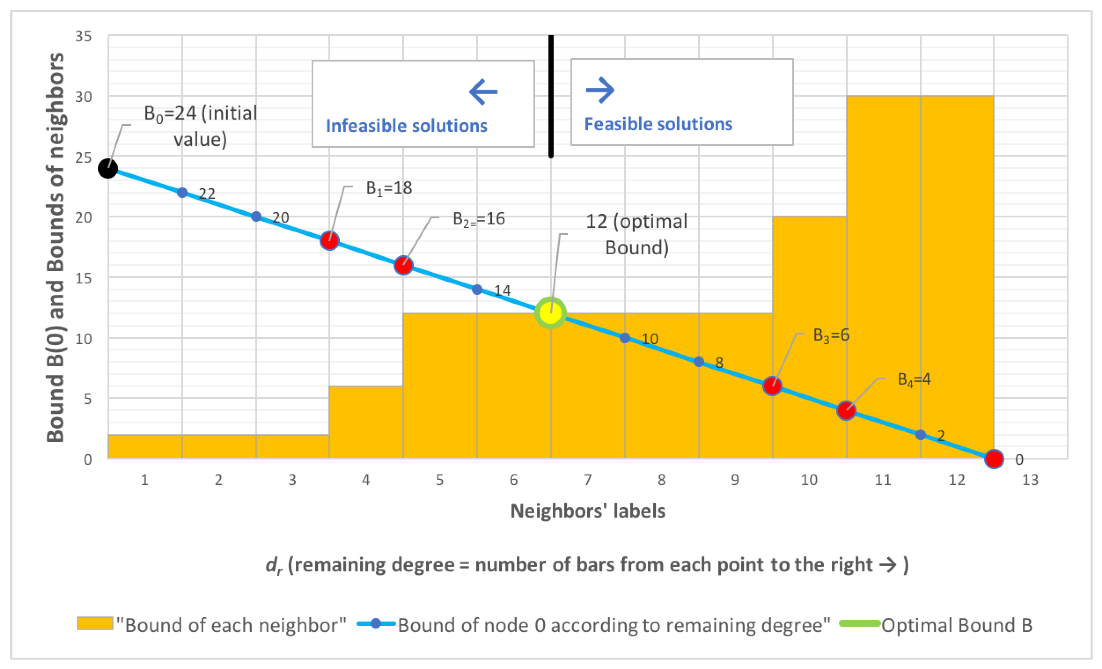
For the sake of interpretation, the graphical execution of the algorithm is given in Figure 4. In the figure, the points on the blue line present the bound $B_i$ calculated for each value of remaining degree (according to Equation (5)). We consider, on the left, no neighbor is ignored, so the remaining degree is maximal and equal to $d_r=d\left(0\right)=12$, whereas on the right all neighbors are ignored and $d_r=0$. The bars in orange present the bound for each neighbor according to its labels given in the horizontal axis. This bar chart looks like a staircase increasing function where each step represents each value of neighbor bound $B_i^{neigh}$. The optimal value of bound is found when both, the line and the bar chart, intersect for the first time. The progress of iterations are given from left to right, thus at the beginning there are not enough neighbors to satisfy the bound B. As we move from left to right the value of bound B decreases whereas the available neighbors have higher bounds, up to a feasible solution is achieved. For this example, the optimal value, $B=12$, is found in iteration 3. Indeed, just before, in iteration 2 we have $B=16$, $d_r=8$ and $N_3=3$ (i.e., only 3 neighbors have bound great or equal to 16). The values $N_i$ can be determined from the graphic by imagining an horizontal line that intercepts the blue line at a given iteration and counting the number of bars that are intersected. For instance, at iteration 2 the horizontal line cut the vertical axis at 16 and intersects the bars representing neighbors 10, 11 and 12 (the neighbors that satisfy bound $B_2=16$), then $N_2=3$. Bounds $B_3=6$ and $B_4=4$ are feasible solutions but they are not maximal.

The proposed algorithm calculates the optimal upper bound by initializing it with a high value and then iteratively reducing it until a feasible solution is found. It is important to highlight that the optimal bound can also be obtained by starting with low values, for instance 0, and then, iteratively increasing it just before an unfeasible solution is obtained. For our example in Figure 4, this comes back to consider the values $B_i^{neigh}<12$, which is 0, 4, and 6.

Furthermore, the graphical solution that is presented in Figure 4 can be very useful. Indeed, all of the points on the line show the values of bound B for a given value of remaining degree $d_r$, which can be obtained by counting the number of bars from a given point to the right, this value corresponds to the number of required connections to achieve B. Besides, as discussed above, given a point on the line, the number of connections that satisfy the bound $N_i$ can also be read from the graphic. For instance, if for any i we have $B_i=14$, then $d_r=7$ and $N_i=3$. These interpretations from the graphic lead us to a simple way to obtain the optimal value of bound. Certainly, for any value of bound B on the line, it is necessary to look for the point where the line intersects the bars, from that point to the right all of the solutions are feasible. In contrast, from that point to the left all the solutions are unfeasible. Then, the optimal bound takes place always in the intersection. For any node with degree $d>0$, the line of bounds is decreasing and always intersects the horizontal axis in the point ($B=0$, $d_r=0$). This guarantees that the line always intersects the bars, the only exception is the case when all of the neighbors have a bound higher than that of the starting node. However, in that case, the optimal bound is equal to the starting value, that is $B=B\left(n_0\right)$ with $d_r=d\left(n_0\right)$, as given in Equation (3) from Theorem 2.

3.4. Complexity

The calculations of complexity are given for the worst case scenario.

We start by calculating the complexity of the bound() function, which is, the calculation of the upper bound per se. By carefully examining the steps in Algorithm 2, we can see that there are two main time consuming operations:

• The calculation of the frequency table implies to sort the values of neighbors’ bounds and count the frequencies. This operation requires the necessary time to sort p values, since p is, at most, $|\Gamma \left(n_0\right)|=d_0$. Depending on the sorting algorithm in the worst case, this operation can perform in $\mathcal{O}\left(d_0^2\right)$.
• The operations in the while loop (lines 4 to 13) to find the optimal value of bound can be executed using a binary search algorithm. Certainly, the purpose is to find a value in the frequency table of sorted neighbors’ bounds. Indeed, each row in the frequency table (see Table 1) corresponds to a step in the staircase bar chart diagram in Figure 4. The purpose is to determine the step (iteration) i, where the line intersects the bar chart. The values $B_i$, $d_r$ and $N_i$ can be directly calculated from the frequency table. Given a step i with its corresponding value of $d_r$, one of the following situations can take place:

  —

  $N_i<d_r$ implies block i is in the area of unfeasible solutions, then, the search must continue in the blocks corresponding to greater values of i (to the right following the blue line in the graphic).

  —

  $N_i=d_r$ implies the optimal bound is $B=B_i$.

  —

  $N_i>d_r$ implies block i is in the area of feasible solutions. However, it is necessary to verify whether we are in the block of the maximal solution. If and only if $N_{i-1}<d_r(i-1)$, the optimal bound is $B=B_i^{neigh}$; otherwise, the search must continue in the blocks corresponding to smaller values of i (to the left following the blue line in the graphic).

For the example graph in Figure 4, we need only one iteration using Binary search. We have $p=5$, then the initial value $i=3$ (the value in the middle of Table 1). We set $N_3=9$, $d_r=3$, then $N_i>d_r$, which means that block 3 is in the area of feasible solutions but it is possible to improve. Next, we notice $N_2<d_r\left(2\right)$ ($3<8$) and conclude that the optimal bound is $B=B_3^{neigh}=12$.

This operation runs in $\mathcal{O}(log(p\left)\right)$, since p ranges from 1 to $d_0$, then we have complexity $\mathcal{O}(log\left(d_0\right))$ in the worst case.

Finally, the complexity of the bound() function for a node $n_0$ with degree $d_0$ is: $\mathcal{O}\left(d_0^2\right)+\mathcal{O}(log\left(d_0\right))=\mathcal{O}\left(d_0^2\right)$. That is, the most consuming time operation is the elaboration of the frequency table.

Now, let us focus on the complexity of the algorithm of improvements, described in Algorithm 1. The loop of improvements is the most time consuming task, previously, there are two operations:

• The definition of the first and second neighborhood graph ${\Gamma }_{12}\left(n_0\right)$ which runs in $\mathcal{O}(d_0+{\sum }_{v\in \Gamma \left(n_0\right)}{d}_v)$. Indeed, the definition of the first neighborhood needs $|\Gamma \left(n_0\right)|=d_0$ operations. Subsequently, to extract the second neighborhood, for each neighbor v, $d_v$ operations are needed.
• The calculation of the initial upper bound for all the nodes in ${\Gamma }_{12}\left(n_0\right)$ using Equation (3) from Theorem 2 requires $\mathcal{O}\left(\right|{\Gamma }_{12}\left(n_0\right)\left|\right)$ operations.

Finally, let us consider the most onerous task of the whole algorithm, that is the while loop of improvements. At each pass the function bound() in Algorithm 2 is executed for all the nodes in ${\Gamma }_{12}\left(n_0\right)$. As we have seen above, for each node v this runs in $\mathcal{O}\left(d_v^2\right)$. Afterwards, one iteration runs in time ${\sum }_{v\in {\Gamma }_{12}\left(n_0\right)}\left(d_v^2\right)$. Now, the issue is to determine how many iterations we need. We consider there is an improvement if at least for one node in ${\Gamma }_{12}\left(n_0\right)$ its bound has been reduced by at least one unit. In the worst case scenario, at each iteration there is only one improvement for one node by only one unit, which means that, for a node v we can have at most $\left(\lceil \left(\frac{d\left(v\right)}{\alpha }\right)\rceil \right)$ iterations. Finally, the complexity of our algorithm becomes ${\displaystyle \mathcal{O}\left(\sum _{v\in {\Gamma }_{12}\left(n_0\right)}\lceil \left(\frac{d\left(v\right)}{\alpha }\right)\rceil \sum _{v\in {\Gamma }_{12}\left(n_0\right)}\left(d_v^2\right)\right)}$.

We remark the iterative improvements might be very time consuming. However, as we will see in Section 4, for real networks important improvements take place during the very early iterations.

4. Experimental Results

This section is divided in three subsections. First, we evaluate the bound with a small real network for which it is possible to calculate the optimal solution of Problem 1 for all the nodes. Next, we compare the proposed bound to the baseline version studied in [12]. Finally, we consider the impact of the iterative improvements part of the algorithm on the final value of the bound since it is the most time consuming part.

All of the evaluations are performed using the following four real networks commonly used in social network analysis. All these datasets are publicly available online (please, see [29] for the details):

• “The Zachary Karate Club network” (karate) [30]: a network of members of a karate club at a US university in the 1970s, 34 nodes and 78 edges.
• “The American College football network” (football) [31]: a network of American football games between colleges during regular season Fall 2000, 115 nodes and 613 edges.
• “Books about US politics” (polbooks) [32]: a network of books about US politics published around the time of the 2004 presidential election and sold by the online bookseller Amazon.com. Edges between books represent frequent co-purchasing of books by the same buyers, 105 nodes and 441 edges.
• “Political blogs” (polblogs) [33]: a network of hyperlinks between weblogs on US politics, 1224 nodes and 16715 edges.

4.1. Evaluation of the Bound in a Small Real Network

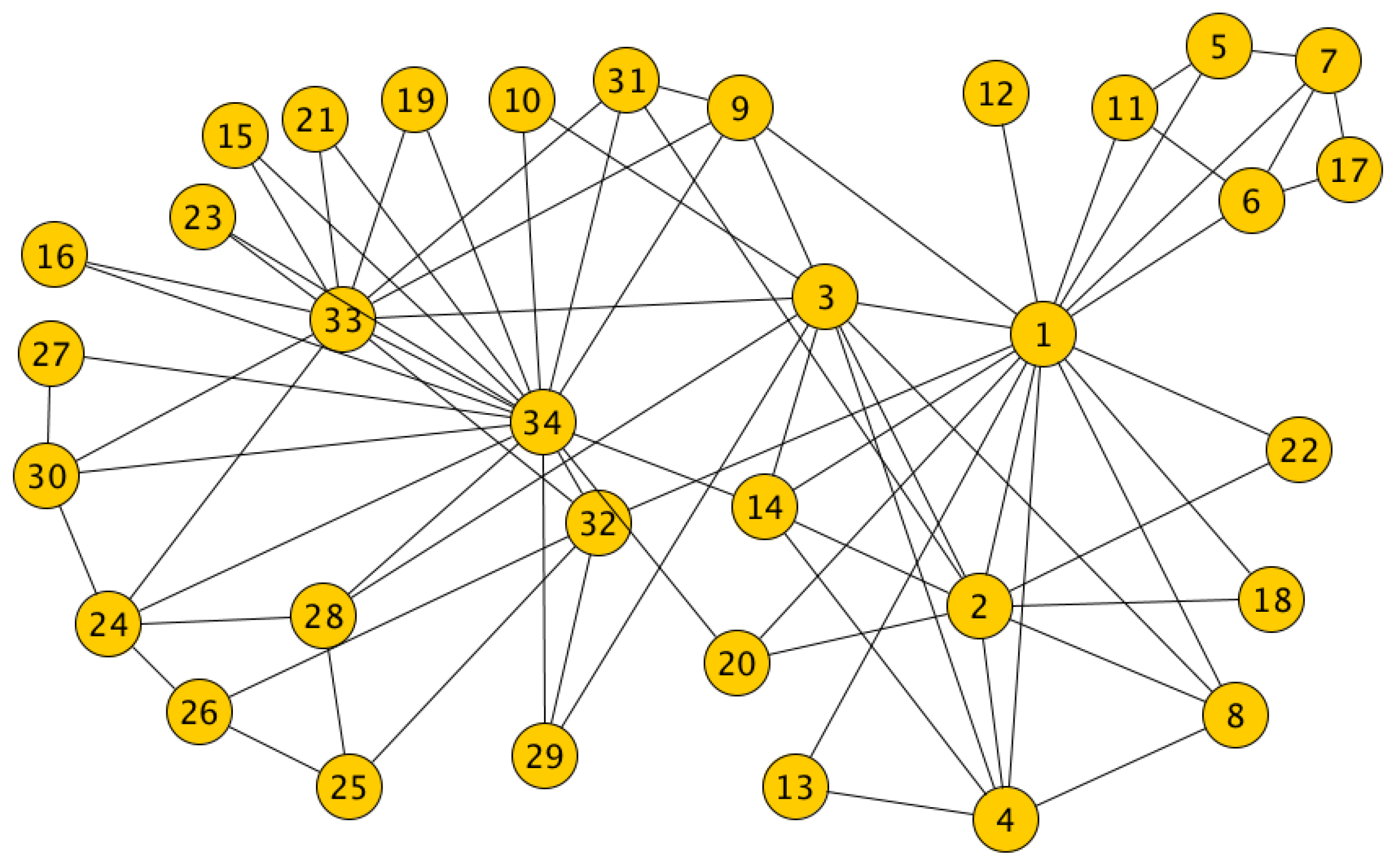
We study deeply the karate network since the optimal solution for the maximal α-quasi-clique community of a given node problem can be exactly determined for every node in such a small network. To simplify, we consider $\alpha =0.5$. Indeed, in this situation, the calculation of the upper bound given in Equation (2) turns out to multiply by two the degree of the node. The Figure 5 shows the karate network.

Table 2. Results for the karate network.

Difference between the Bound and the Optimal Value	Number of Nodes	Percentage of Nodes	Concerning Nodes
0	28	82 %	-
1	4	12 %	4 and 8
2	2	6%	5, 6, 7 and 11
TOTAL	34	100%	-

presents the frequency table of the difference between the upper bound and the optimal community size value. If the difference is 0, then the bound returns exactly the optimal value.

We can see from Table 2 that the algorithm is exact for 82% of the nodes. That is, the upper bound is completely accurate. Concerning the remaining 18%, the difference between the bound and the optimal value is either 1 or 2. Now, we will deeply analyze these cases.

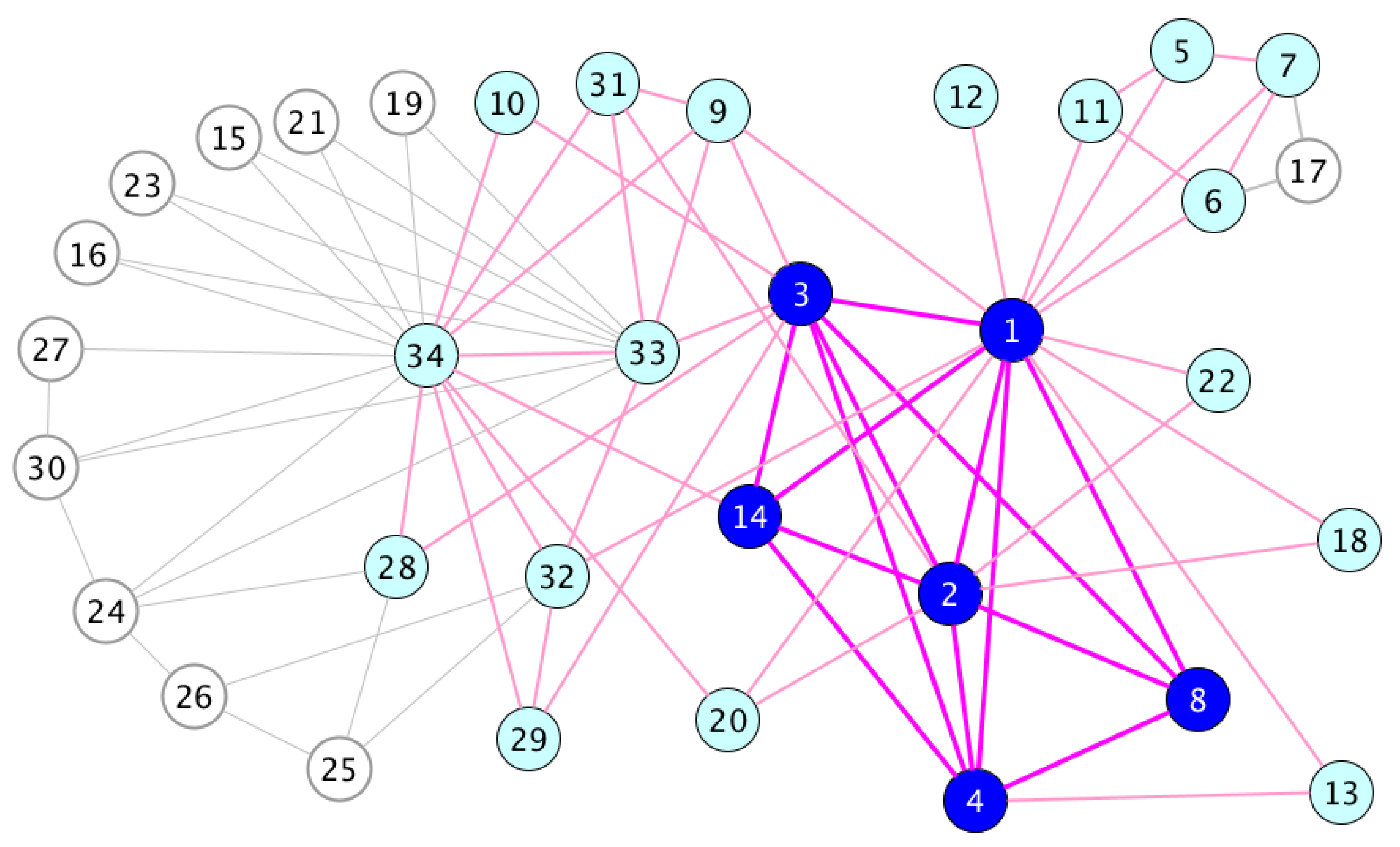
Figure 6 shows the optimal local community for node 4 (the same for node 8), which is, the maximal $0.5$-quasi-clique containing that node is of size 6. However, the upper bound returned by our method is 8. Accordingly, there is a gap of two units. From the figure, we can remark that all the neighbors of node 4 (the same for node 8) have a degree of at least 4, which is exactly the required minimal degree for a community of size 8 (see Equation (4)). Furthermore, the optimal community is nearly a complete clique, which is, by carefully examining the members of the optimal community they all have an internal degree greater or equal to 4, whereas $d^{min}=3$ for a community of size 6. The proposed bound tends to exceed the optimal value in such a situation, since there is no indication to conclude that the optimal community is smaller than 8. However, by inspecting the figure, no node among the nodes in light blue would satisfy the rule of an $\alpha$-alpha-quasi-clique if it became member of the local community.

In addition, Figure 6 allows illustrating another advantage of our algorithm. All of the nodes being part of ${\Gamma }_{12}\left(4\right)$ are colored either in dark or light blue. Only considering this subgraph (instead of the whole graph) to solve problem 1 considerably reduces the search space, since central nodes having a high degree in the whole graph have fewer connections in the resulting subgraph ${\Gamma }_{12}$, such as node 34.

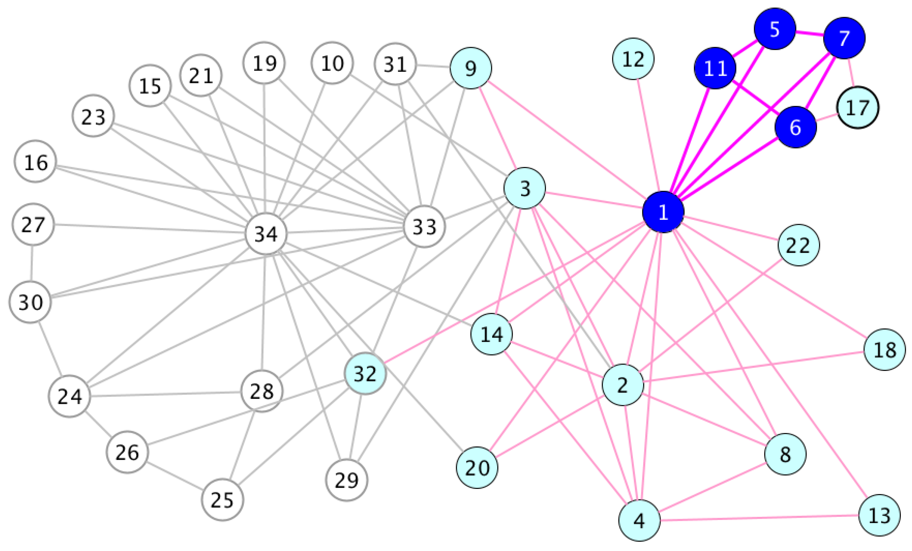
Now, consider nodes 5, 6, 7, and 11. Figure 7 presents the optimal solution for each of those nodes as well as the first and second neighborhood graph. The optimal community that solves Problem 1 containing each of these nodes is of size 5, whereas the upper bound that is returned by the algorithm is 6. First of all, it is important to highlight that, when $\alpha =0.5$, the proposed algorithm can only return even numbers as the calculations are based on Equation (2). Subsequently, if the optimal solution corresponds to an odd number and $\alpha =0.5$, the bound cannot be achieved. Fortunately, this situation only arises for $\alpha =0.5$. Furthermore, idem to nodes 4 and 8, there is no indication to deduce that the optimal community is smaller than 6. However, we can see that the internal degree of four nodes (5, 6, 7, and 11) is equal to the minimal internal degree for a community of size 5 that is 3 (see Equation (4)). Moreover, nodes 5 and 11 have degree 3. This can be an indicator that the value is close to the optimal solution for any heuristic that returns a community of odd-sized.

4.2. Comparison of the Proposed Bound to the Baseline Version

Now, we will study the impact of considering the first and second neighborhood subgraph, instead of the whole graph, in the bound calculation in order to compare the bound to the baseline version in [12].

For the four real networks, Figure 8 and Figure 9 present the boxplots of the size of the 1st- and 2nd-neighborhood subgraph, ${\Gamma }_{1,2}(.)$ in terms of number of nodes and number of edges respectively for every node in each network. In each plot, the value of the total number of nodes N and the total number of edges M in the whole network is given and represented by a horizontal line.

Figure 8 and Figure 9 show that the search space is reduced for all the nodes in the four networks, in terms of both, the number of nodes and the number of edges. One can remark that for the football and polbooks networks the ${\Gamma }_{12}(.)$ subgraph is even about half the size of the entire network for all the nodes. For some nodes the ${\Gamma }_{12}(.)$ graph is really small, for instance, in the polbooks and polblogs networks; on the other hand, for some exceptional nodes in karate and polblogs the search space can even get close in size to the whole network, for instance, this happens for some nodes that occupy a central position, which is, they have a high degree.

Now, we will compare the value of the proposed bound to the baseline method bound. For the four real networks and different values of $\alpha$, Figure 10 compares the bound obtained by executing the algorithm taking as input the whole graph G to that obtained taking as input ${\Gamma }_{12}(.)$ for each of the nodes in those networks. More specifically, the difference, called Gain between these two values, is calculated. This implies to execute the function bound() (described in Algorithm 2) with input parameters $n_0$, $\Gamma \left(n_0\right)$, $\alpha$ and the table of bounds $\mathbf{B}$ calculated based on the whole G in the first case and based on the ${\Gamma }_{12}$ subgraph in the second case. To allow the comparison only one iteration of the improvements part described in Algorithm 1 is performed. That is, only one pass in the while loop. Each bar in the figure represents the percentage of nodes for which both bounds are equal (in green, Gain = 0) and the complement, which is, the percentage of nodes for which the proposed bound is tighter that the one calculated based on the whole graph (in red, Gain $>0$).

We can see from the Figure 10 that the proposed bound is, in all cases, more accurate for all of the datasets. The results do not seem to vary a lot for the different values of $\alpha$. This can be explained by the fact that the frequencies in the frequency table elaborated in the bound() function do not vary from one value of $\alpha$ to another one. We can also see that for the football dataset there is a refinement of the bound in about 90% of cases. For polbooks and polblogs in about 30% of cases the proposed bound is tighter (more specifically 33% for polbooks).

4.3. Impact of the Iterative Improvements

At present, let us focus on the impact of the iterative improvements performed during the execution of the algorithm (while loop in Algorithm 1).

Table 3. Table of improvements per iteration for three real networks, values are given in percentage (%).

karate, $\mathit{\alpha }=0.5$					football, $\mathit{\alpha }=0.5$									polblloks, $\mathit{\alpha }=0.5$
	Improvement					Improvement									Improvement
it	0	1	2	TI	it	0	1	2	3	4	5	6	TI	it	0	1	2	3	4	5	6	TI
1	100	-	-	0	1	100	-	-	-	-	-	-	0	1	100	-	-	-	-	-	-	0
2	91	-	9	9	2	49	-	36	-	12	-	3	51	2	66	-	25	-	8	-	2	34
3	44	-	-	0	3	95	-	3	-	-	-	-	3	3	80	-	15	-	-	-	-	15
					4	33	-	4	-	-	-	-	4	4	75	-	1	-	-	-	-	1
					5	14	-	-	-	-	-	-	0	5	35	-	-	-	-	-	-	0
					6	5	-	-	-	-	-	-	0
					7	2	-	-	-	-	-	-	0
					8	-	-	1	-	-	-	-	1
					9	1	-	-	-	-	-	-	0
karate,$\mathbf{\alpha }=\mathbf{0.8}$					football,$\mathbf{\alpha }=\mathbf{0.8}$									polblloks,$\mathbf{\alpha }=\mathbf{0.8}$
	Improvement					Improvement									Improvement
it	0	1	2	TI	it	0	1	2	3	4	5	6	TI	it	0	1	2	3	4	5	6	TI
1	100	-	-	0	1	100	-	-	-	-	-	-	0	1	100	-	-	-	-	-	-	0
2	91	3	6	9	2	49	23	15	10	3	-	-	51	2	66	18	9	6	2	-	-	34
3	44	-	-	0	3	95	3	-	-	-	-	-	3	3	80	14	1	-	-	-	-	15
					4	33	4	-	-	-	-	-	4	4	75	1	-	-	-	-	-	1
					5	14	-	-	-	-	-	-	0	5	35	-	-	-	-	-	-	0
					6	5	-	-	-	-	-	-	0
					7	2	-	-	-	-	-	-	0
					8	-	1	-	-	-	-	-	1
					9	1	-	-	-	-	-	-	0

and

Table 4. Table of number of improvements per iteration for the polblogs network, $\alpha =0.5$.

	Amount of Improvement
it	0	2	4	6	8	10	12	14	16	18	20	22	24	26	28	30	32	34	36	38	44	TI (%)
1	1224	-	-	-	-	-	-	-	-	-	-	-	-	-	-	-	-	-	-	-	-	0
2	819	113	62	48	45	21	24	11	24	17	7	9	5	5	3	2	1	2	1	1	2	33
3	931	103	73	55	26	4	-	1	-	-	-	-	-	-	-	-	-	-	-	-	-	21
4	1003	99	73	6	-	-	-	-	-	-	-	-	-	-	-	-	-	-	-	-	-	15
5	1019	110	7	-	-	-	-	-	-	-	-	-	-	-	-	-	-	-	-	-	-	10
6	993	88	-	-	-	-	-	-	-	-	-	-	-	-	-	-	-	-	-	-	-	7
7	932	60	-	-	-	-	-	-	-	-	-	-	-	-	-	-	-	-	-	-	-	5
8	791	61	-	-	-	-	-	-	-	-	-	-	-	-	-	-	-	-	-	-	-	5
9	706	7	-	-	-	-	-	-	-	-	-	-	-	-	-	-	-	-	-	-	-	1
10	513	4	-	-	-	-	-	-	-	-	-	-	-	-	-	-	-	-	-	-	-	0
11	355	-	-	-	-	-	-	-	-	-	-	-	-	-	-	-	-	-	-	-	-	0
12	173	-	-	-	-	-	-	-	-	-	-	-	-	-	-	-	-	-	-	-	-	0
13	60	-	-	-	-	-	-	-	-	-	-	-	-	-	-	-	-	-	-	-	-	0
14	28	-	-	-	-	-	-	-	-	-	-	-	-	-	-	-	-	-	-	-	-	0
15	17	1	-	-	-	-	-	-	-	-	-	-	-	-	-	-	-	-	-	-	-	0
16	6	-	-	-	-	-	-	-	-	-	-	-	-	-	-	-	-	-	-	-	-	0
17	5	-	-	-	-	-	-	-	-	-	-	-	-	-	-	-	-	-	-	-	-	0
18	3	-	-	-	-	-	-	-	-	-	-	-	-	-	-	-	-	-	-	-	-	0
19	1	-	-	-	-	-	-	-	-	-	-	-	-	-	-	-	-	-	-	-	-	0

show the amount of improvement in the value of bound in units (denoted Improvement) per number of iteration (denoted it). Table 3 is composed of six subtables, each one corresponds to a given network and a value of $\alpha$. Since there is no so much variability, we chose only two values of $\alpha$, 0.5 and 0.8. For a given subtable, each entry represents the percentage of nodes in the whole network for which the bound has decreased in the units given by the improvement value at a given iteration. For instance, for 36% of nodes in the football network the bound has decreased by two units at iteration 2 (relative to iteration 1). The last column of each subtable presents the total percentage of nodes for which there was an improvement of any amount at a given number of iteration, denoted TI. The numbers are given in bold whenever some improvement took place for at least one node. For instance, in total for 51% of nodes in football, the bound experimented some improvement (then, it got closer to the optimal solution) at the second iteration.

Now let us comment the results in Table 3. Iteration 1 being the starting point, no improvement takes place. The number of iterations differs from one network to another one. In the football network, for one node there is an improvement of one unit, even at iteration 8. Analogous, for one node in polbooks the number of iteration goes up to 5. For the three networks, the amount of improvement is much more accentuated at the second iteration. For instance, for some nodes the bound decreases by even six units. This leads to new ideas in practice, such as early stopping at the first iterations; furthermore, the iterative improvements part is the most time consuming task in the whole method as discussed in Section 3.4. We consider it relevant to explain why at some iterations no improvements take place, for instance, this situation arises in about 14% of cases of the nodes in the football network at iteration 5. Just remind that, in the Algorithm 1, there is an improvement if at least for one node in ${\Gamma }_{12}(.)$ the bound has decreased, this node can be different from $n_0$. In Table 3 we count only the improvements for the target node $n_0$. One can also remark that there are no improvements at the final iteration which is quite normal since, whenever there is some an improvement, a supplementary iteration is performed.

Finally, we study the results for the polblogs network. The Table 4 shows the amount of improvements per number of iteration (it). Given the size of the network, the values are not given in percentage, except for the last column, TI.

We remark important improvements at second iteration, where for about 33% of nodes the bound becomes tighter. The amount of improvement goes up to 44 units. For one node there is an improvement of two units at the 15th iteration. For four nodes, there are still improvements at iteration 10. These results show that it is worth performing at least a second iteration pass or even third or forth, because for 21% and 15% of nodes, respectively, there are important improvements.

5. Conclusions and Perspectives

The present research provides a method to evaluate heuristics searching to approach the maximal α-quasi-clique community of a given node problem. This problem aims to detect subgraph of maximal size, containing a node of interest in the network. This subgraph or community must verify the constraints of an $\alpha$-quasi-clique, more specifically, each node must be connected to more than a proposition $\alpha$ of nodes in the community. This problem being NP-hard, existing methods to solve it are heuristics. We propose an upper bound for the optimal solution that allows measuring how close a proposed solution is to the optimal one. A theorem states that for high values of $\alpha$, (greater than $0.5$), the optimal solution has a diameter of at most 2. In this sense, given the starting node, we extract the subgraph containing the first and second neighborhood of the node, this returns a subgraph, where all nodes are at a distance of at most 2 of the starting node. Experimentally, we showed that this reduces considerably the value of the bound, so that, this latter gets tighter and gets closer to the optimal value. Our algorithm consists in two parts, one part serving to calculate the upper bound per se and another one performing iterative improvements. The experiments showed that a great amount of improvement takes place at the first iterations for the majority of the nodes, which suggested to early stop the algorithm if needed at first stages and allows for saving time in the execution. We also presented a graphical solution or visualization of how to calculate the upper bound.

The calculation of a bound for an $NP$-complete problem opens the door for interesting applications, for instance, heuristics that perform iterative calculations in order to approach the optimal solution must stop once the bound is reached. In such a situation, one can be sure that the algorithm reached the optimal solution.

One clue to improve the presented method is to try to reduce the diameter of the first and second neighborhood graph, which has a diameter of at most 4, whereas the optimal solution has, at most, a diameter of 2.

Another perspective for this work is to extend the Problem 1 to directed graphs. Indeed, this problem is designed only for undirected graphs where the links between nodes are symmetric. One idea would be to consider the definition of a clique for a directed graph where every two distinct nodes are connected to each other in both directions. In that case, the rule of an $\alpha$-quasi-clique should also be modified to consider both directions.

References

1. Fortunato, S. Community detection in graphs. Phys. Rep. 2010, 486, 75–174. [Google Scholar] [CrossRef] [Green Version]
2. Bomze, I.M.; Budinich, M.; Pardalos, P.M.; Pelillo, M. The Maximum Clique Problem. In Handbook of Combinatorial Optimization; Kluwer Academic Publishers: New York, NY, USA, 1999; pp. 1–74. [Google Scholar]
3. Lee, V.E.; Ruan, N.; Jin, R.; Aggarwal, C.C. A Survey of Algorithms for Dense Subgraph Discovery. In Managing and Mining Graph Data; Aggarwal, C.C., Wang, H., Eds.; Springer: Berlin/Heidelberg, Germany, 2010; Volume 40, pp. 303–336. [Google Scholar]
4. Pattillo, J.; Youssef, N.; Butenko, S. On clique relaxation models in network analysis. Eur. J. Oper. Res. 2013, 226, 9–18. [Google Scholar] [CrossRef]
5. Wu, Q.; Hao, J.K. A review on algorithms for maximum clique problems. Eur. J. Oper. Res. 2015, 242, 693–709. [Google Scholar] [CrossRef]
6. Newman, M.; Girvan, M. Finding and evaluating community structure in networks. Phys. Rev. E 2004, 69, 026113. [Google Scholar] [CrossRef] [PubMed] [Green Version]
7. Fortunato, S.; Barthelemy, M. Resolution limit in community detection. Proc. Natl. Acad. Sci. USA 2006, 104, 36–41. [Google Scholar] [CrossRef] [PubMed] [Green Version]
8. Karp, R.M. Reducibility Among Combinatorial Problems. In Complexity of Computer Computations; The IBM Research Symposia Series; Miller, R.E., Thatcher, J.W., Eds.; Plenum Press: New York, NY, USA, 1972; pp. 85–103. [Google Scholar]
9. Asahiro, Y.; Hassin, R.; Iwama, K. Complexity of Finding Dense Subgraphs. Discret. Appl. Math. 2002, 121, 15–26. [Google Scholar] [CrossRef] [Green Version]
10. Conde-Céspedes, P.; Ngonmang, B.; Viennet, E. Approximation of the Maximal α-Consensus Local Community detection problem in Complex Networks. In Proceedings of the IEEE SITIS 2015, Complex Networks and their Applications, Bangkok, Thailand, 23–27 November 2015. [Google Scholar]
11. Conde-Céspedes, P.; Ngonmang, B.; Viennet, E. An efficient method for mining the Maximal alpha-quasi- clique-community of a given node in Complex Networks. Soc. Netw. Anal. Min. 2018, 8. [Google Scholar] [CrossRef]
12. Conde-Céspedes, P. Local Community Detection of High Density: An Upper Bound for the Optimal Solution. Sens. Transducers 2019, 234, 37–43. [Google Scholar]
13. Abello, J.; Resende, M.G.C.; Sudarsky, S. Massive Quasi-Clique Detection. In Proceedings of the 5th Latin American Symposium on Theoretical Informatics (LATIN ’02); Springer: London, UK, 2002; pp. 598–612. [Google Scholar]
14. Chen, J.; Saad, Y. Dense Subgraph Extraction with Application to Community Detection. IEEE Trans. Knowl. Data Eng. 2012, 24, 1216–1230. [Google Scholar] [CrossRef]
15. Pattillo, J.; Veremyev, A.; Butenko, S.; Boginski, V. On the maximum quasi-clique problem. Discret. Appl. Math. 2013, 161, 244–257. [Google Scholar] [CrossRef] [Green Version]
16. Tsourakakis, C.; Bonchi, F.; Gionis, A.; Gullo, F.; Tsiarli, M. Denser Than the Densest Subgraph: Extracting Optimal Quasi-cliques with Quality Guarantees. In Proceedings of the 19th ACM SIGKDD International Conference on Knowledge Discovery and Data Mining (KDD ’13); ACM: New York, NY, USA, 2013; pp. 104–112. [Google Scholar]
17. Brunato, M.; Hoos, H.H.; Battiti, R. On Effectively Finding Maximal Quasi-cliques in Graphs. In LION; Maniezzo, V., Battiti, R., Watson, J.P., Eds.; Springer: Berlin/Heidelberg, Germany, 2007; Volume 5313, pp. 41–55. [Google Scholar]
18. Liu, G.; Wong, L. Effective Pruning Techniques for Mining Quasi-Cliques. In Machine Learning and Knowledge Discovery in Databases; Daelemans, W., Goethals, B., Morik, K., Eds.; Springer: Berlin/Heidelberg, Germany, 2008; Volume 5212, pp. 33–49. [Google Scholar]
19. Chou, Y.H.; Wang, E.T.; Chen, A.L.P. Finding Maximal Quasi-cliques Containing a Target Vertex in a Graph. In DATA2015, Proceedings of 4th International Conference on Data Management Technologies and Applications—Volume 1: DATA; INSTICC, SciTePress: Setubal, Portugal, 2015; pp. 5–15. [Google Scholar] [CrossRef]
20. Lee, P.; Lakshmanan, L.V.S. Query-Driven Maximum Quasi-Clique Search. In Proceedings of the 2016 SIAM International Conference on Data Mining (SDM); Society for Industrial and Applied Mathematics: Philadelphia, PA, USA, 2016; pp. 522–530. [Google Scholar]
21. Akoglu, L.; Mcglohon, M.; Faloutsos, C. Anomaly detection in large graphs. In CMU-CS-09-173 Technical Report; School of Computer Science, Carnegie Mellon University: Pittsburgh, PA, USA, 2009. [Google Scholar]
22. Ben-Dor, A.; Shamir, R.; Yakhini, Z. Clustering gene expression patterns. J. Comput. Biol. 1999, 6, 281–297. [Google Scholar] [CrossRef] [PubMed]
23. Tanay, A.; Sharan, R.; Shamir, R. Discovering Statistically Significant Biclusters in Gene Expression Data. Bioinformatics 2002, 18 (Suppl. 1), S136–S144. [Google Scholar] [CrossRef] [PubMed] [Green Version]
24. Zhang, Y.; Lin, H.; Yang, Z.; Wang, J. Construction of dynamic probabilistic protein interaction networks for protein complex identification. BMC Bioinform. 2016, 17, 186. [Google Scholar] [CrossRef] [PubMed] [Green Version]
25. Yang, J.; Leskovec, J. Overlapping Communities Explain Core-Periphery Organization of Networks; Technical Report; Stanford University: Stanford, CA, USA, 2014. [Google Scholar]
26. De Sousa Fadigas, I.; Grilo, M.; Henrique, T.; de Barros Pereira, H.B. FIFA World Cup referees’ networks: A constant-size clique approach. Soc. Netw. Anal. Min. 2020, 10. [Google Scholar] [CrossRef]
27. Matsuda, H.; Ishihara, T.; Hashimoto, A. Classifying molecular sequences using a linkage graph with their pairwise similarities. Theor. Comput. Sci. 1999, 210, 305–325. [Google Scholar] [CrossRef] [Green Version]
28. Pei, J.; Jiang, D.; Zhang, A. On Mining Cross-graph Quasi-cliques. In Proceedings of the Eleventh ACM SIGKDD International Conference on Knowledge Discovery in Data Mining (KDD ’05), New York, NY, USA, 21–24 August 2005; pp. 228–238. [Google Scholar]
29. Newman, M. Network data Site web. Available online: http://www-personal.umich.edu/~mejn/netdata/ (accessed on 30 June 2020).
30. Zachary, W.W. An Information Flow Model for Conflict and Fission in Small Groups. J. Anthropol. Res. 1977, 33, 452–473. [Google Scholar] [CrossRef] [Green Version]
31. Girvan, M.; Newman, M.E.J. Community structure in social and biological networks. Proc. Natl. Acad. Sci. USA 2002, 99, 7821–7826. [Google Scholar] [CrossRef] [PubMed] [Green Version]
32. Krebs, V. Books about US Politics. Available online: http://www-personal.umich.edu/~mejn/netdata/polblogs.zip (accessed on 30 June 2020).
33. Adamic, L.A.; Glance, N. The Political Blogosphere and the 2004 U.S. Election. In Proceedings of the WWW-2005 Workshop on the Weblogging Ecosystem, New York, NY, USA, 21 August 2005; pp. 36–43. [Google Scholar]
Figure 1. (a) A simple graph; (bd) 0.5 -quasi-cliques of different sizes containing the node 0: (b) an α -quasi-clique of size 2; (c) an α -quasi-clique of size 3; (d) an α -quasi-clique of size 4.
Electronics 09 01438 g001
Figure 2. A graph and the upper bound for each node in red underlined text. The bound has been calculated using the Theorem 2 for α = 0.5 . For node 0, the bound B ( 0 ) = 8 cannot be achieved, since this requires that all of its neighbors be members of a community of size 8, whereas all of the nodes in the neighborhood have a bound smaller than 8.
Electronics 09 01438 g002
Figure 3. A scheme of a node 0 and its neighbors, the node sizes are proportional to value of bound. The bound values, calculated according to Theorem 2 for α = 0.5 , are given in red underlined text for each neighbor.
Electronics 09 01438 g003
Figure 4. Graphical execution of the function bound() described in Algorithm 2 for the node 0 in Figure 3.
Electronics 09 01438 g004
Figure 5. The Zackary Karate club network graph.
Electronics 09 01438 g005
Figure 6. The Karate network, in dark blue the nodes belonging to the maximal 0.5-quasi-clique for nodes 4 and 8. In light blue the nodes being part of the first and second neighborhood graph of node 4 that are not members of the optimal community.
Electronics 09 01438 g006
Figure 7. The Karate network, In dark blue the nodes belongging to the maximal 0.5 quasi-clique for nodes 5, 6, 7, and 11. In light blue the nodes of the first and seconde neighborhood graph that are not members of the optimal community.
Electronics 09 01438 g007
Figure 8. Boxplot of the number of nodes in the 1st-and-2nd-neighborhood subgraph, Γ 1 , 2 ( . ) , for all of the nodes in each network. The red line shows the total number of nodes in the whole network, N.
Electronics 09 01438 g008
Figure 9. Boxplot of the number of edges in the 1st-and-2nd-neighborhood subgraph, Γ 1 , 2 ( . ) , for all of the nodes in each network. The blue line shows the total number of edges in the whole network, M.
Electronics 09 01438 g009
Figure 10. Comparison between the bound calculated considering the whole graph and the bound calculated considering only the first and second graph of the starting node, for both cases only one iteration of improvements has been performed.
Electronics 09 01438 g010