Bottleneck Based Gridlock Prediction in an Urban Road Network Using Long Short-Term Memory

Abstract

The traffic bottlenecks in urban road networks are more challenging to investigate and discover than in freeways or simple arterial networks. A bottleneck indicates the congestion evolution and queue formation, which consequently disturb travel delay and degrade the urban traffic environment and safety. For urban road networks, sensors are needed to cover a wide range of areas, especially for bottleneck and gridlock analysis, requiring high installation and maintenance costs. The emerging widespread availability of GPS vehicles significantly helps to overcome the geographic coverage and spacing limitations of traditional fixed-location detector data. Therefore, this study investigated GPS vehicles that have passed through the links in the simulated gridlock-looped intersection area. The sample size estimation is fundamental to any traffic engineering analysis. Therefore, this study tried a different number of sample sizes to analyze the severe congestion state of gridlock. Traffic condition prediction is one of the primary components of intelligent transportation systems. In this study, the Long Short-Term Memory (LSTM) neural network was applied to predict gridlock based on bottleneck states of intersections in the simulated urban road network. This study chose to work on the Chula-Sathorn SUMO Simulator (Chula-SSS) dataset. It was calibrated with the past actual traffic data collection by using the Simulation of Urban MObility (SUMO) software. The experiments show that LSTM provides satisfactory results for gridlock prediction with temporal dependencies. The reported prediction error is based on long-range time dependencies on the respective sample sizes using the calibrated Chula-SSS dataset. On the other hand, the low sampling rate of GPS trajectories gives high RMSE and MAE error, but with reduced computation time. Analyzing the percentage of simulated GPS data with different random seed numbers suggests the possibility of gridlock identification and reports satisfying prediction errors.

1. Introduction

Traffic congestion has been an increasing problem in the busiest urban cities. The main obstacles of traffic congestion are illegal parking, road maintenance, lane closure due to utility work, narrowing roads, accidents, and weather conditions. These incidences lead to traffic bottlenecks, which cause several adverse effects on the number of crashes, the increased cost of travelers and commuters, and fuel consumption. The traffic bottlenecks can often be located at strategic locations in a network, e.g., at off-ramps, on-ramps, and lane drop areas [1]. Practically, there have been various useful definitions of bottlenecks proposed by several authors identifying traffic fluctuations along with connected roadway segments. A bottleneck implies the congestion evolution and queue formation, which consequently disturb travel delay and worsen the urban traffic environment and safety [2]. In our previous work [3], a bottleneck was defined in that the demand and supply are mismatched due to the network structure such as upstream links merging to only one downstream link in each intersection area.

Traffic management and control systems have become increasingly important for developing traffic operations’ efficiency and safety [4]. To improve traffic management, various sources of data are available via different traffic data collection methods. A series of spot sensors such as inductive loop detectors, remote transportation microwave sensors, and video cameras can provide accurate traffic information. However, these fixed-location sensors can only incorporate the traffic state at specific locations, and these devices might include high maintenance expenditure with frequent malfunction. For urban road networks, sensors need to cover a wide range of areas, especially for bottleneck and upstream/downstream analysis. The high installation and maintenance costs of those sensors are proven to be impractical for many cities.

Compared to the traditional way of using fixed-location sensors, with further advances in technology, using vehicles equipped with Global Positioning System (GPS) sensors as probes to collect traffic data has become popular. Ubiquitous traffic data are available everywhere automatically, and this helps develop Intelligent Transportation Systems (ITSs). The emerging widespread availability of probe data significantly helps to overcome the geographic coverage and spacing restrictions of traditional loop detector data [5]. Using such vehicles can provide real-time information on the traffic conditions along with the entire road network. These GPS-equipped vehicles can collect and output mobility data periodically, including longitude, latitude, speed, vehicle headings, and timestamps.

Traffic condition prediction is one of the primary components of ITSs, and its attention has grown in transportation research. The objective is to provide individual commuters or travelers with accurate traffic information on time. Some of the most promising predictions could improve travel time reliability with the accurate prediction for the same trips compared with the same day of adjacent weeks because time series of traffic data usually have recurrent temporal patterns. For example, similar traffic congestion happens every morning and evening rush hour. Further, this pattern is likely to occur weekly, monthly, and yearly.

This research aims at identifying bottleneck at each intersection and predicting urban network gridlocks. To summarize, the primary contributions of this paper are listed as follows:

• This paper proposes a bottleneck definition in an urban traffic network according to the congestion state of each intersection;
• This paper proposes a gridlock definition in the urban traffic network according to the bottleneck states at each intersection in the gridlock-looped intersections;
• The difference from the previous work [3] is in trying to use GPS vehicles to gain advantages over the high installation and maintenance costs of traditional detectors in practice. Concerning the difficulty of obtaining the GPS mobility data due to privacy issues, in this research, the vehicles traveling around the point of interest area in the simulated urban network are assumed as GPS vehicles. However, the critical concern with the limited coverage by GPS vehicles is to study the required minimum number of GPS vehicles while maintaining the desired precision and accuracy levels [6]. Therefore, this work investigates 1% to 50% available GPS vehicles passing through the links in the simulated gridlock area. For the development of bottleneck and gridlock prediction, we chose the Chula-SSS (Chula-Sathorn SUMO Simulator) dataset [7], which has already been calibrated with morning and evening cases for the Sathorn road network area, for our study;
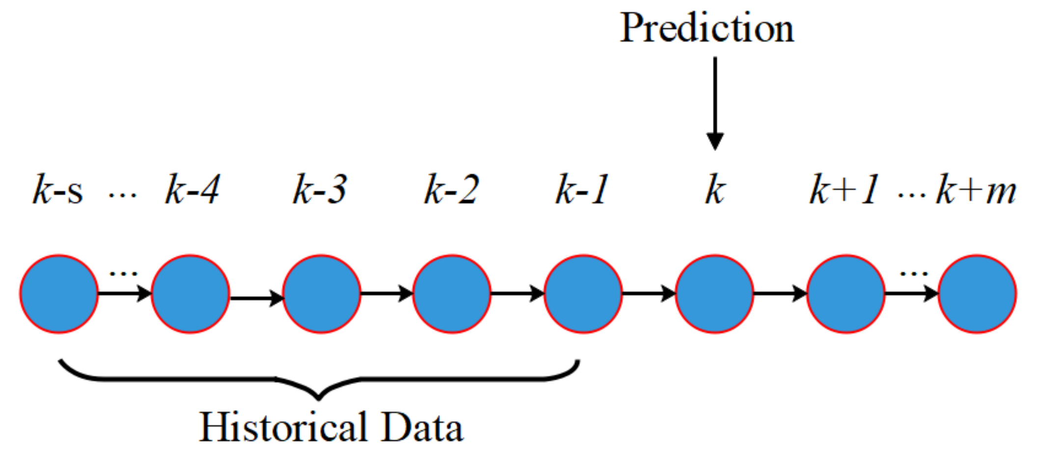
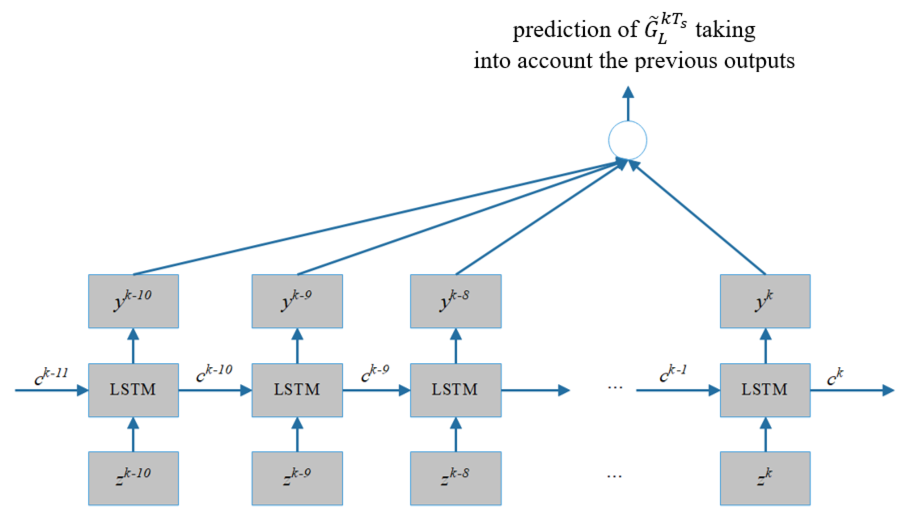
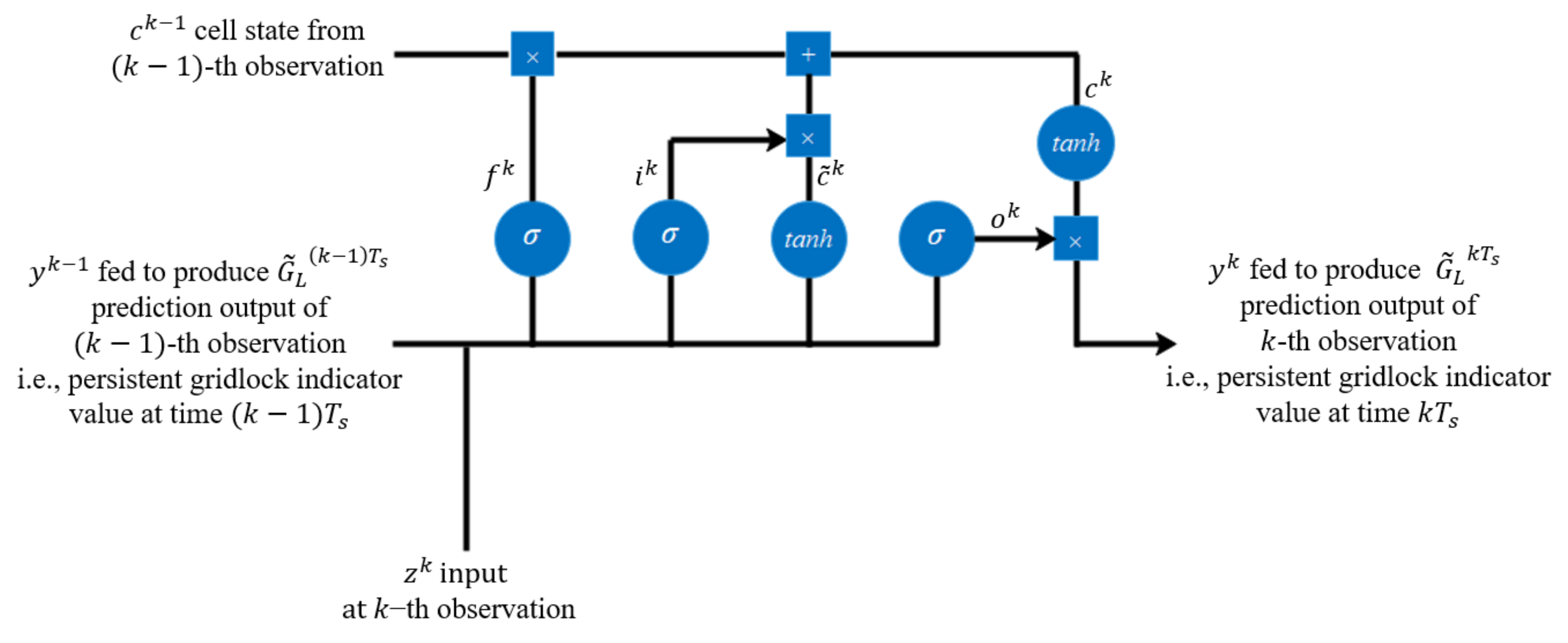
• This paper proposes gridlock prediction using temporal time series analysis based LSTM with time-lagged observations. This paper considers the lowest 1 min time-lagged observation period as a baseline to compare the prediction error values to study the effectiveness of LSTM on extended time-lagged observations.

The remainder of the paper is organized as follows. Section 2 provides the related works. Section 3 presents the simulation framework. Section 4 proposes the methodology of traffic data processing, the description of bottleneck and gridlock identification, and the study of sample sizes for gridlock detection. Section 5 presents the urban gridlock prediction based on the bottleneck with LSTM. Section 6 discusses the experimental results. Finally, concluding remarks are presented in Section 7.

2. Related Works

Traffic control and management are a primary issue in urban transport networks. In general, bottlenecks are identified and studied to find ways to overcome their negative effects on traffic. The traffic bottlenecks in urban road networks are more challenging to investigate than in freeways or simple arterial networks [8]. Traffic bottlenecks in urban road networks vary with traffic demands with spatiotemporal characteristics. Other events, such as traffic signals, traffic accidents, roadworks, and severe weather conditions, are required to consider more of their impacts on urban networks than in freeways.

When a bottleneck happens, there is a notable difference between traffic speed in the bottleneck area and its nearby downstream links. Oversaturation is usually caused by vehicle queues first occurring at some bottleneck intersections (i.e., critical intersections) and then propagating to neighboring upstream and downstream links between intersections. In [9], to identify oversaturated intersections, the authors proposed residual queue length estimation using shockwave speed. The authors also presented the detection of spill-over by identifying long detector occupancy time during the green phase. In [10], the authors proposed the identification of bottlenecks in an urban area practicing on causal congestion trees and graphs with the correlations of road segments according to the congestion propagation speed. More recently, in [11], the authors studied a traffic bottleneck identification method based on the traffic speed of loop detector data using the fusion of different collection cycles of loop detector data. To identify urban bottlenecks, in [1], the authors proposed a congestion analysis on the bottleneck core link and its neighboring links by clustering links based on the ranks of speed.

More recently, GPS-equipped vehicles were used in the field of bottleneck identification. In [12], the authors presented the processes of identifying and defining bottlenecks using GPS data obtained by trucks. In [13], the authors explored and identified bottlenecks in urban areas based on recurrent low-speed segments in the road network using GPS data. In [14,15], the authors used a spatiotemporal variation of speed to identify and classify bottlenecks using GPS data and crowdsourced traffic data. In [16], the authors tried to identify recurrent bottlenecks using spatial and temporal concepts on probe-reported speed data. In [17], the authors proposed a bottleneck identification method on urban expressways based on the traffic speed variance between the bottleneck area and its neighboring downstream links by analyzing the floating car data. In [18], the authors investigated traffic state and identified traffic bottlenecks on urban expressways using the fusion data accessible from fixed detectors and mobile navigation application data.

Future traffic condition prediction is a general concept [19]. In [20], the authors proposed the characterization of the traffic predictor to analyze vehicular traffic behavior for the different road segments using SUMO. In recent years, as deep learning techniques have advanced rapidly, researchers have started to adopt deep neural networks for high-accuracy traffic prediction. The Recurrent Neural Network (RNN) is widely known as a proper method to recognize the spatiotemporal evolution of traffic flow. In [21], the authors proposed a deep learning architecture based on the Recurrent Neural Network and Restricted Boltzmann Machine (RNN-RBM) to predict the spatiotemporal congestion evolution pattern using GPS data. In [22], the authors used an error-feedback Recurrent Convolutional Neural Network structure (eRCNN) for continuous traffic speed prediction. However, the traditional RNN fails to capture the long-term evolution. To resolve the vanishing gradient problem in RNN, a Long Short-Term Memory (LSTM) network was proposed in [23]. LSTM is well suited to classify, process, and predict time series given time lags of unknown duration. In [24], the authors proposed a novel short-term traffic volume prediction model using LSTM. More recently, in [25], the authors proposed a multiple time step short-term traffic prediction architecture using the RNN framework based on LSTM.

As mentioned above, the studies discussed identifying bottlenecks in intersections and respective upstream and downstream links in urban areas. Furthermore, LSTM has been applied in short-term traffic prediction. However, to the best of our knowledge, research on gridlock analysis has not yet been fully studied. We hope that this research will fill this gap by discussing the bottleneck and gridlock analysis based on the bottleneck at each intersection in the urban area. Congestion from the bottleneck originates traffic jams and propagates to neighboring upstream and downstream vicinities [26]. Such a situation usually leads to gridlock, which can potentially reduce traffic efficiency to an almost halted state, especially in a complex urban road network. 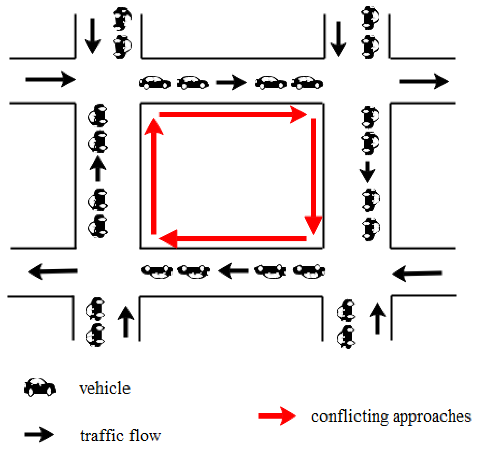Gridlock is used to describe severe road traffic congestion with zero flow [27,28]. Each interrelated intersection in a road network is fully occupied by slow-speed vehicles, and vehicles on conflicting approaches cannot move forward even when receiving a green traffic light, as shown in Figure 1. In our previous work [3], we proposed gridlock detection based on recurrent and non-recurrent congestion using the measurable gridlock characteristics in terms of traffic jam length and speed for both the upstream and downstream links of corresponding intersections. In previous work, we used simulated lane area detectors to detect gridlock, but these fixed-location detectors have some spacing limitations and installation costs in practice, as mentioned above.

3. Simulation Framework

Simulation models that can closely represent the real-world scenario are powerful and useful. In the area of road traffic simulation, three different models [29] are used, i.e., the (1) microscopic model, (2) macroscopic model, and (3) mesoscopic model. Microscopic simulation models have been used in several transportation areas in developing ITS technologies.

In this research, the Simulation of Urban MObility (SUMO) has been used to handle large, complicated road networks at a microscopic (vehicle-level) scale. SUMO is an open-source microscopic simulator developed by the German Aerospace Centre DLR in 2001 [30]. SUMO supports the traffic simulation community with a full-featured suite of modeling utilities, including the TraCI tool [31]. This tool is a Python API allowing users during the simulation run-time to retrieve simulated objects’ values, e.g., in accessing the speed of simulated GPS vehicles on each link in the simulated urban network.

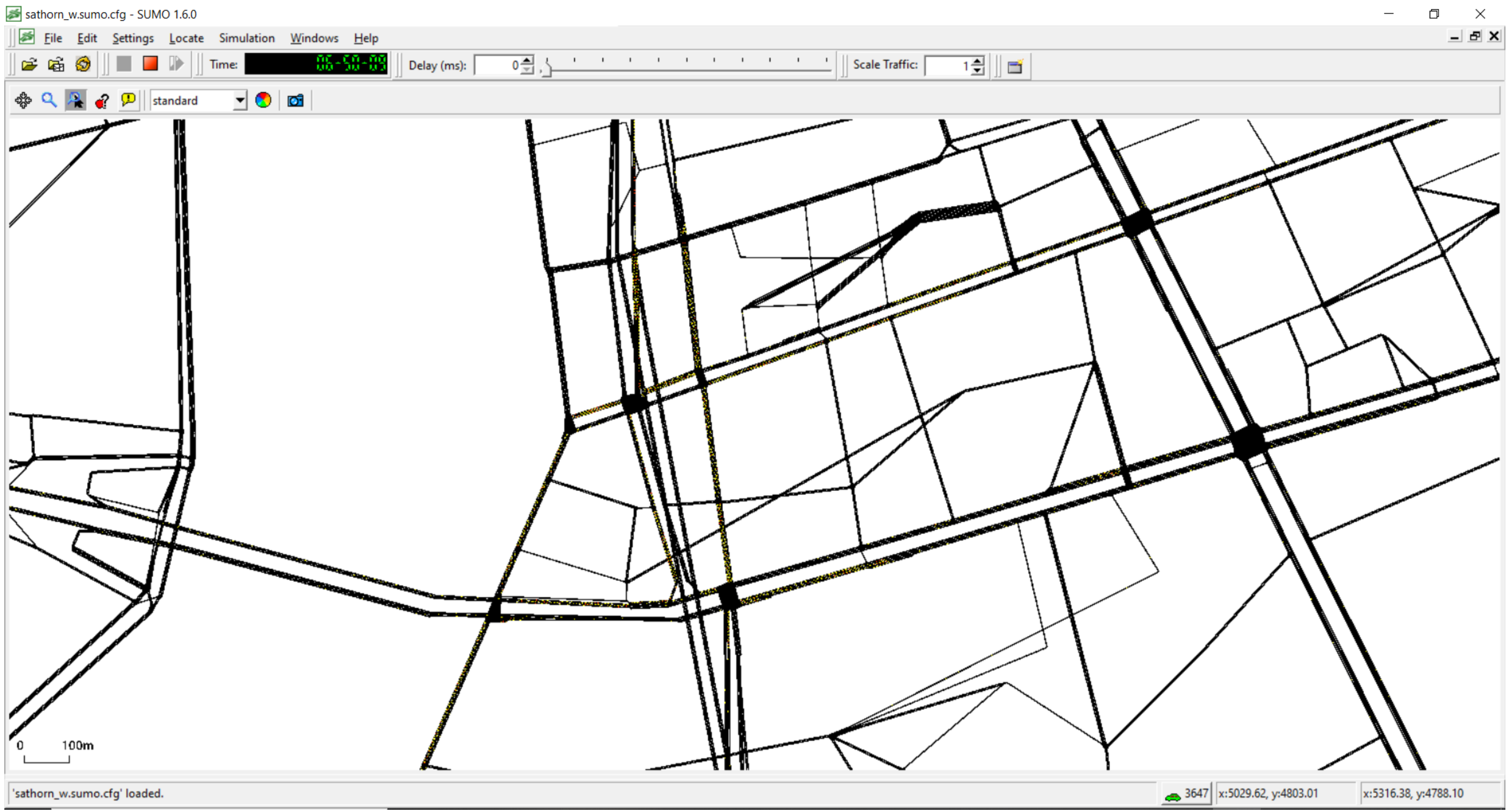
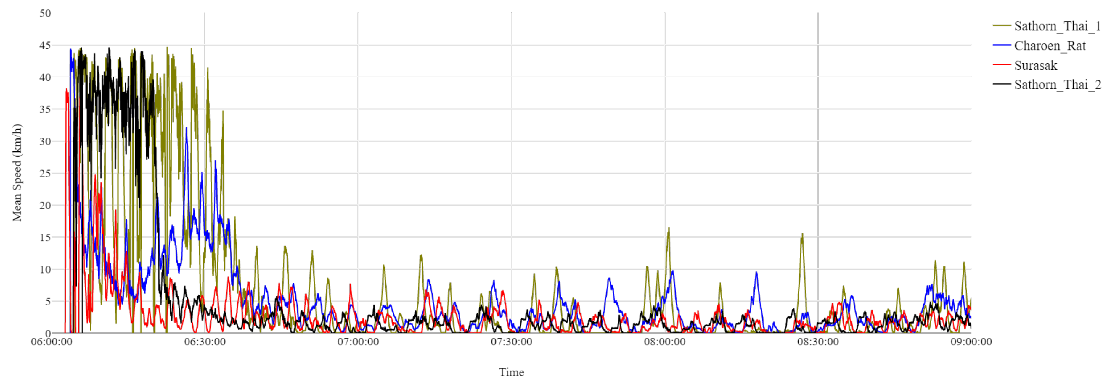
For traffic police and traffic engineer deployment, an educational tool [7] has been introduced by the Chulalongkorn University’s Sathorn Model project in Bangkok (Thailand), namely the Chula-Sathorn SUMO Simulator (Chula-SSS). By using this tool, traffic police can see the traffic signal phase, the queue length of vehicles in each upcoming direction at each signalized intersection, and the overall area with neighborhood road segments with user-friendly interfaces. Chula-SSS supports two calibrated datasets (morning and evening rush hours) for the Sathorn road network area. This study chose to investigate the morning case of Chula-SSS from 6 am to 9 am (corresponding to 21,600 s to 32,400 s after midnight). 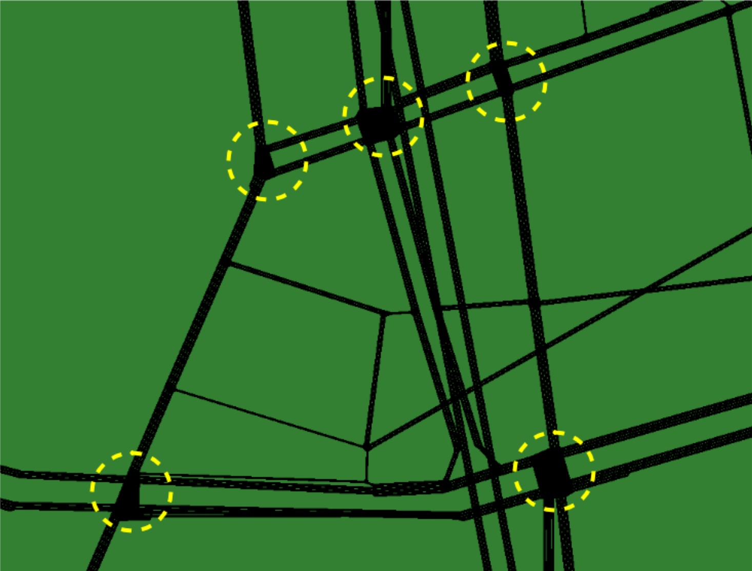This time interval is the morning congestion period during weekdays [7], whereby in practice, the local traffic police have often observed the real occurrences of gridlocks in the network. The simulated Chula-SSS consists of 2375 intersection nodes, 4517 edges, and 10 signalized intersections, as shown in Figure 2.

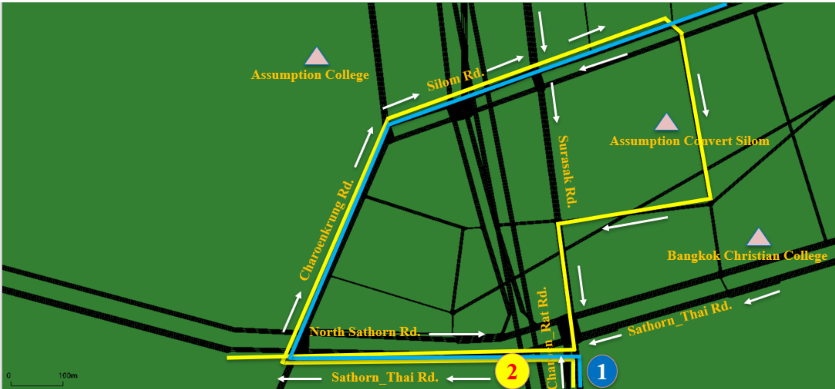
The dataset consists of 55,000 traveling vehicles in the morning or evening rush hours. Recurrent based gridlock happens on a daily basis in both morning and evening rush hours. This gridlock phenomenon has been intentionally disabled during the calibration attempt of Chula-SSS to find the optimal mobility model parameters. 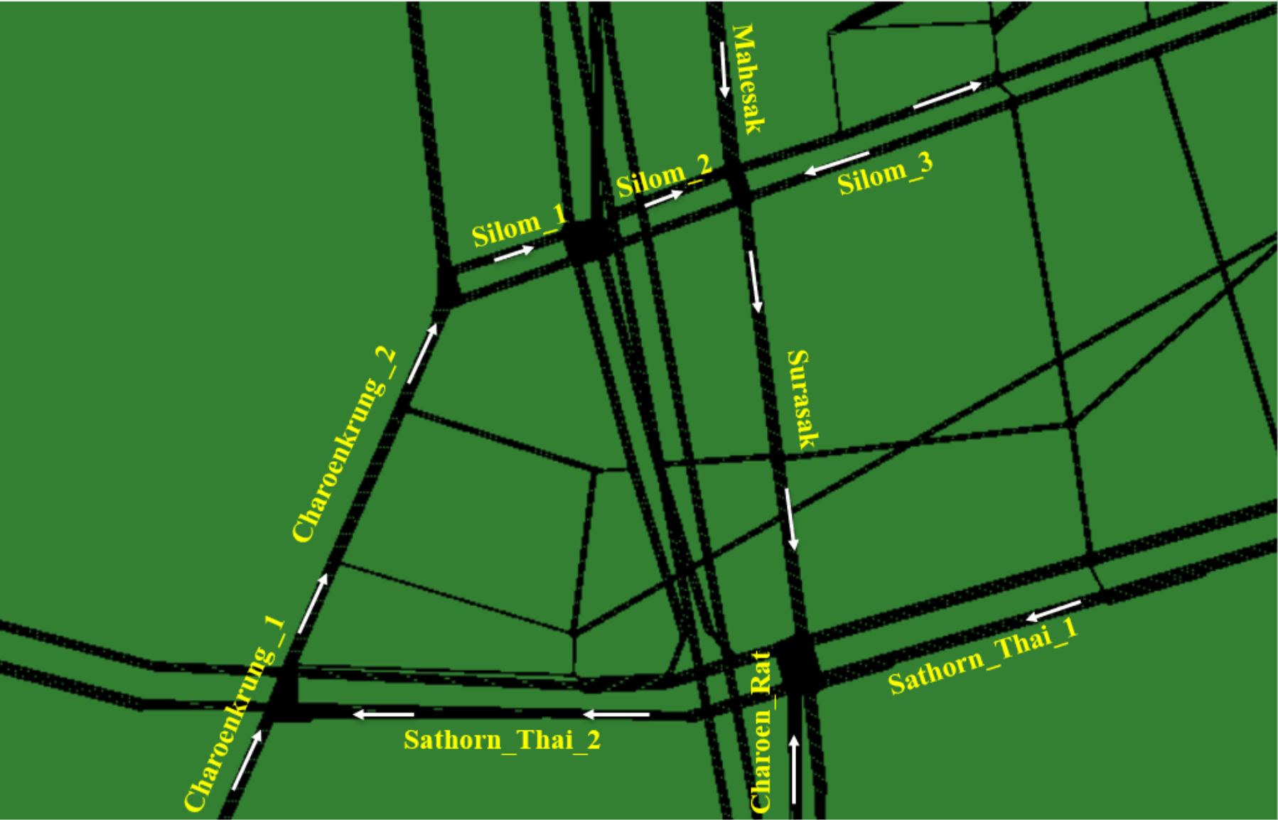To exhibit the case of gridlock during morning rush hours, the previous work [3] already included two extra routes (1 and 2) to the Sathorn critical region of Chula-SSS with traffic flows of 2125 vehicles (Route 1) and 1500 vehicles (Route 2) per hour, with their routes as shown in Figure 3. 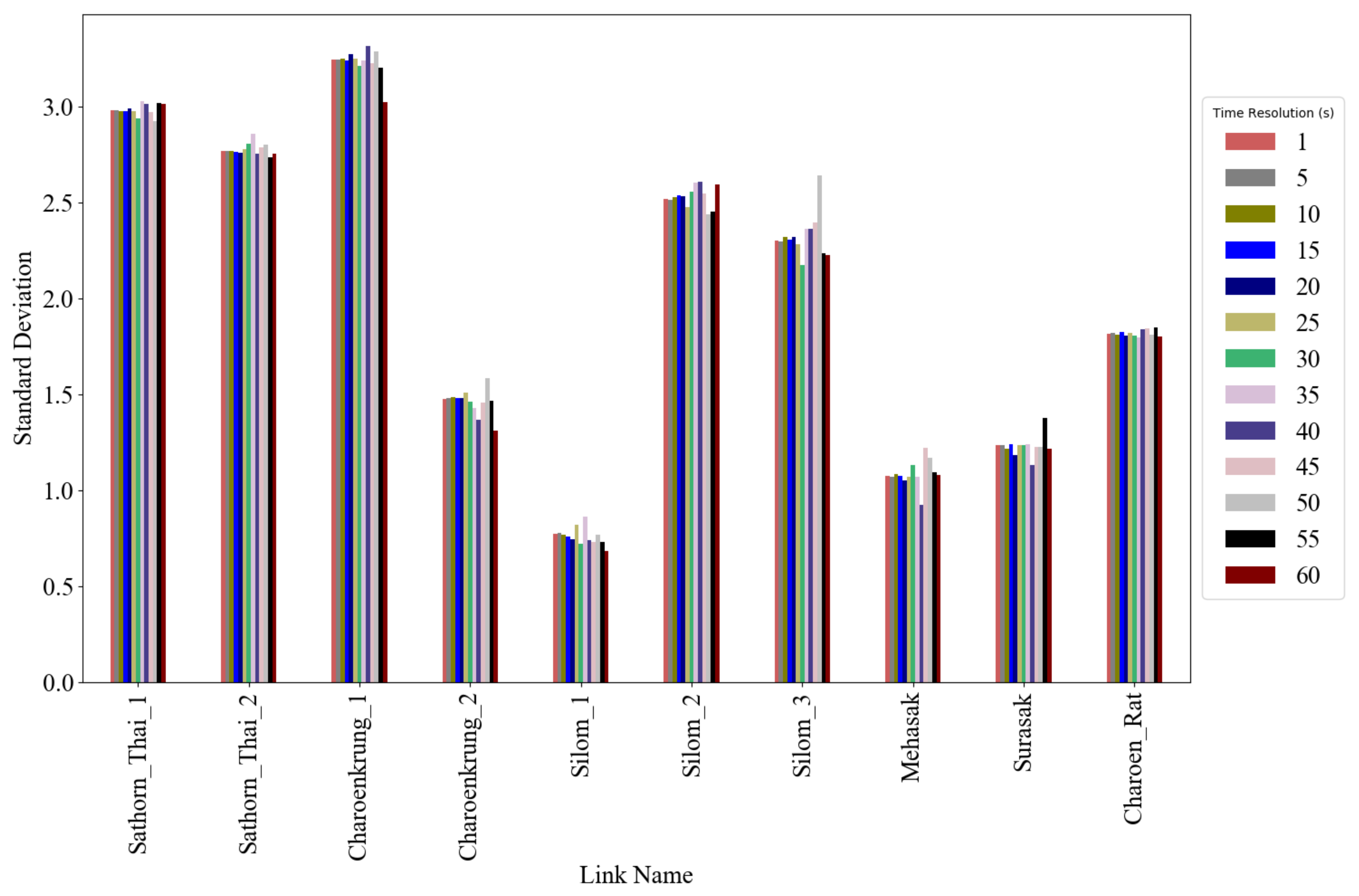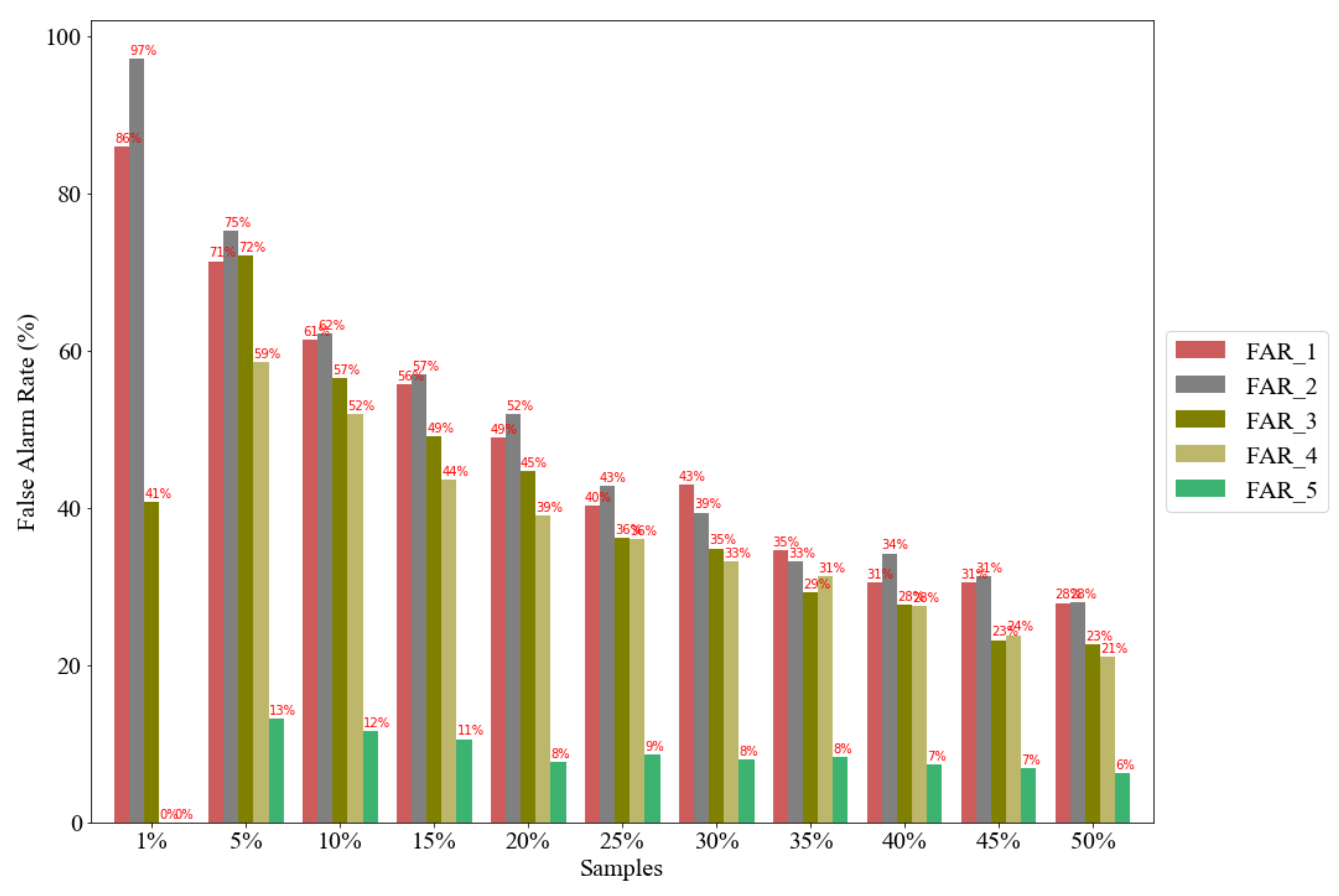The Sathorn critical region is where about 12,000 out of 55,000 vehicles travel on 10 edges, as shown in Figure 4. The GPS data collection has different time resolutions (1 s, 5 s, 10 s, 15 s, 20 s, 25 s, 30 s, 35 s, 40 s, 45 s, 50 s, 55 s, 60 s) within the simulation time interval for three hours from 6 am to 9 am. The collected vehicle data are assumed as GPS vehicles. With the limited penetration ratio of GPS vehicles, the different number of samples of GPS vehicles (1%, 5%, 10%, 15%, 20%, 25%, 30%, 35%, 40%, 45%, 50%) that passed through the links in the simulated gridlock area were investigated for the development of the identification of bottlenecks and the prediction of gridlock.

4. Methodology

4.1. Traffic Data Processing

A traffic network is comprised of a set of links and a set of junctions or intersections in the area of a typical urban transportation network. The network-wide congestion state of links is expressed as a $2\times 2$ matrix indexed in time (the number of time steps T) and space (the number of links N). Given the intersection and link topological characteristics, the intent is to develop a bottleneck identification for each intersection in the network using GPS vehicles as the input data. The initial step is to identify the traffic congestion state of each link using GPS data. The GPS data are collected with varying time resolutions (1 s, 5 s, 10 s, 15 s, 20 s, 25 s, 30 s, 35 s, 40 s, 45 s, 50 s, 55 s, 60 s) to represent the congestion state of each upstream link u and downstream link d, for each of the intersection areas. Herein, let e denote an arbitrary link index for upstream link u or downstream link d. The mean link speed $V_e^t$ of link e at time t is computed from the arithmetic mean of the speed values of all GPS vehicles on that link e at time t. In the matrix, the mean link speed $V_e^t$ values for all links e and time t is expressed as:

$$\left[\begin{array}{cccc}{V}_1^1& V_1^2& \cdots & V_1^T\\ \\ V_2^1& V_2^2& \cdots & V_2^T\\ ⋮& ⋮& \ddots & ⋮\\ V_N^1& V_N^2& \cdots & V_N^T\end{array}\right]$$

4.2. Description of Bottleneck and Gridlock Identification

In this study, the congestion state for each upstream link u and downstream link d is defined in terms of the low mean link speed indicator $C_e^t$ at time t of an arbitrary link e, as shown in Equation (1). The traffic congestion is set with the cut-off mean link speed threshold (5 km/h). If the mean link speed is less than or equal to the threshold, then the low mean link speed indicator $C_e^t$ of link e at time t is 1 (congested); otherwise, it is 0 (not congested).

$$C_e^t=\left\{\begin{array}{cc}1,\hfill & \mathrm{when}{V}_e^t<=5km/h\hfill \\ 0,\hfill & \mathrm{otherwise}\hfill \end{array}\right.$$

(1)

However, the low mean link speed for both the upstream and downstream can be affected by the red traffic signal light. To filter out such a red traffic signal light effect, therefore, if the low mean link speed indicator $C_e^t$ alerts that there is congestion for a long enough time interval of length w, then this congestion state is said to be persistent for the corresponding link. For instance, the time interval w is 10 min herein, which is long enough to filter out the usual red time intervals in practical scenarios in the Chula-SSS dataset [7]. The persistently low mean link speed indicator ${\tilde{C}}_e^t$ of link e at time t can then be expressed as:

$${\tilde{C}}_e^t=\prod _{\tau =0}^{w-1}{C}_e^{t-\tau }$$

(2)

A bottleneck occurrence at an intersection can be determined by considering two locations, upstream link u and downstream link d at the intersection. This study considers the direction of the upstream and downstream only on the conflicting approaches in the loop, as shown in Figure 1. A bottleneck is said to occur if and only if the low mean link speed indicator for any possible pair of upstream and downstream links at that intersection drops below a cut-off speed threshold. Let P be the number of upstream and downstream link pairs at intersection I, and ($u_j,d_j$) denotes the $j\mathrm{th}$ pair of upstream and downstream links, $(j=1,2,\cdots ,P)$. For intersection I, define the bottleneck indicator $B_I^t$ at time t as Equation (4) based on the low mean link speed indicators $C_u^t$ and $C_d^t$ for any upstream and downstream link pair ($u,d$) in I. If all pairs of upstream and downstream links of the intersection I are congested at t, then we say that there is a bottleneck in this intersection I at time t.

$$C_{(u,d)}^t=C_u^t·C_d^t$$

(3)

$$B_I^t=\prod _{\forall (u,d)\in \{(u_1,d_1),(u_2,d_2),\cdots ,(u_P,d_P)\}}{C}_{(u,d)}^t$$

(4)

A temporary low-speed intersection does not necessarily represent a bottleneck, but an active bottleneck always results in a low-speed intersection. Therefore, the persistent bottleneck indicator ${\tilde{B}}_I^t$ is used to confirm an active bottleneck for every time step $\tau$ within a time interval of length w, as shown in Equation (6).

$${\tilde{C}}_{(u,d)}^t={\tilde{C}}_u^t·{\tilde{C}}_d^t$$

(5)

$${{\tilde{B}}_I}^t=\prod _{\forall (u,d)\in \{(u_1,d_1),(u_2,d_2),\cdots ,(u_P,d_P)\}}\prod _{\tau =0}^{w-1}{\tilde{C}}_{(u,d)}^{t-\tau }$$

(6)

$$G_L^t=\sum _{I\in L}{B}_I^t$$

(7)

$${\tilde{G}}_L^t=\sum _{I\in L}{\tilde{B}}_I^t$$

(8)

With the bottleneck intersection identification, gridlock can be defined as the severe congestion state of a critical region that forms a loop of adjacent intersections in an urban road network. Let L be a set of potentially gridlock-looped intersections and $L=\{I_1,I_2,\cdots ,I_J\}$. For the Chula-SSS dataset, a recurrent gridlock loop is shown in Figure 5 with intersections within yellow dotted circles. The gridlock indicator for loop L, $G_L^t$, is triggered at time t if the bottleneck indicator $B_I^t$ for every intersection I ∈ L at time t is triggered, as shown in Equation (7). Consequently, the persistent gridlock is triggered due to the active bottleneck of all intersections, as shown in Equation (8). The computed gridlock labels quantizing the overall effect of the bottleneck indicators ${\tilde{B}}_I^t$ in loop L for all intersections are as shown in Figure 5. The computed gridlock labels are 0, 1, 2, 3, 4, and 5 based on the percentage of congested intersections in loop L. For example, if all intersections are not congested, then the computed gridlock label is 0; if 20% of intersections are congested, then the computed gridlock label is 1; if 40% of intersections are congested, then the computed gridlock label is 2, and so on, as shown in

Table 1. Gridlock labels.

Bottleneck Intersections	Gridlock Labels
all intersections are congested	5
80% of intersections are congested	4
60% of intersections are congested	3
40% of intersections are congested	2
20% of intersections are congested	1
all intersections are not congested	0

.

4.3. Effect of Sample Size on Gridlock Detection

The sample size selection is fundamental to any traffic engineering analysis, including bottleneck and gridlock analysis. Firstly, this section attempts to determine the time resolution based on the vehicles’ mean speed on the links in the interested area. The GPS data collection is simulated in the Chula-SSS dataset with different time resolutions (1 s, 5 s, 10 s, 15 s, 20 s, 25 s, 30 s, 35 s, 40 s, 45 s, 50 s, 55 s, 60 s) for the simulation time interval of three hours from 6 am to 9 am. Figure 6 shows the mean speed of all GPS vehicles on the upstream links (Sathorn_Thai_1, Charoen_Rat, Surasak) and downstream link (Sathorn_Thai_2) at the Surasak intersection. In this Figure 6, the mean speed of each upstream and downstream link reaches the congested conditions after the low mean speed. The standard deviation is the measure of the variability of the data distribution. Herein, the standard deviation of the mean speed of GPS vehicles on each upstream/downstream link for the sample size of 30% in each time resolution is shown in Figure 7. The reported results show that the standard deviation of the mean speed of all GPS vehicles on each upstream/downstream link obtained from 1 s at a high resolution is not statistically different from that obtained from 60 s at a low resolution. This suggests that any time resolution in the range of 1 s to 60 s can be used for bottleneck and gridlock analysis. Therefore, this study selected, for subsequent experimental investigations, the value of 60 s, which is currently available using GPS vehicles in practice for Bangkok’s targeted area in this research study.

Besides, this study investigated the sample size with which to experiment to analyze the status of gridlock with the multiple categories of gridlock labels based on bottleneck intersections. These gridlock labels are based on the identification of gridlock, as defined in Section 4.2. In particular, from the simulated movements of all GPS vehicles, we can compute the Detection Rate (DR) and the False Alarm Rate (FAR) of detected gridlock labels. DR and FAR are based on the True Positive (TP), True Negative (TN), False Positive (FP), and False Negative (FN) by:

$$DR=\left(\frac{TP}{TP+FN}\right)$$

(9)

$$FAR=\left(\frac{TN}{TN+FP}\right)$$

(10)

where TP, TN, FP, and FN measure the number of time steps for which corresponding results occur for the detection of gridlock label values. The detection of a gridlock label is said to be positive if, and only if, Equation (8) returns that gridlock label as the output. Otherwise, the detection is said to be negative for that gridlock label. The actual value of the gridlock label is computed by Equation (8) when 100% of simulated vehicles are assumed to have GPS data. In the case of less than 100% of available GPS data, the positive (or negative) detection results are said to be true or false according to whether or not the detection results are the same as those obtainable by the actual value of the gridlock label.

This section explores the effect of sample size on the identification of gridlock labels to understand the detection rate and false alarm rate. The detection rate and false alarm rate resulting from the settings of different sample percentages of GPS vehicles’ penetration ratio (1%, 5%, 10%, 15%, 20%, 25%, 30%, 35%, 40%, 45%, 50%) for the identification of gridlock labels are plotted in Figure 8 and Figure 9. Here, DR_1, DR_2, DR_3, DR_4, and DR_5 are indicated for the detection rate of the gridlock labels 1, 2, 3, 4, and 5. Furthermore, FAR_1, FAR_2, FAR_3, FAR_4, and FAR_5 are indicated for the false alarm rate of the gridlock labels 1, 2, 3, 4, and 5. These diagrams depict the detection rate and false alarm rate in each sample size with the time resolution of 60 s. In general, DR denotes the percentage of correctly detected gridlock. The algorithm works well in identifying gridlock labels if the DR is close to 100%. Notably, increasing the number of GPS vehicles will dramatically affect the detection rate and false alarm rate.

The data coverage of the road network is helpful for bottleneck and gridlock analysis. The higher the penetration ratio of vehicles with GPS in the road network is, the better the data coverage capability, and consequently, the detection rate increases and false alarm rate decreases, as shown in Figure 8 and Figure 9 for each gridlock label, except the sample size of 1% for low data coverage. Furthermore, it should be noted that the identification is most accurate for the gridlock label 5 (the network has been locked) in terms of both DR and FAR because the traffic flow of the gridlock-lopped intersections reaches almost the halted state. With the same logic for the explanation, on the contrary, identifying low gridlock labels (where the network is lightly or moderately loaded) is less accurate. However, such identification for lower gridlock labels poses less concern than when the whole network is gridlocked. Thus, a significant benefit of studying the detection rate and false alarm rate is that they allow for a means of gridlock prediction under the circumstances of the GPS vehicle penetration ratio. At the gridlock label 5, which is the most critical one for gridlock management, it is finally noted that to achieve the practical target of at least 80% DR and at most 10% FAR, Figure 8 and Figure 9 indicate that 30% of GPS vehicles are needed.

5. Urban Gridlock Prediction Based on Intersection Bottlenecks with Long Short-Term Memory

Time series modeling and prediction have been an active area of research due to the wide variety of applications [32]. Deep learning has been applied in time series analysis for both classification and prediction [33]. Prediction for time series is usually based on historical measurements. The better the learning of the inter-dependencies among past observations is modeled, the more accurate the prediction can be. Long Short-Term Memory (LSTM) [23] has been developed as an extension of the recurrent neural network with the advantages of learning long-range time dependencies.

5.1. Time Series Construction for Gridlock Prediction

The time series prediction methods have been developed over the years, advancing from simple regression techniques to statistical and intelligent algorithms. Short-term traffic flow prediction is a time series analysis that aims to predict traffic flow for a particular time based on historical traffic flow, as shown in Figure 10. This research adopted this concept to predict the severe road traffic congestion based on the historical time series congestion status of the intersections and gridlocks in the urban road network.

In our formulation, firstly, the time series observations of bottleneck indicators $B_{I_1}^t\dots ,B_{I_J}^t$ and computed gridlock indicator $G_L^t$ for each t are calculated. The values of all such indicators are then transformed to a multivariate time series of persistent bottleneck indicators for all intersections ${\tilde{B}}_{I_1}^t\dots ,{\tilde{B}}_{I_J}^t$ and computed persistent gridlock indicator ${\tilde{G}}_L^t$, as defined earlier in Section 4.2. A multivariate time series is denoted as $X=〈{\tilde{B}}_{I_1}^T\dots ,{\tilde{B}}_{I_J}^T,{\tilde{G}}_L^T〉$ with time stamp T. To take into account all the intersections that can form a potential gridlock loop, define $x^t$ as the vector of all persistent bottleneck indicators of ${\tilde{B}}_{I_1}^t\dots ,{\tilde{B}}_{I_J}^t$ and persistent gridlock indicator ${\tilde{G}}_L^t$ for each t, as shown in

Table 2. Observation instances of observed and computed time series.

Instance	Bottleneck						Gridlock
$x^1$	${\tilde{B}}_{I_1}^1$	${\tilde{B}}_{I_2}^1$	.	.	.	${\tilde{B}}_{I_J}^1$	${\tilde{G}}_L^1$
$x^2$	${\tilde{B}}_{I_1}^2$	${\tilde{B}}_{I_2}^2$	.	.	.	${\tilde{B}}_{I_J}^2$	${\tilde{G}}_L^2$
$x^3$	${\tilde{B}}_{I_1}^3$	${\tilde{B}}_{I_2}^3$	.	.	.	${\tilde{B}}_{I_J}^3$	${\tilde{G}}_L^3$
⋮	⋮	⋮	⋮	⋮	⋮	⋮	⋮
$x^T$	${\tilde{B}}_{I_1}^T$	${\tilde{B}}_{I_2}^T$	.	.	.	${\tilde{B}}_{I_J}^T$	${\tilde{G}}_L^T$

. As indicated in Figure 10, to distinguish the time instances used in simulating detailed system dynamics and in obtaining the time series observations with the potentially more extended time sampling period, we change the previously used time indices from t to k for the following gridlock prediction formulation.

Define the k-th observation value as the original time series value sampled at time $t=k{T}_s$ where $T_s$ denotes the length of the time sampling interval. The basic idea in this study is to predict the k-th observation $y^k$ fed to produce ${\tilde{G}}_L^{k{T}_s}$ from a finite set of s time-lagged observations; we aim at predicting in a rolling forecasting fashion, herein defined as:

$$\begin{array}{c}\hfill \begin{array}{c}\hfill z^k=\{x^{(k-1)T_s},\dots ,x^{(k-s)T_s}\}\end{array}\end{array}$$

(11)

where $x^{(k-1)T_s},\dots ,x^{(k-s)T_s}$ denote the corresponding time sampled values for the k-th observation. The input historical bottleneck and computed gridlock sequence are used to predict gridlock at the k-th observation. Figure 11 shows the unrolled network of time-lagged observation to predict $y^k$ over the set of time-lagged observations $z^k$. In the experiments, we consider $z^k=x^{(k-1)T_s}$, i.e., $s=1$ for the case of using one time-lagged observation, as well as trying to increase s, the number of time-lagged observations.

5.2. Formulation for the Prediction of the Time Sampled Persistent Gridlock Indicator

The LSTM has the advantage of capturing temporal information and is approved to be adopted in time series modeling. It is a special kind of recurrent neural network with a purpose-built memory cell representing long-term dependencies in the time series data.

The memory cell has three units, namely the input gate ($i^k$), the forget gate ($f^k$), and the output gate ($o^k$), to maintain the information of a long period. The forget gate determines what information is required to be rejected from the input $z^k$. The input gate $i^k$ determines what information $z^k$ is required to be kept, and the output gate $o^k$ produces the output based on $z^k$. They are composed of a sigmoid neural network layer ($\sigma$), pointwise multiplication operation, and tanh function, as depicted in Figure 12. $w_f$, $b_f$, $w_i$, $b_i$, $w_o$, and $b_o$ are the weight matrices and bias vectors of each gate. The gates are updated in LSTM by [23]:

$$\begin{array}{cc}\hfill f^k& =\sigma (w_f·[z^k,y^{k-1}]+b_f)\hfill \\ \hfill i^k& =\sigma (w_i·[z^k,y^{k-1}]+b_i)\hfill \\ \hfill o^k& =\sigma (w_o·[z^k,y^{k-1}]+b_o)\hfill \end{array}$$

(12)

After updating the gates, the updated values from the input and forget gates are used for updating the current state $c^k$ of the LSTM unit based on ${\tilde{c}}^k$ and $c^{k-1}$·$w_c$ and $b_c$ are the weight metrics and bias vector, and tanh is the activation function. The output $y^k$ is triggered by the output gate $o^k$ as defined in Equation (13), which yields the activated output to the next LSTM unit.

$$\begin{array}{cc}\hfill {\tilde{c}}^k& =tanh(w_c·[z^k,y^{k-1}]+b_c)\hfill \\ \hfill c^k& =f^k·c^{k-1}+i^k·{\tilde{c}}^k\hfill \\ \hfill y^k& =o^k·tanh\left(c^k\right)\hfill \end{array}$$

(13)

Additionally, the activation sigmoid function $\sigma$ is used to map the range of [0,1], and the tanh function is applied to map the range of [−1,1].

6. Evaluation of the LSTM Based Prediction Experiment on the Chula-SSS Dataset

This study used a dataset that has been collected from the GPS vehicles sampled from the calibrated Chula-SSS dataset in SUMO using different random seed numbers for a total of 100 simulated days (each from 6 am to 9 am). The GPS data collection was periodically sampled every 60 s during the simulation time interval. To develop and evaluate the LSTM model, the dataset was divided into training data containing 80 simulated days and testing data containing the remaining 20 simulated days from a total of 100 simulated days. Each simulated day has 181 time steps (every 60 s within 6 am to 9 am) and 6 features by combining the 5 persistent bottleneck indicators of 5 intersections and 1 persistent gridlock indicator. The important step is to select the model hyperparameters. In this investigation, the hyperparameters of LSTM include the number of neurons to improve the network’s learning capacity, the number of epochs, and the batch size, as shown in

Table 3. Description of the LSTM model setup.

Item	Description
Prediction Target	Gridlock labels (0, 1, 2, 3, 4, 5)
Input Variable	Multivariate time series observations for all intersections
Training Parameters	epochs, number of neurons, batch size

. The number of epochs defines the number of times that the learning algorithm will work through the all training data. The models were developed with the standard Keras library [34]. Additionally, the standard gradient descent algorithm, ADAM [35], was used to update the weight values given the batch size value.

To evaluate the effectiveness of the gridlock prediction model, we calculate the Root Mean Squared Error (RMSE) and Mean Absolute Error (MAE) [36] in estimating the time sampled values of the persistent gridlock indicator. These metrics are calculated by comparing the time series’s target values and the corresponding time series for the concatenation of all the testing data, each lasting for three hours. The proposed approach for predicting time series is applied to predict gridlock based on the bottleneck state for each intersection in the experiments with different sample sizes by varying the GPS vehicle penetration ratio in percentage and with various settings on the time-lagged observation period ($s{T}_s$) and the time sampling interval $\left(T_s\right)$. 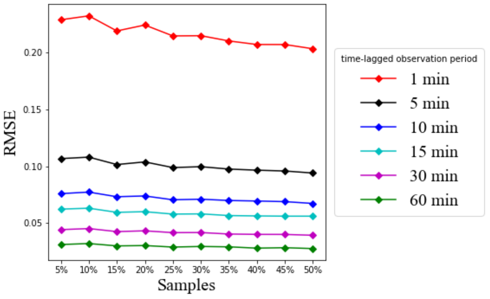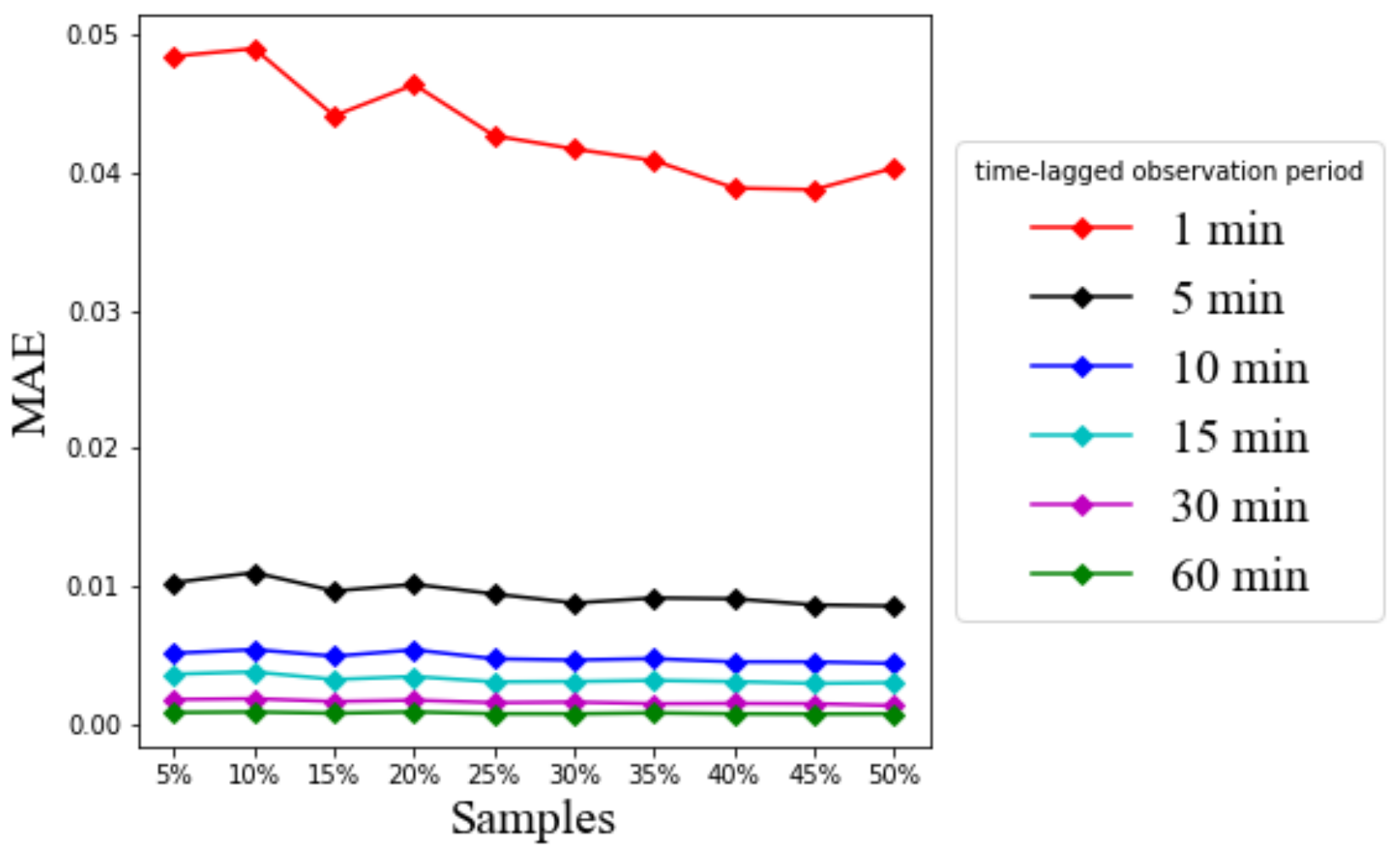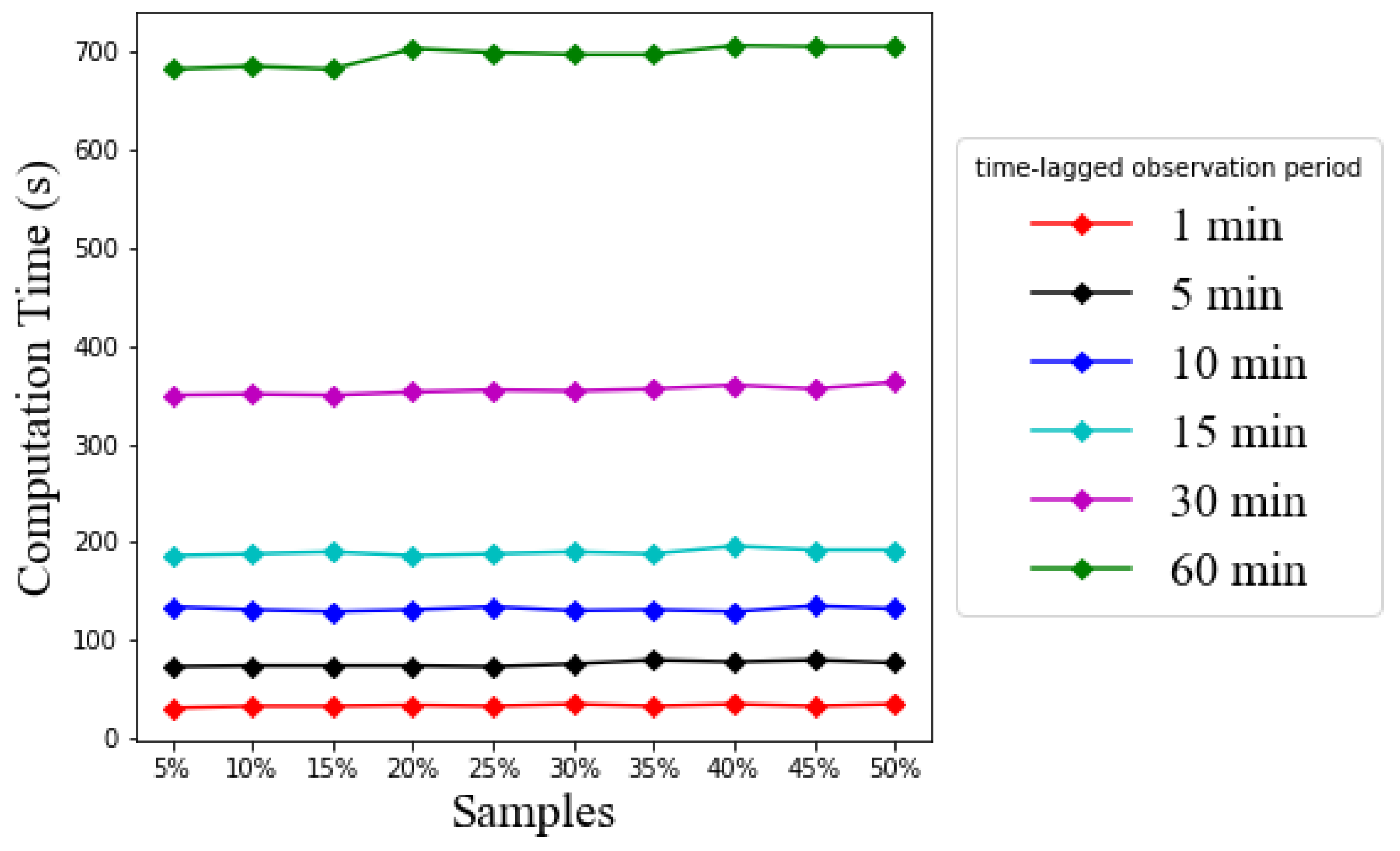Figure 13, Figure 14 and Figure 15 report the obtained results, i.e., the RMSE and the MAE, as well as the required computation time of LSTM.

6.1. Effect of Time-Lagged Observation Period

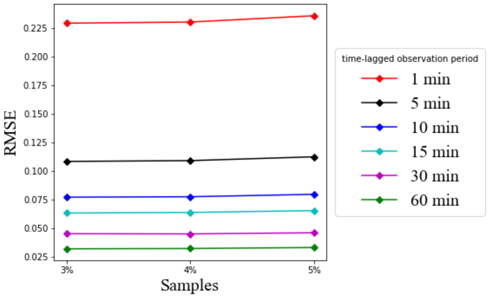
Firstly, the time-lagged observation period ($s{T}_s$) was varied as 1, 5, 10, 15, 30, and 60 min, as shown in Figure 13, Figure 14 and Figure 15. Herein, the time sampling interval ($T_s$) for every 60 s was used. Figure 13 shows the RMSE values for different time-lagged observation periods using 10 neurons of LSTM outputs linearly combined with the final dense layer with one prediction output, 10 epochs, and a batch size of 50. 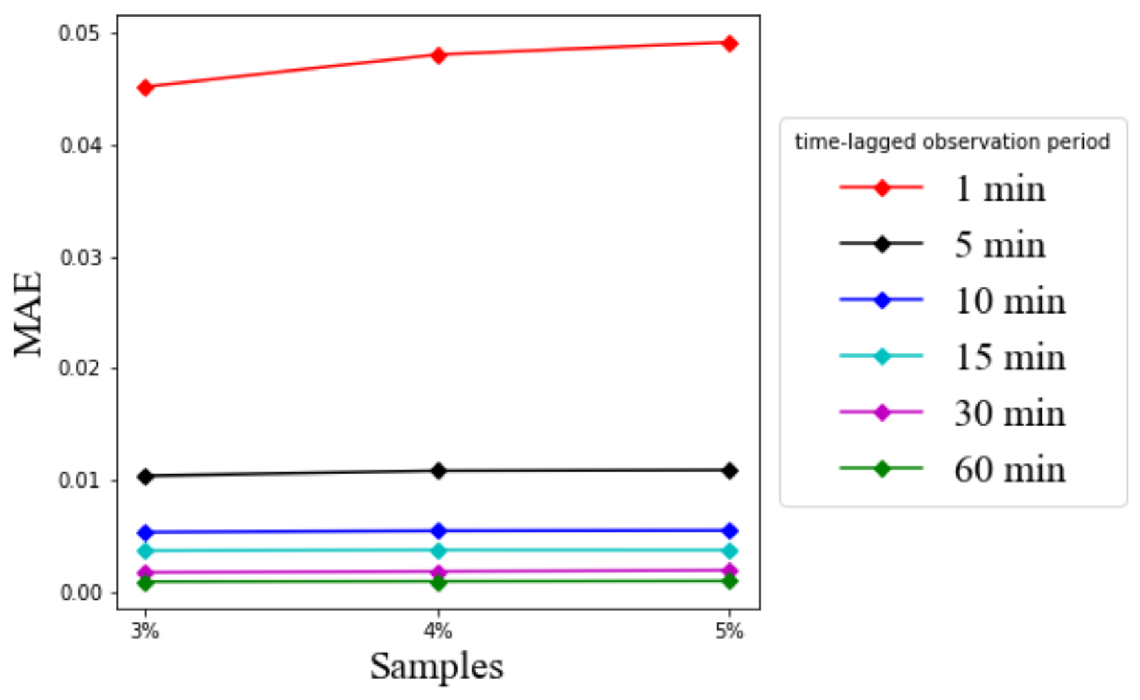Figure 14 shows the MAE values for different time-lagged observation periods using the same parameters. These hyperparameter values were searched by brute force and finally selected to show the achieved performance of LSTM in our considered case studies. To compare the prediction error values, this study considered as a baseline the lowest 1 min time-lagged observation period, i.e., LSTM is allowed to look back into the past for only 1 min. Figure 13 and Figure 14 show that the RMSE and MAE eventually decrease with the increase of the past observation interval length allowable for LSTM based prediction. When the time-lagged observation is 1 min, there is a big gap between the RMSE values and the other time-lagged observations of 5 min to 60 min. It is understandable that the short historical observation interval cannot provide adequate information for accurate prediction. However, the gap of the RMSE and MAE values between 5 min and other time-lagged observation periods from 10 min to 60 min is relatively not as much as that from 1 min to 5 min.

Although a short historical observation interval does not generally provide accurate prediction, Figure 13 and Figure 14 suggest that the RMSE and MAE values are still acceptable even at the 1 min time-lagged observation, i.e., less than 0.25 for RMSE and 0.05 for MAE from the presumed linear scale of five. On the other hand, if LSTM has more information on the extended time-lagged observation, the RMSE value is reducible to as low as 0.02, and the MAE value is as low as 0.001 with the 60 min time-lagged observation. Therefore, the result confirms that LSTM has good performance over the whole practical range of time-lagged observations. The performance improves further when the input time-lagged observations are sufficiently long.

Although prediction accuracy is improved, if the number of time-lagged observations is increased, the computation is unavoidably increased, as shown in Figure 15. The computation time reported here is based on the currently used hardware of NVIDIA GeForce GTX 1080 Ti with 11 GB memory. At the 60 min time-lagged observation period, it is found that the computation time is up to 700 s or almost 12 min. Such a computation time can be further reduced if the hardware capacity is upgraded. In practice, engineers can design the needed hardware so that the computation can be completed within the time sampling interval, resulting in a real-time prediction effect.

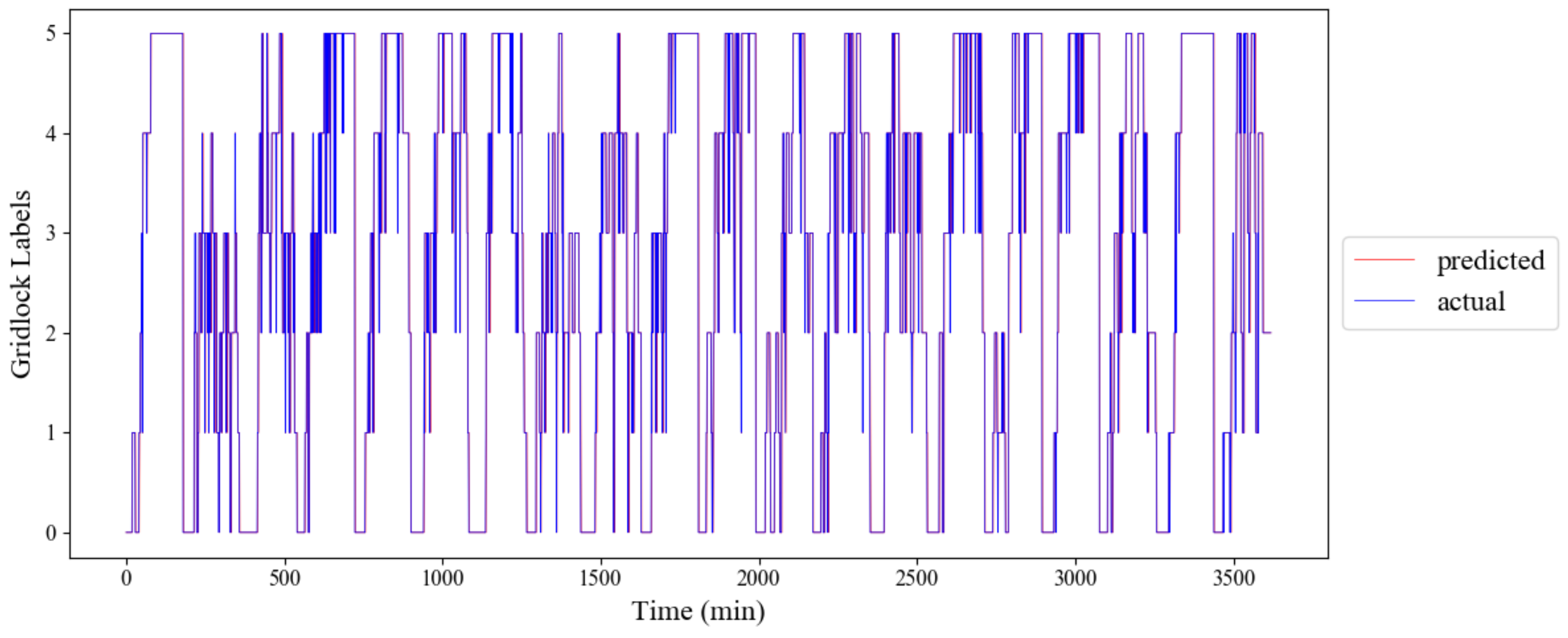
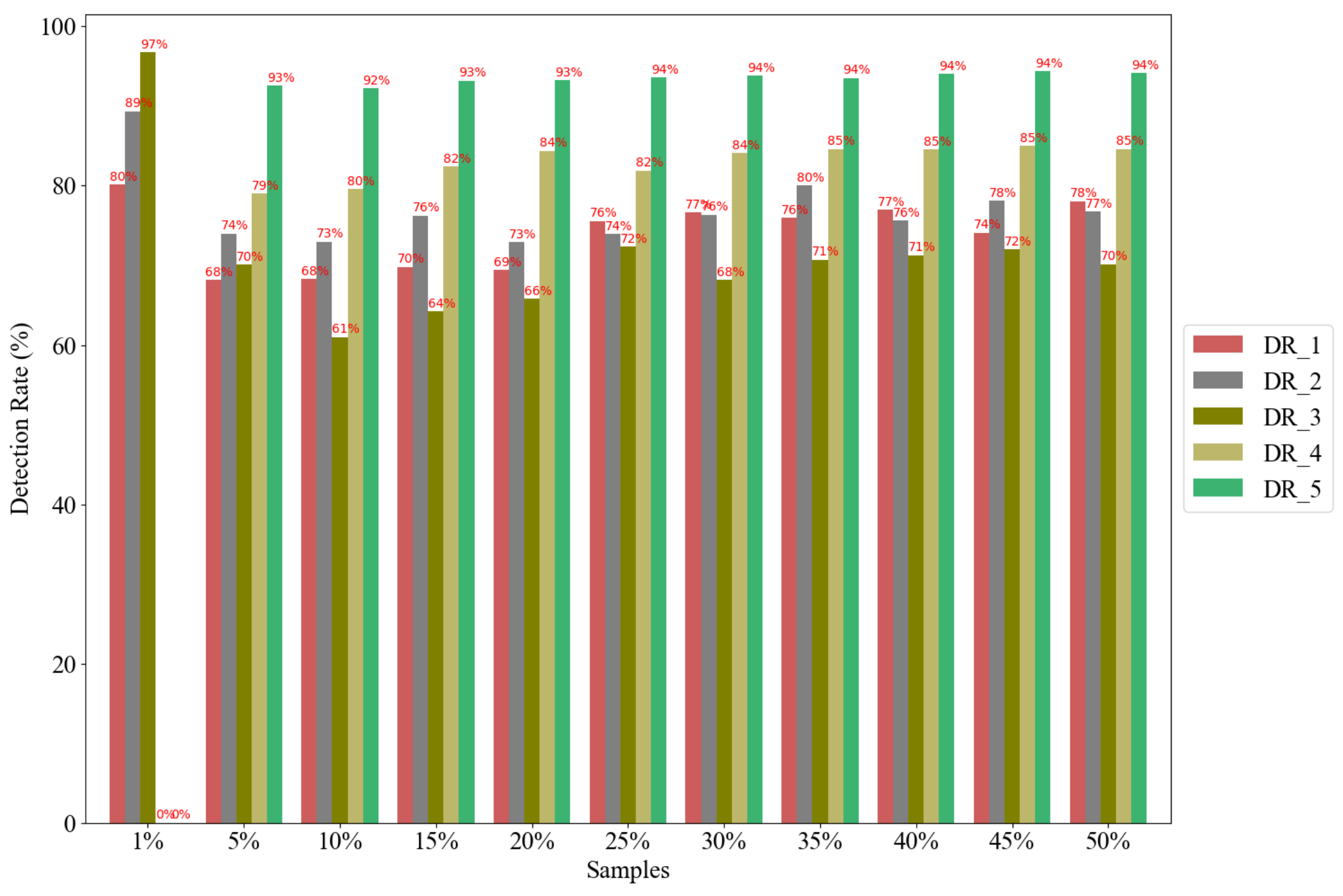
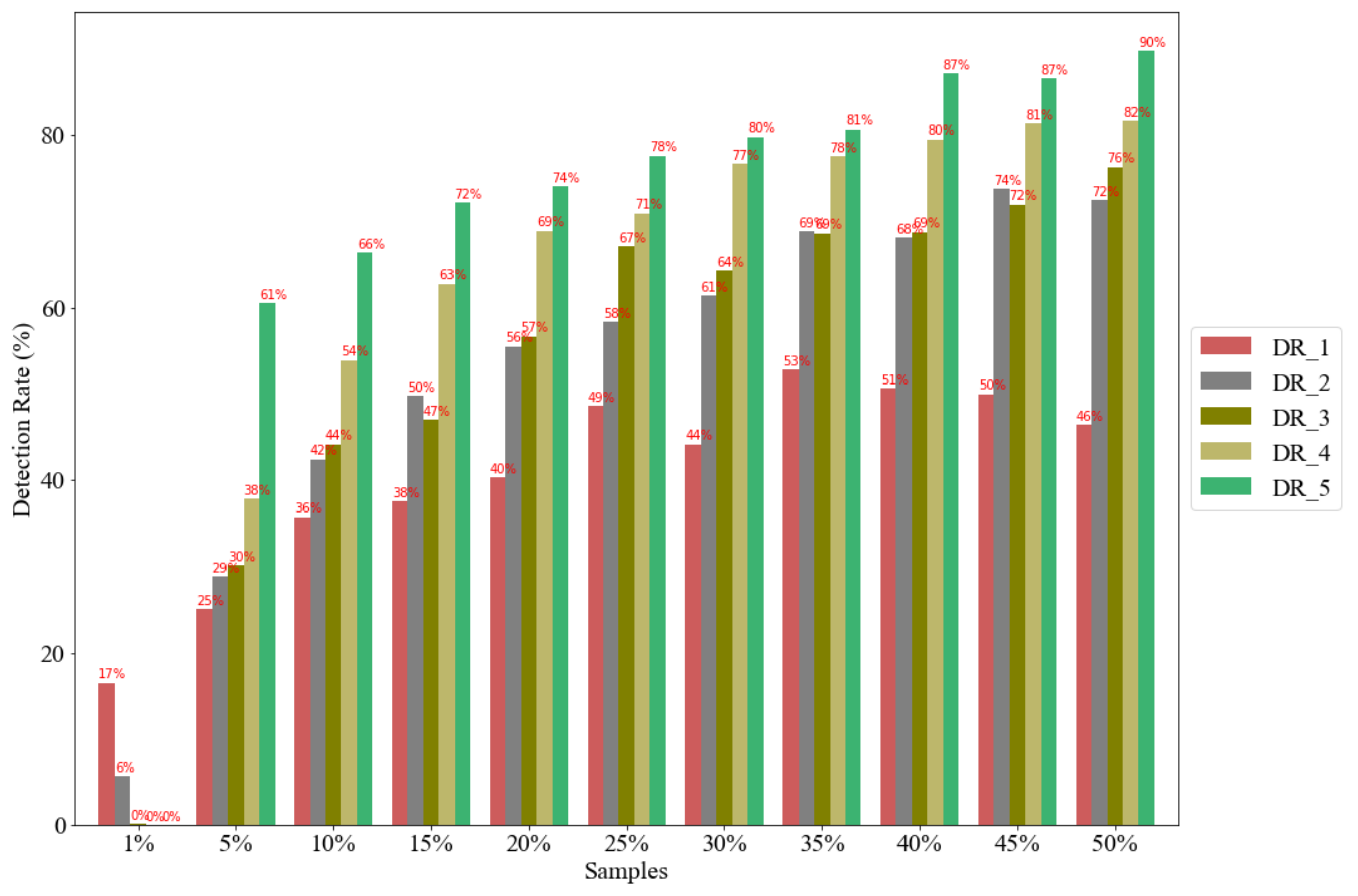
Figure 16 shows the predicted and actual gridlock labels with 1 min time-lagged observation using the 5% sample size. Figure 17 shows the detection rate for all gridlock labels after prediction with LSTM. In Section 4.3, this study presents the effect of sample size to detect gridlock, and the detection rate is 80% on the sample size of 30% GPS vehicles. However, after prediction with LSTM, our proposed LSTM model can predict more gridlock labels, 1, 2, and 3, as low as the 1% sample, but the 1% sample cannot predict the gridlock labels 4 and 5 using the insufficient information of the loop. In Figure 17, the reported DR is 93% for the 5% sample size. This reported detection rate after LSTM confirms that LSTM has good performance using the time-lagged observation in the rolling forecast fashion.

In Figure 18 and Figure 19, the reported RMSE and MAE values are decreased to as low as 0.03 and 0.001 with the 60 min time-lagged observation using the 3% sample. Therefore, the results confirm that the required minimum sample size of 3% GPS vehicles traveling on each link of the loop is enough to predict the gridlock. Using the mean speed of this penetration ratio of GPS vehicles, in practice, can successfully and effectively detect gridlock.

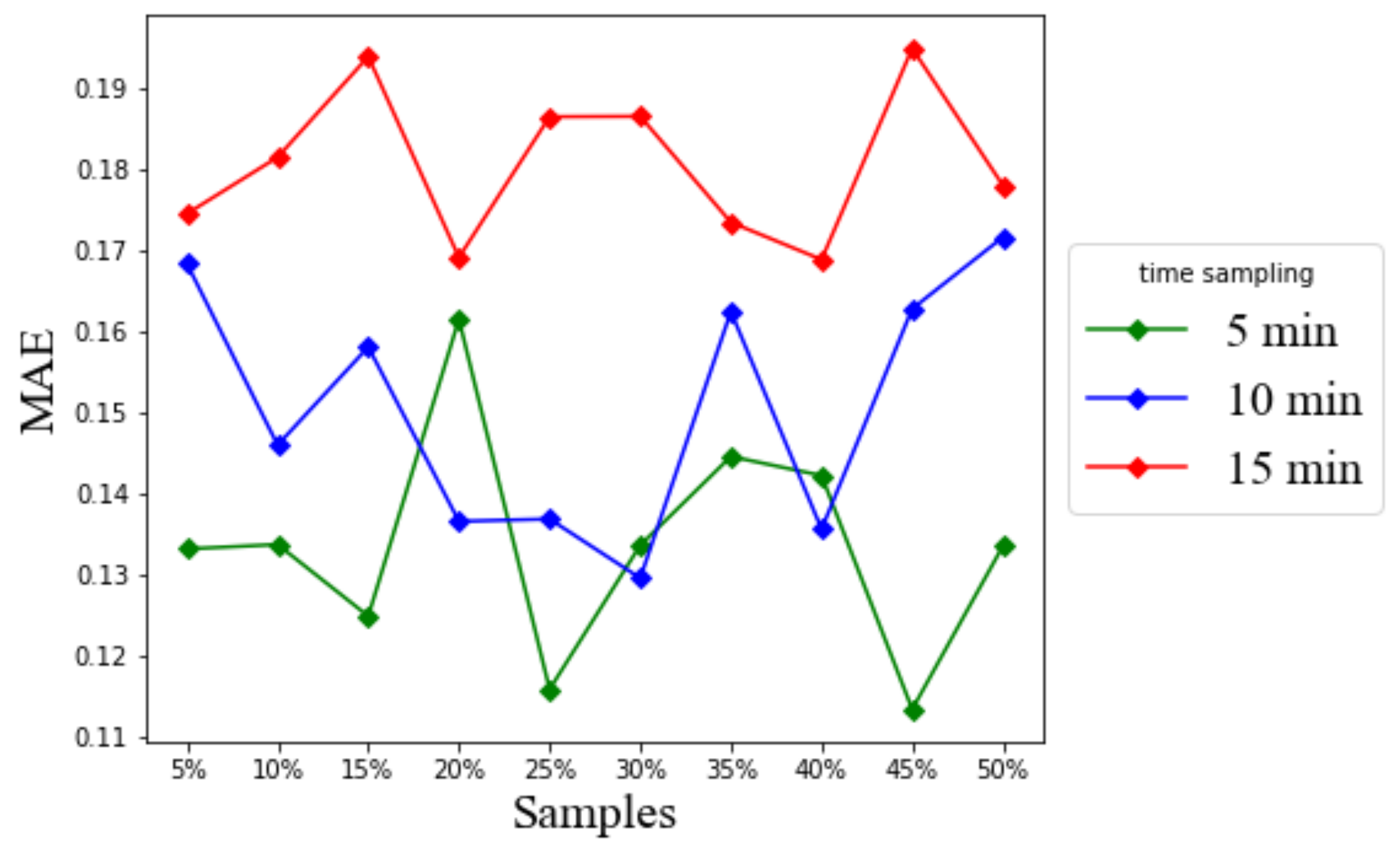
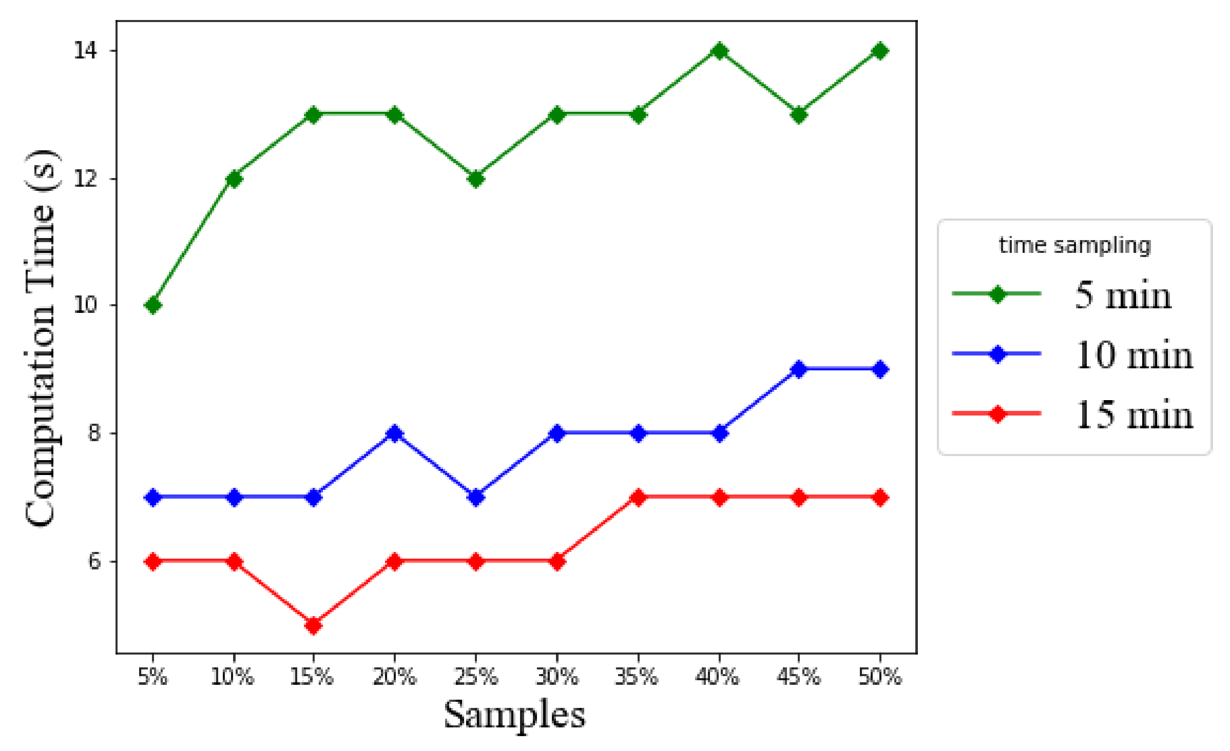
6.2. Effect of Time-Sampling

A short time sampling interval of data collection refers to a high sampling rate, while a long time sampling interval of data collection refers to a low sampling rate. The higher sampling rate of GPS vehicle trajectories gives more sampling points to form the trajectory path. However, because of the strict limits of battery storage for hand-held GPS-embedded devices carried inside moving vehicles, they are often unable to collect high sampling rate data for a long period [37]. Therefore, the time sampling rate interval of GPS vehicle data is an important issue. To study the effect of the sampling interval in gridlock prediction, this study used the time sampling interval $T_s$ of the GPS vehicle data in Figure 20, Figure 21 and Figure 22 at 5, 10, and 15 min. Like in Figure 13, Figure 14 and Figure 15, we selected the LSTM hyperparameter values of 10 neurons, 10 epochs, and a batch size of 50.

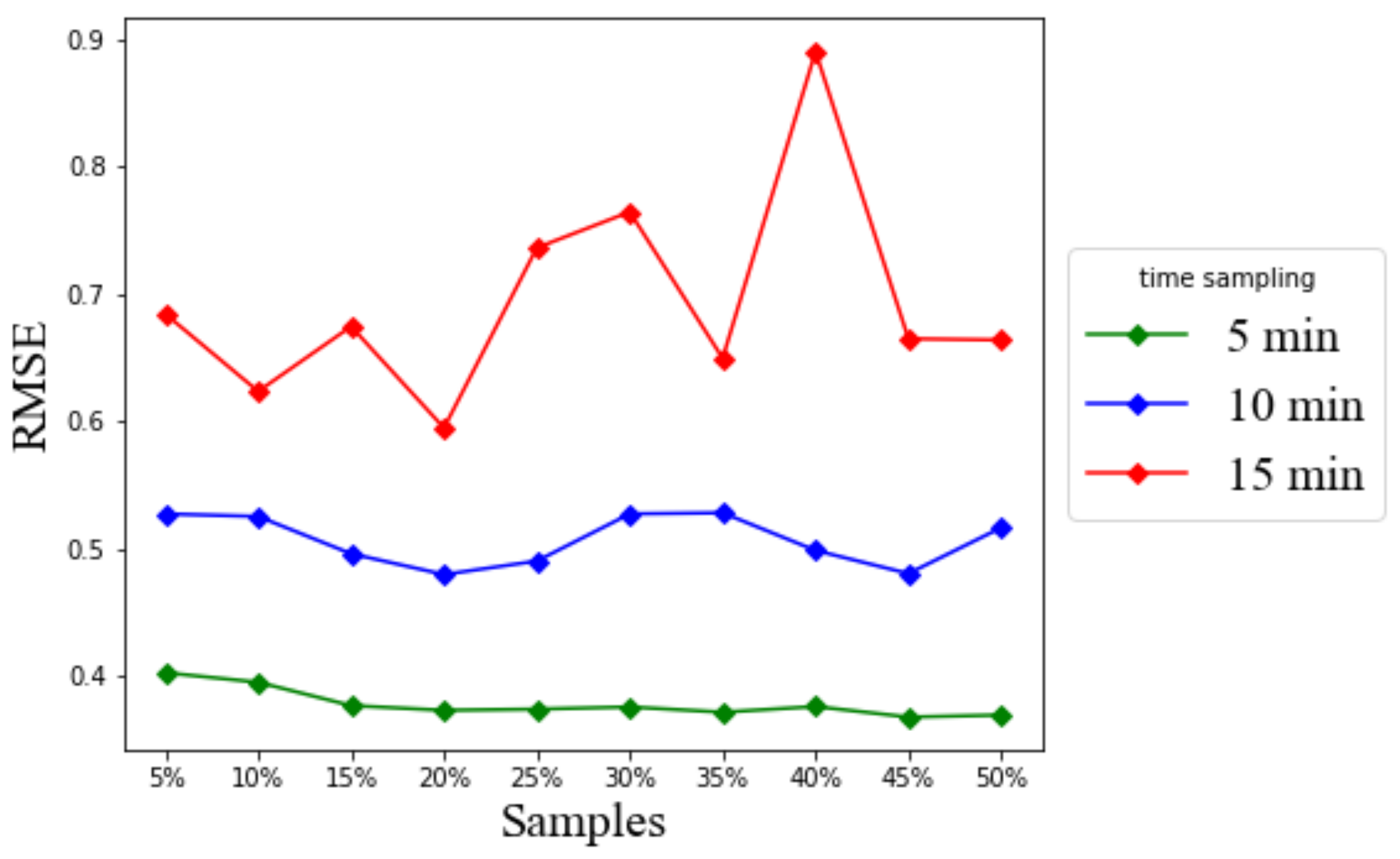
Our findings suggest that the time sampling interval directly affects the achievable accuracy of LSTM prediction for persistent gridlock indicators. In Figure 20, the reported prediction error increases as the time sampling interval increases. The prediction error obtained from the time sampling interval of 5 min is at most 0.4 for RMSE for the minimally required 5% GPS vehicle sample. However, a long time sampling interval results in a large RMSE value, for example up to 0.9 for RMSE for the 15 min time sampling. From the computation time point of view, the longer the time sampling interval, the less the computation time, as shown in Figure 22. For example, the 15 min time sampling lasts only around 6 s or 7 s.

In practice, one can evaluate the quantized gridlock label by rounding off the predicted gridlock label value first. In this case, an RMSE less than 0.5 should be considered as acceptable. Under such practical concerns, based on Figure 20, Figure 21 and Figure 22, the proposed LSTM based model can predict the gridlock label for effectively 5 min into the future and at the affordable up to 15 s computation time. That lead time of 5 min is comparable to a reasonable cycle length of adjusting traffic signal lights. Therefore, by foreseeing such gridlock occurrences by one control cycle, at least, the operational traffic signal controller can adaptively try to correct its signal interval settings to either mitigate the occurring gridlock effects or prevent the gridlock from happening in the first place.

7. Conclusions

This study proposes bottleneck based gridlock prediction on simulated GPS vehicles using spatiotemporal time series analysis based LSTM. The investigation shows that LSTM can predict the gridlocks with a long range of time dependencies by conducting the experiments on different time-lagged observation periods and time sampling. The sample size of 30% GPS vehicles is needed for geographic data coverage of bottleneck and gridlock analysis before using LSTM. The RMSE result of 0.02 with the 60 min time-lagged observation confirms that LSTM prediction with current hardware capacity has satisfying performance if the input time-lagged observations are sufficiently long. The time sampling interval of 5 min reports 0.4 for RMSE with the required sample of 5% GPS vehicles. The reported results suggest the effect of time sampling using the data collection interval of 5 min. Our proposed LSTM model can predict the gridlock labels for effectively 5 min into the future with a 15 s computation time. Therefore, if our LSTM model has information on the previous time-lagged observation of a 5 min data collection interval, it can predict the future 5 min of the gridlock occurrences. The traffic signal controller can adapt to correct the signal timings to alleviate the gridlock effects in the loop. The reported RMSE and MAE values are decreased to as low as 0.03 and 0.001, with the 60 min time-lagged observation using the 3% sample with LSTM. Therefore, the results confirm that the required minimum sample size of 3% GPS vehicles traveling on each link of the loop is enough to predict the gridlock. Using the mean speed of this penetration ratio of GPS vehicles, in practice, can successfully and effectively detect the gridlock. The reported results suggest that the percentage of simulated GPS vehicles using different random seed numbers can give the possibility of bottleneck and gridlock identification, as well as gridlock prediction using LSTM.