Electromagnetic Noise Suppression of Magnetic Resonance Sounding Combined with Data Acquisition and Multi-Frame Spectral Subtraction in the Frequency Domain

Abstract

As an advanced groundwater detection method, magnetic resonance sounding (MRS) has received more and more attention. However, the biggest challenge is that MRS measurements always suffer with a bad signal-to-noise ratio (SNR). Aiming at the problem of noise interference in MRS measurement, we propose a novel noise-suppression approach based on the combination of data acquisition and multi-frame spectral subtraction (DA-MFSS). The pure ambient noise from the measurement area is first collected by the receiving coil, and then the noisy MRS signal is recorded following the pulse moments transmitting. The procedure of the pure noise and the noisy MRS signal acquisition will be repeated several times. Then, the pure noise and the noisy signal are averaged to preliminarily suppress the noise. Secondly, the averaged pure noise and the noisy signal are divided into multiple frames. The framed signal is transformed into the frequency domain and the spectral subtraction method is applied to further suppress the electromagnetic noise embedded in the noisy MRS signal. Finally, the de-noised signal is recovered by the overlap-add method and inverse Fourier transformation. The approach was examined by numerical simulation and field measurements. After applying the proposed approach, the SNR of the MRS data was improved by 16.89 dB and both the random noise and the harmonic noise were well suppressed.

1. Introduction

Magnetic resonance sounding (MRS) is a direct and nondestructive method in underground water detection. It provides water content distribution and estimates hydrogeological properties and has been widely applied in hydrogeological investigation [1,2,3]. However, the low signal-to-noise ratio (SNR) is always the main reason to restrict the application of this method [4,5]. The weak signal, which is only tens to thousands of nano-volts, is difficult to be detect. Moreover, the relaxation time of MRS signal is relatively short, i.e., a few hundred milliseconds, which requires higher sensitivity of the MRS receiver [6,7]. Therefore, obtaining the reliable MRS signal has become a key point in MRS measurement.

In order to improve the SNR of MRS signal, both the MRS instrument hardware [8,9] and the post-processing algorithm [10,11,12] have been researched. In terms of acquiring more accurate MRS signal, a series of de-noising methods are developed, such as the notch filter method [5], adaptive notch filter [13], adaptive noise cancelling method [14], and Wiener filter combining with the model-based method [15] are applied in power-line harmonic noise cancellation. The model-based method [16], the wavelet-based method [17] and the non-linear energy operator [14] have been proposed in dealing with the spike noise. For random noise attenuation, the stacking method [13], the time-frequency peak filtering method [7,18] and intensive sampling sparse reconstruction and kernel regression estimation [19] are investigated. Although all these methods have obtained good results in MRS noise suppression, they still have some disadvantages. For example, the notch filter will distort the signal when the Larmor frequency is close to one of the power-line harmonics [5]. The de-noising result of the reference noise cancellation depends on the noise correlation between the primary coil and the reference coil [14]. The kernel regression estimation may only deal with the noisy signal with high SNR [19]. This paper proposes another de-noising method, which combines data acquisition and multi-frame spectral subtraction (DA-MFSS).

The spectral subtraction method was first proposed by Boll [20] and was applied to cope with the problem of noise interference in speech signals. Firstly, the noisy speech and non-speech parts were recognized and separated. Secondly, the noisy speech and the pure noise parts were segmented. The spectrum of each segment was calculated, then the subtraction of the noisy speech and the pure noise was performed in the frequency domain. Finally, the related inverse transform was used to recover the de-noised speech signal. This method was used to suppress the noise with a relatively stable power spectral density. Besides, the spectral subtraction method is also widely used in speech recognition preprocessing [21], non-stationary noise estimation [22], speech dereverberation [23], narrowband speech communication system, tool condition monitoring [24] and other aspects. Here, we introduce such a method to suppress the noise embedded in magnetic resonance sounding signals.

In this paper, DA-MFSS, an innovative electromagnetic noise-suppression method is proposed to improve the SNR of MRS signals. The content of this paper is arranged as follows: In Section 2, the electromagnetic noise disturbed MRS signals will be first introduced, followed by the methodology of DA-MFSS. The implementation of DA-MFSS method is illustrated in Section 3. In Section 4, we conduct numerical simulation and field data processing experiment. The selection of the filtering parameters in DA-MFSS is discussed in Section 5. In the final section, we provide the conclusions.

2. Methodology

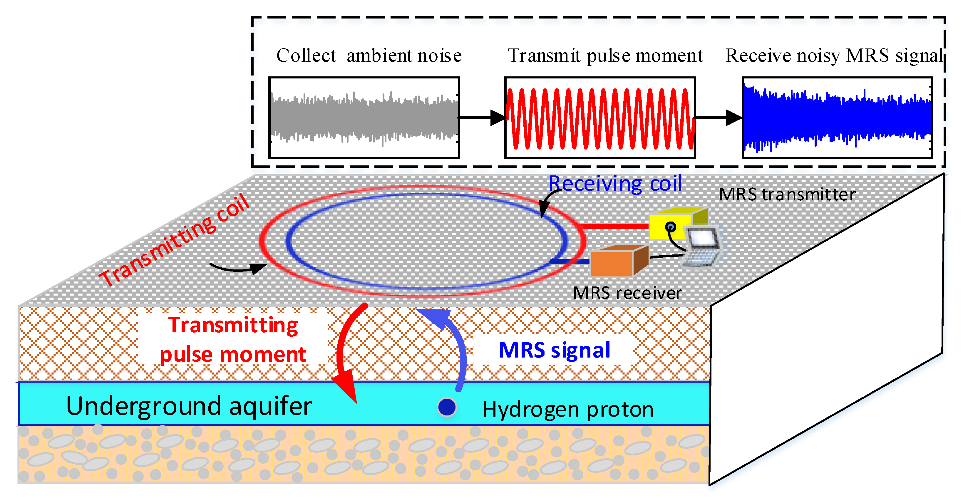
2.1. Noise and Signal in MRS Measurement

During the MRS measurement, the weak MRS signal is interfered by the surrounding electromagnetic noise, the noisy signal $s(t)$ received by the MRS instrument is always expressed as follows:

$$s(t)=nmr(t,q)+h(t)+p(t)+v(t)$$

(1)

where $t$ represents the recording time, $q$ is pulse moment, and $nmr(t,q)$, $h(t)$, $p(t)$, $v(t)$ denote MRS signal, harmonic noise, peak noise, random noise, respectively. Furthermore, the MRS signal can be expressed as:

$$nmr(t,q)=nm{r}_0(q)\cdot e^{(-t/T_2^{*}(q))}\cdot \cos (2\pi f_{Larmor}t+{\theta }_0(q))$$

(2)

where $nm{r}_0(q)$, $T_2^{*}(q)$, $f_{Larmor}$ and ${\theta }_0(q)$ are the signal parameters; they represent the initial amplitude, the relaxation time, the Larmor frequency and the initial phase of the MRS signal, respectively.

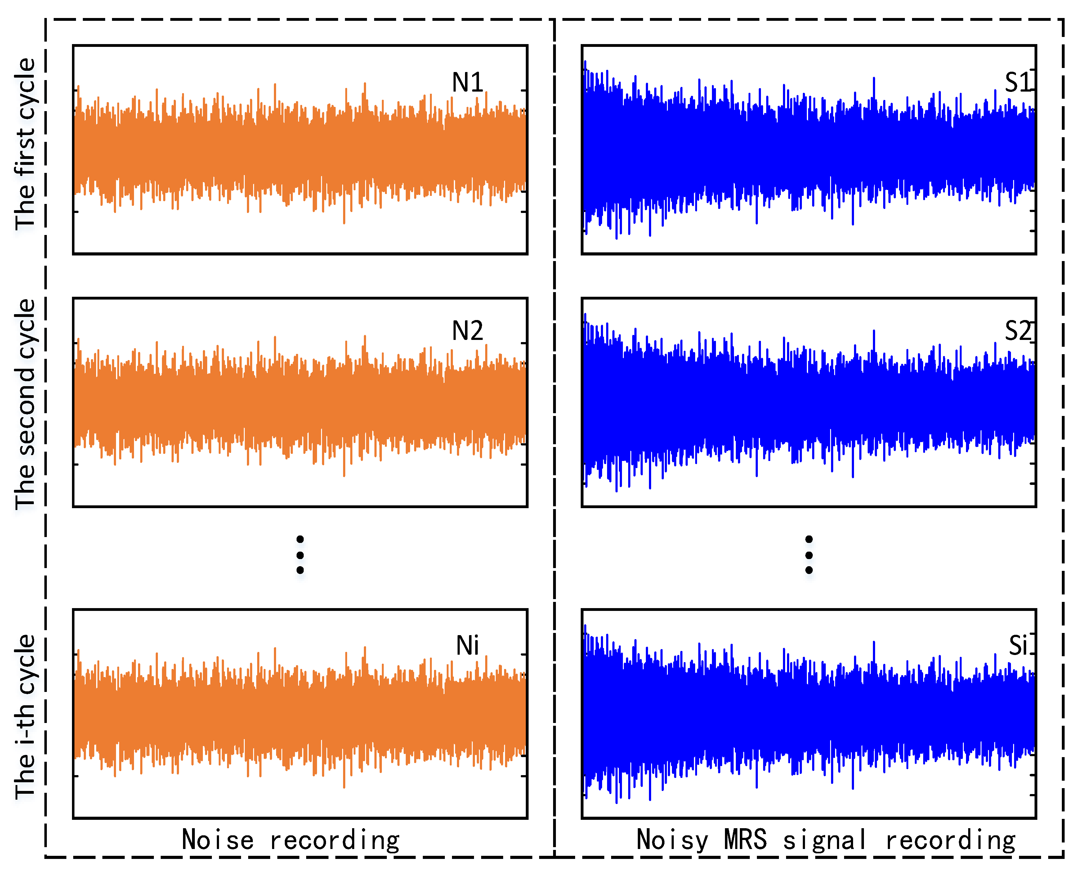
2.2. MRS Data Acquisition for DA-MFSS

When using the DA-MFSS method for noise suppression, we first collect multiple dataset, and then employ spectral subtraction to perform noise suppression on the collected data. Figure 1 shows the data acquisition procedure during MRS measurement.

From Figure 1, we can see that the ambient noise is first collected, then the noisy MRS signal is recorded. For example, the MRS receiver first collects the noise at the measurement site (N1 in Figure 1), then the MRS transmitter emits excitation current, and then the MRS receiver works again to receive the noisy MRS signal (S1 in Figure 1). By now, a cycle of the recording is completed. Then, the second cycle of the recording and the third cycle of the recording are repeated one by one. The left part of Figure 1 shows the pure noise. These noises will provide a noise spectrum during spectrum subtraction. The right part of Figure 1 illustrates the noisy MRS signals, which are used to provide the spectrum of noisy MRS signals.

After the acquisition of the pure noise and the noisy MRS signal, the multi-frame spectrum subtraction (MFSS) for noise suppression can be further performed. There are two methods to be selected for noise reduction. One is to process each data samples with MFSS separately. The other is using MFSS to process the stacked data. We know that the statistical average method is effective in SNR improvement. Besides, for the noise data collected in a different time, the spectrum of the stacked noise data may better represent the spectrum distribution of the ambient noise. Therefore, we prefer to utilize the stacked data using in MFSS.

According to the above analysis, when using the DA-MFSS method for noise suppression, the receiver of the MRS instrument first collects the pure noise at measurement site, then the transmitter transmits pulse current for 40 ms, and then the receiver collects the noisy MRS signal. The work procedure is shown in Figure 2.

2.3. Noise Suppression Procedure for DA-MFSS

After data acquisition, noise suppression by MFSS can be carried out, which mainly includes five processing stages. In order to illustrate the process procedure clearly, we conclude it and illustrate it in Figure 3.

The DA-MFSS mainly includes the following five steps.

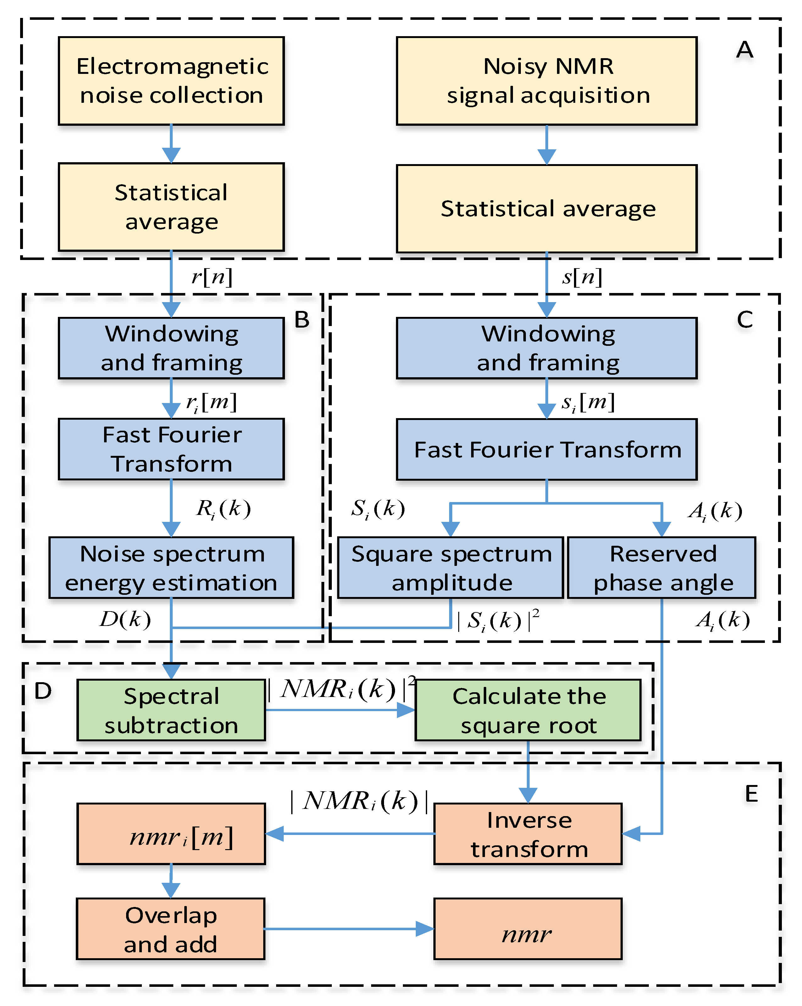
• Stage 1, the pure noise and the noisy MRS signals are calculated by statistical average, as shown in part A of Figure 3.
• Stage 2, the stacked noise is used to calculate the spectrum value at each frequency, as shown in part B of Figure 3.
• Stage 3, the stacked noisy MRS signal is applied to calculate the spectrum value at each frequency, as shown in part C of Figure 3.
• Stage 4, according to the MFSS theory, the above two spectral values are brought into the calculation of the energy value at different frequencies, as shown in part D of Figure 3.
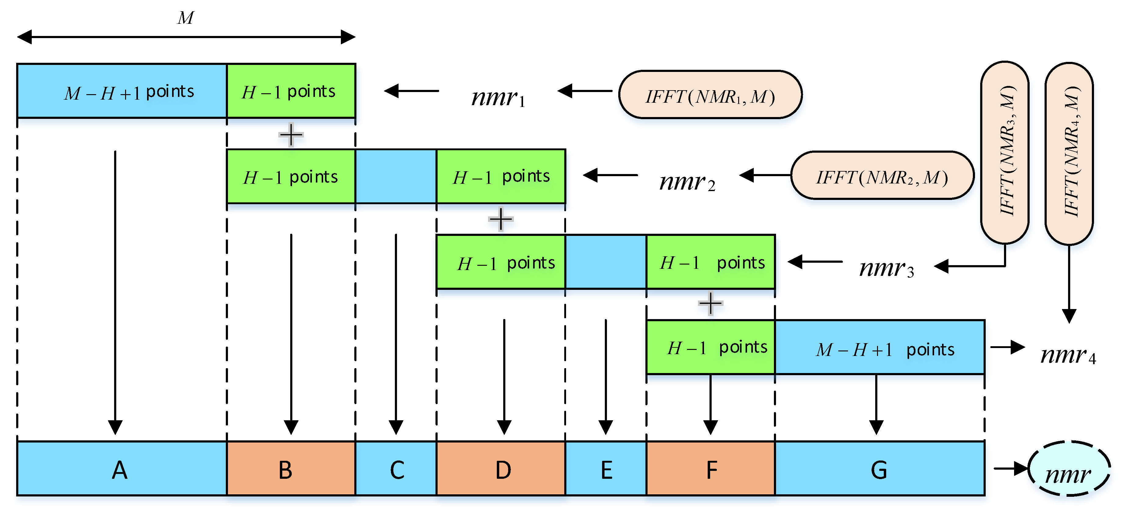
• Stage 5, based on inverse transformation formula and the overlap-add method, the MRS signal in the time domain after spectral subtraction is obtained, as shown in part E of Figure 3.

3. Noise Suppression Implementation of MFSS

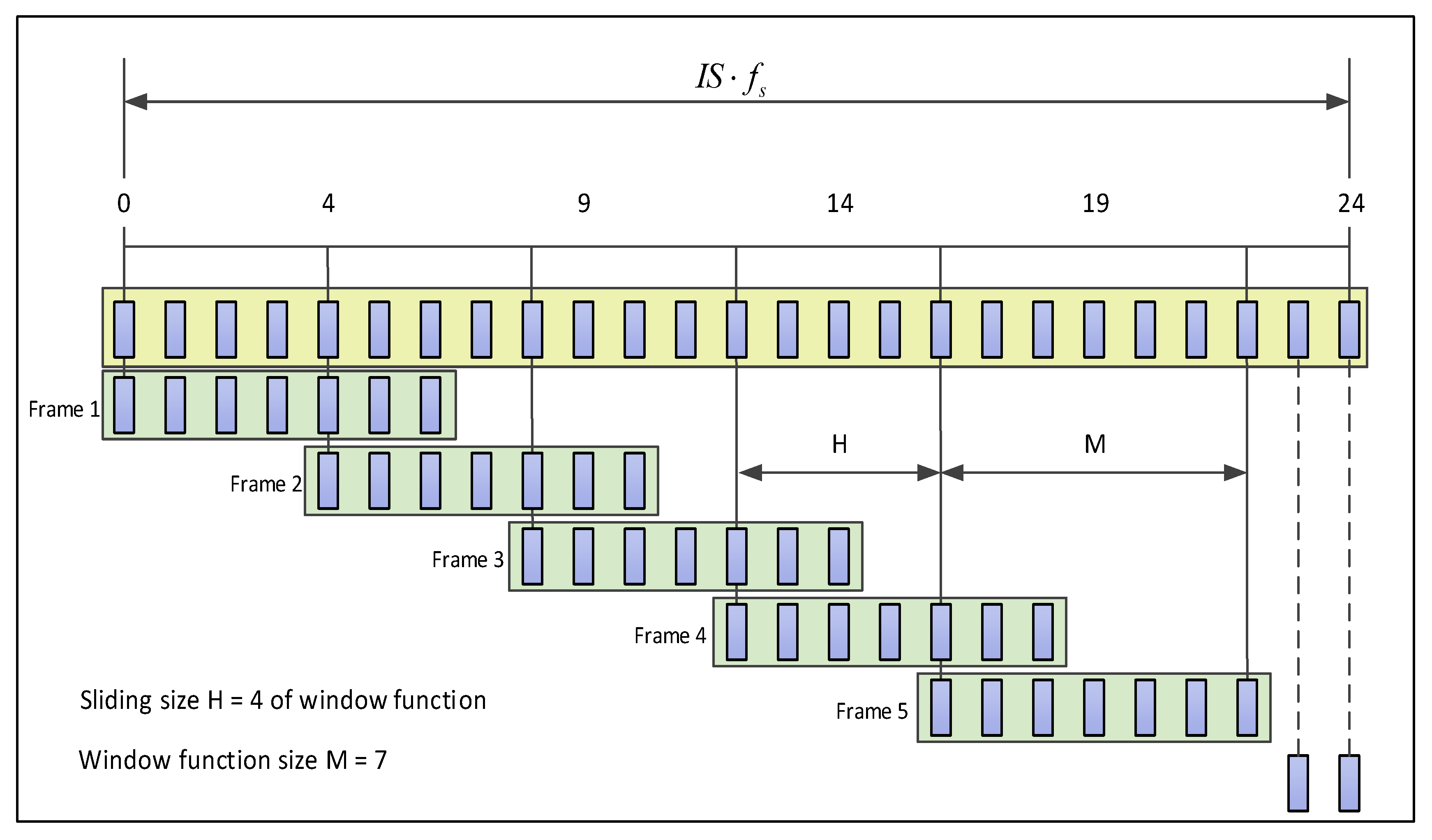
3.1. Discrete Fourier Transform of the Segmented Noisy MRS Signal

The stacked noisy MRS signal is expressed as discrete form $s[n]$. After adding window and framing, the i-th frame noisy signal is $s_i[m]$.

$$s_i[m]=s[m+iH]w[m]$$

(3)

where $i$ is the frame index, $w[\cdot ]$ represents window function, $H$ is the sliding size of the window function, $m$ denotes the time index within each frame, $m=1,\cdots ,M$, and $M$ is the frame length.

In order to show an excellent effect of noise suppression, here we list several common window functions for selection, as shown in

Table 1. Several common window functions.

Window Function	Time Domain Expression	Window Type
Rectangular window [25,26]	$w[m]=\{\begin{array}{l}1,\hspace{1em}\hspace{1em}m=0,1,\cdots ,M\\ 0,\hspace{1em}\hspace{1em}others\end{array}$	Power function type
Bartlett window [26,27,28]	$w[m]=\{\begin{array}{l}\frac{2m}{M},\hspace{1em}\hspace{1em}0\le m\le \frac{M}{2}\\ 2-\frac{2m}{M},\hspace{1em}\hspace{1em}\frac{M}{2}\le m\le M\end{array}$	Power function type
Hamming window [29,30]	$w[m]=\{\begin{array}{l}0.54-0.46\cos (2\pi \frac{m}{M}),\hspace{1em}\hspace{1em}0\le m\le M\\ 0,\hspace{1em}\hspace{1em}\hspace{1em}\hspace{1em}\hspace{1em}\hspace{1em}\hspace{1em}\hspace{1em}\hspace{1em} \hspace{1em}\hspace{1em}others\end{array}$	Trigonometric function type
Hanning window [31,32]	$w[m]=\{\begin{array}{l}0.5[1-\cos (2\pi \frac{m}{M})],\hspace{1em}\hspace{1em}0\le m\le M\\ 0,\hspace{1em}\hspace{1em}\hspace{1em}\hspace{1em}\hspace{1em}\hspace{1em}\hspace{1em}\hspace{1em}\hspace{1em} \hspace{1em}others\end{array}$	Trigonometric function type
Blackman window [33,34]	$w[m]=\{\begin{array}{l}0.42-0.5\cos (2\pi \frac{m}{M})+0.08\cos (4\pi \frac{m}{M}),\hspace{1em}0\le m\le \frac{M}{2}\\ 0,\hspace{1em}\hspace{1em}\hspace{1em}\hspace{1em}\hspace{1em}\hspace{1em}\hspace{1em}\hspace{1em}\hspace{1em}\hspace{1em}\hspace{1em}\hspace{1em}\hspace{1em}\hspace{1em} others\end{array}$	Trigonometric function type
Gaussian window [35,36]	$w[m]=\{\begin{array}{l}{e}^{-\frac{1}{2}{(\alpha \frac{2m}{M})}^2},\hspace{1em}\hspace{1em}-\frac{M}{2}\le m\le \frac{M}{2}\\ 0,\hspace{1em}\hspace{1em}\hspace{1em}\hspace{1em} \hspace{1em}\hspace{1em}others\end{array}$	Exponential function type

.

In order to compare the window shape in the time domain and the size of the main lobe and side lobe in the frequency domain more clearly, we compared the rectangular window, the Hamming window, the Blackman window and the Gaussian window, as shown in Figure 4.

From the comparison of the five windows in Figure 4, we can conclude that the main lobe of the rectangular window is narrowest, and its frequency resolution is the highest. The main lobe attenuation of the rectangular window is the smallest, but its side lobe attenuation is also small, which leads to serious energy leakage of the side lobe. The main lobe of the Hamming window is slightly wider than that of the rectangular window, so its frequency resolution is not as good as that of the rectangular window, but the side lobe attenuation of the Hamming window is larger than that of the rectangular window. The main lobe of the Hanning window is approximately equal to that of the Hamming window. The first side lobe of the Hanning window is bigger than the first side lobe of the Hamming window. The second side lobe attenuation of the Hanning window is close to that of the Hamming window. The third side lobe attenuation of the Hanning window is larger than that of the rectangular window, Hamming window and Gaussian window, but smaller than that of the Blackman window. The main lobe of the Blackman window is slightly wider than that of the Hamming window, that is, its frequency resolution is lower than that of the Hamming window. However, the side lobe attenuation of the Blackman window is the largest among the five kinds of windows, so its spectrum tailing is the smallest. In the figure, the main lobe of the Gaussian window is wider than that of the other four windows, and its frequency resolution is the lowest among the five windows. Nevertheless, the side lobe attenuation of the Gaussian window is larger than that of rectangular window and Hamming window, and smaller than that of the Blackman window and the Hanning window. Note that, when choosing a window function, we expect to choose a window function with a high-frequency resolution and small side lobe. However, due to the contradiction between the main lobe width and the attenuation of the side lobe, it is impossible to find the window function that can achieve both high-frequency resolution and very small side lobe. Therefore, when choosing the window function, according to the characteristics of actual data, we should choose an appropriate window function.

Based on the above discussion, we consider the tradeoff between the frequency resolution and the side lobe attenuation of window function, and choose the window function $w[m]$ as a Hamming window.

$$w[m]=0.54-0.46\cos (2\pi \frac{m}{M})\hspace{1em}\hspace{1em}\hspace{1em}0\le m\le M$$

(4)

where $m$ is the point index in the window function and $M$ is the window length.

Furthermore, in the frequency domain, the spectrum $S_i(k)$ of one frame $s_i[m]$ of noisy MRS signal $s[n]$ is obtained by discrete Fourier transform.

$$S_i(k)={\displaystyle \sum _{m=0}^{K-1}{s}_i[m]\exp (j\frac{2\pi mk}{K})}\hspace{1em}\hspace{1em}\hspace{1em}k=0,1,\cdots ,K-1$$

(5)

Here, $K$ is the total number of frequency points of one frame $s_i[m]$ in discrete Fourier transform, and $k$ is the frequency point index. From Equation (5), we can get the amplitude of the spectrum $S_i(k)$ at the k-th frequency point as follows:

$$|S_i(k)|=\sqrt{{[\mathrm{Im}(S_i(k))]}^2+{[\mathrm{Re}(S_i(k))]}^2}$$

(6)

Simultaneously, according to Equation (5), the phase $A_i(k)$ of the spectrum $S_i(k)$ at the frequency point $k$ in the i-th frame of noisy MRS data can be obtained.

$$A_i(k)=\arctan \left[\frac{\mathrm{Im}(S_i(k))}{\mathrm{Re}(S_i(k))}\right]$$

(7)

3.2. Energy Calculation of Each Frame Noise Data in the Frequency Domain

After the noise dataset is stacked, the representative noise $r[n]$ can be obtained, which can be expressed as follows:

$$r[n]=h[n]+p[n]+v[n]$$

(8)

where $h[n]$, $p[n]$ and $v[n]$ represent power-line harmonic noise, spike noise and random noise, respectively. Similarly, the typical noise $r[n]$ is windowed and framed.

$$r_i[m]=r[m+iH]w[m]$$

(9)

Furthermore, the spectrum $R_i(k)$ of the i-th frame noise $r_i[m]$ is obtained by discrete Fourier transform.

$$R_i(k)={\displaystyle \sum _{m=0}^{K-1}{r}_i(m)\exp (j\frac{2\pi mk}{K})}\hspace{1em}\hspace{1em}\hspace{1em}k=0,1,\cdots ,K-1$$

(10)

where $K$ is the total number of frequency points of one frame $r_i[m]$ in discrete Fourier transform, and $k$ denotes the frequency point index.

Assuming that the time length of the representative noise $r[n]$ obtained by statistical average is $IS$, then the corresponding frame number is $NIS$:

$$NIS=\lfloor \frac{IS\cdot f_s-M}{H}\rfloor +1$$

(11)

where the operator $\lfloor ·\rfloor$ describes solving the maximum integer corresponding to a real number.

In order to explain the calculation principle of the number of frames when the representative noise data $r[n]$ is divided into frames, we give Figure 5 for description. In this figure, we take the noise data with 25 sampling points as an example, in which the small rectangular block represents a sampling point, such as sampling point 0, sampling point 4 and sampling point 9, etc. If the window length $M$ = 7 and the sliding step $H$ = 4, then the noise data can be divided into five frames. On the other hand, we calculate $NIS=\lfloor \frac{24-7}{4}\rfloor +1=5$ by Equation (11). According to Figure 5, we conclude that the actual total number of frames is equal to the calculated total number of frames. Therefore, when calculating the total number of frames, the total number of frames of the whole data can be calculated quickly through Equation (11).

According to Equations (10) and (11), the average energy value $D(k)$ of the spectrum at the frequency point k of the representative noise $r[n]$ is as follows:

$$D(k)=\frac{1}{NIS}{\displaystyle \sum _{i=1}^{NIS}|R_i(k){|}^2}$$

(12)

3.3. MRS Signal Estimation by MFSS

After obtaining the spectrum $S_i(k)$ of the noisy MRS signal $s[n]$ and the average energy $D(k)$ of the representative noise $r[n]$, we can use MFSS to estimate the energy $E{N}_i(k)$ of the i-th frame data of MRS signal at the frequency point k.

$$E{N}_i(k)=|{\widehat{NMR}}_i(k){|}^2=\{\begin{array}{l}|S_i(k){|}^2-\alpha \cdot D(k)\hspace{1em}\hspace{1em}|S_i(k){|}^2\ge \alpha \cdot D(k)\\ \beta \cdot D(k)\hspace{1em}\hspace{1em}\hspace{0.17em}\hspace{1em}\hspace{1em}\hspace{1em}\hspace{0.17em}\hspace{0.17em}\hspace{0.17em}|S_i(k){|}^2<\alpha \cdot D(k)\end{array}$$

(13)

where $\alpha$ is the judgment factor of spectral subtraction, $\beta$ is the gain compensation factor.

According to Equation (13), the estimated amplitude $|{\widehat{NMR}}_i(k)|$ of MRS signal is obtained, and then a new spectrum can be constructed by combining the phase angle $A_i(k)$ estimated by Equation (7), for example, the spectrum of the i-th frame at frequency point $k$ is as follows.

$${\widehat{NMR}}_i(k)=\sqrt{EN(k)}\exp [jA(k)]$$

(14)

Furthermore, in the light of Equation (14), the spectral values of each frequency point of the i-th frame can be obtained, so that the estimated spectrum ${\widehat{NMR}}_i$ of the i-th frame can be acquired.

Then, through the fast Fourier inverse transform, we can get the i-th frame estimated signal ${\widehat{nmr}}_i$ with the length M in the time domain

$${\widehat{nmr}}_i=IFFT({\widehat{NMR}}_i,M)$$

(15)

where $IFFT$ represents fast Fourier inverse transform, and ${\widehat{nmr}}_i$ denotes the i-th frame MRS signal estimation in the time domain according to the estimated spectrum ${\widehat{NMR}}_i$ and the time domain length M.

According to Equation (15), the estimated MRS signals are segmented, and they cannot be directly and simply spliced into a complete MRS signal. In order to obtain a complete MRS signal, we apply the overlap-add method to construct the complete MRS signal. To illustrate the overlap-add method to estimate the complete MRS signal, we draw Figure 6 to describe the signal construction. In the figure, according to Equations (13) and (14), the estimated spectrum ${\widehat{NMR}}_i$ of the i-th frame can be obtained, for example, the estimated spectrum ${\widehat{NMR}}_1$, ${\widehat{NMR}}_2$, ${\widehat{NMR}}_3$, ${\widehat{NMR}}_4$, etc. Then, the i-th frame estimated signal ${\widehat{nmr}}_i$ with the length M in the time domain can be further obtained through the fast Fourier inverse transform, such as the first frame estimated signal ${\widehat{nmr}}_1$, the second frame estimated signal ${\widehat{nmr}}_2$, the third frame estimated signal ${\widehat{nmr}}_3$, the fourth frame estimated signal ${\widehat{nmr}}_4$, etc. Furthermore, according to the frame length M and the sliding size H of the window function, the estimated signal ${\widehat{nmr}}_1$ with the length M is divided into the front part with the length $M-H+1$ and the latter part with the length $H-1$. The estimated signal ${\widehat{nmr}}_2$ with the length M is divided into three parts: the left part with the length H-1, the middle part with the length $M-2H+2$, the right part with the length $H-1$. Similarly, ${\widehat{nmr}}_3$ and ${\widehat{nmr}}_4$ are divided into parts as shown in Figure 6. Finally, the front part with the length $M-H+1$ of the estimated signal ${\widehat{nmr}}_1$ is directly Part A of the complete MRS signal $\widehat{nmr}$, and then the latter part with the length $H-1$ of the estimated signal ${\widehat{nmr}}_1$ and the left part with the length $H-1$ of the estimated signal ${\widehat{nmr}}_2$ are correspondingly added to form Part B of the complete MRS signal $\widehat{nmr}$. In the same way, we can get Part C, Part D, Part E, Part F and Part G of the complete MRS signal.

From Figure 6, we can conclude that according to the calculated ${\widehat{nmr}}_1$, ${\widehat{nmr}}_2$, ${\widehat{nmr}}_3$, ⋯ ${\widehat{nmr}}_i$ by Equation (15), we can construct the estimated complete MRS signal $\widehat{nmr}$ through the overlap-add method.

4. Noise Suppression Experiments of DA-MFSS

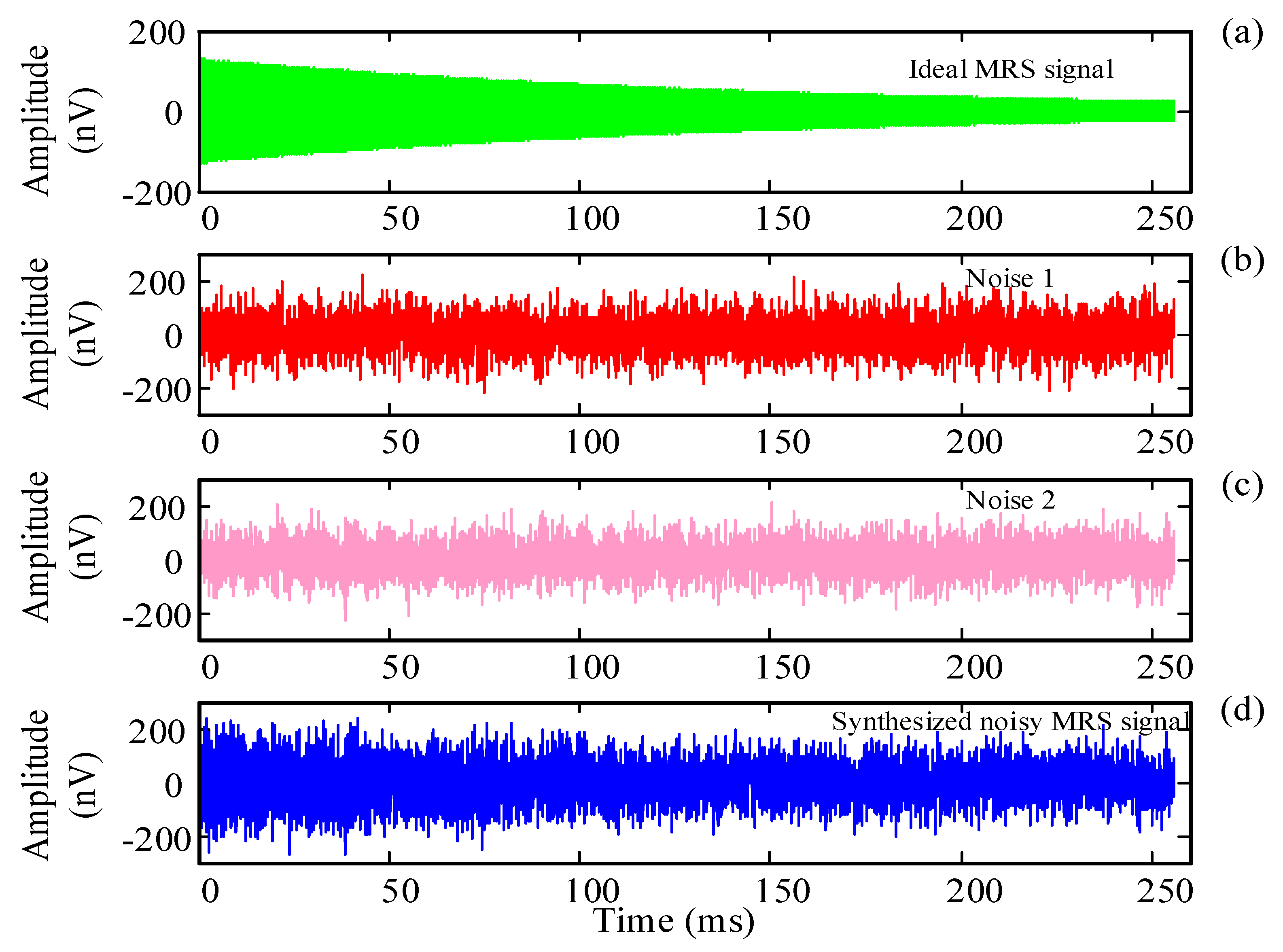
4.1. Simulation Experiment

In order to verify the noise suppression effect of DA-MFSS, we utilize the synthetic noisy MRS data to conduct a simulation experiment.

The initial amplitude $nm{r}_0(q)$, the apparent relaxation time $T_2^{*}(q)$, the Larmor frequency $f_{Larmor}$ and the initial phase angle ${\phi }_0(q)$ of the ideal MRS signal are set as shown in

Table 2. Parameters setting of the ideal MRS signal.

Parameter Name	$\mathit{n}\mathit{m}{\mathit{r}}_0(\mathit{q})\left[\mathbf{nV}\right]$	${\mathit{T}}_2^{*}(\mathit{q})\left[\mathbf{ms}\right]$	${\mathit{f}}_{\mathit{L}\mathit{a}\mathit{r}\mathit{m}\mathit{o}\mathit{r}}\left[\mathbf{Hz}\right]$	${\mathit{\phi }}_0(\mathit{q})\left[\mathbf{rad}\right]$
Value	130	150	2335	0

. In the simulated noisy MRS signal, the ideal MRS signal and the noise is included. The parameters of noise added in the synthesis is shown in

Table 3. The parameters setting of the noise.

Parameter name	Mean Value [nV]	Standard Deviation [nV]	Noise Type
Value	−0.19	61.45	Gaussian noise

.

In the simulation experiment, we set the recording time length to 256 ms and the sampling frequency $f_s$ = 25 kHz. In order to facilitate the comparison with the synthesized noisy MRS signal after noise suppression, this section shows the synthesis process of the noisy MRS signal in Figure 7. Figure 7a shows the ideal MRS signal. The ideal signal parameters are shown in Table 2. Figure 7b shows the Gaussian noise 1, and its parameters are shown in Table 3. Figure 7d shows the noisy MRS signal corrupted with noise 1, in which the SNR is −1.61 dB. To make the noise closer to the actual noise, Figure 7c shows Gaussian noise 2 with the mean value of −0.19 nV and the standard deviation of 61.45 nV, but it is different from noise 1 shown in Figure 7b.

In the noise suppression process of DA-MFSS, we set the window function as Hamming window, the window length as M = 1200 (1200/$f_s$ = 48 ms), and the frame shift as H = 600 (600/$f_s$ = 24 ms). We choose the judgment factor $\alpha$ = 9.8 and the gain compensation factor $\beta$ = 0.001. Simultaneously, the Gaussian noise 2 is selected as the noise of spectral subtraction. According to the noise suppression steps of MFSS in Figure 3, after noise elimination the SNR of MRS data reaches 15.27 dB. Furthermore, in order to compare the waveforms before and after MRS data denoising, Figure 8 is drawn to illustrate the noise suppression effect of MFSS. From the figure, we can conclude that the de-noised MRS signal is close to the ideal MRS signal, and the noise is eliminated. Moreover, the SNR is improved by 16.89 dB.

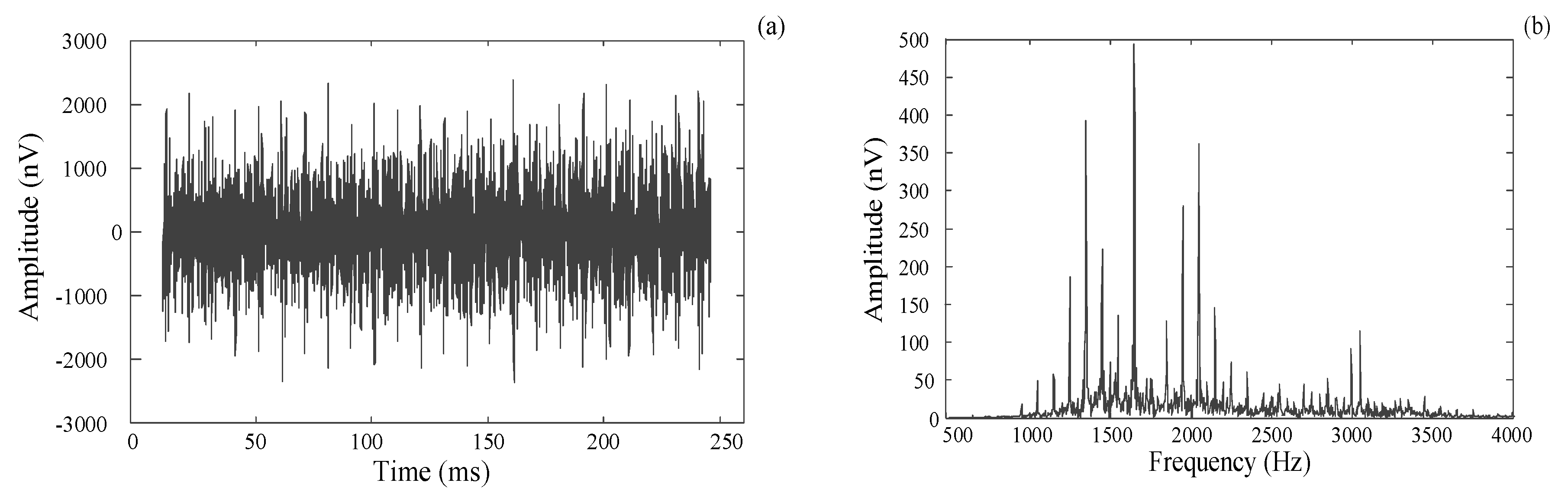
4.2. Field Data Processing

In order to verify the performance of DA-MFSS, we utilized the JLMRS instrument [13] to carry out a field experiment in Shaoguo Town, Changchun City, Jilin Province, China. In the field experiment, the adopted data acquisition method is as described in Section 2, that is, in each acquisition cycle, the pure noise data are collected first, then the excitation pulse moment is transmitted, and then the noisy magnetic resonance signal is collected. In the field experiment, the adopted data acquisition method is as described in the second section, that is to collect the noise data first, then transmit the excitation pulse moment, and then collect the noisy MRS signal. The transmitting coil and receiving coil are both single turn square coil with 100 m × 100 m, the single transmitting current duration is 40 ms, and the single recording duration is 256 ms. After laying the coil and setting up the MRS instrument, we performed 32 stacks, and then average the recorded data to calculate the pure noise $r[n]$ and the noisy MRS signal $s[n]$. According to the steps in Figure 3, through the statistical average for the data, the stacked noise is obtained, as is shown in Figure 9. Figure 9a shows the pure noise $r[n]$ and Figure 9b shows the amplitude spectrum of the representative noise $r[n]$ in the frequency domain. From the figure, it can be concluded that the electromagnetic noise from the measurement area is large and complex.

Similarly, the collected noisy MRS data is processed by stacking. Figure 10a shows the noisy MRS signal $s[n]$ and Figure 10b shows the amplitude spectrum of the noisy MRS signal $s[n]$. According to the figure, we can conclude that a large amount of harmonic noise and random noise completely submerge the MRS signal, and the trend of the MRS signal cannot be found in the time domain.

Next, we analyze the selection of parameters in two cases to obtain a better noise reduction effect of spectral subtraction.

4.2.1. Select Short Frame Length and Small Frame Sliding Distance

In the noise reduction through MFSS, we still set the window function as a Hamming window, the short frame length as M = 1200 and the small frame shift as H = 600. Taking the representative noise $r[n]$ as the noise used for spectral subtraction, we select the judgment factor $\alpha$ = 4.28 and the gain compensation factor $\beta$ = 0.001. According to the steps of DA-MFSS in Figure 3, the standard deviation of the noisy MRS signal (shown in Figure 10) is reduced to 386.40 nV from 741.37 prior to multi-frame spectral subtraction.

The comparison before and after noise reduction is shown in Figure 11a. It can be seen from the figure that the noise is suppressed though MFSS. From Figure 11b, we can conclude that, through spectral subtraction, in addition to the random noise being suppressed, the harmonic noise at multiple power frequencies is also suppressed. Moreover, the noise around the Larmor frequency is also suppressed. Based on noise suppression by DA-MFSS, we utilize a band-pass filter with band-pass range of 2320 Hz to 2350 Hz to extract the envelope of MRS signal with the initial amplitude of 413.37 nV and the apparent relaxation time of 124.90 ms, as shown in Figure 11a.

4.2.2. Select Long Frame Length and Large Frame Sliding Distance

In the case of long frame length and large sliding distance, we still set the window function as the Hamming window, but the frame length is 2600 and the frame shift is 1300. Taking the pure noise $r[n]$ in Figure 9 as the noise used for spectral subtraction, we select the judgment factor $\alpha$ = 9.29 and the gain compensation factor $\beta$ = 0.0001. In the light of the steps in Figure 3, the standard deviation of the noisy MRS signal (shown in Figure 10) is reduced to 157.57 nV from 741.37 nV prior to MFSS.

The noise reduction result is shown in Figure 12 under the condition of long frame length and large frame sliding distance. It can be seen from the figure that the noise is greatly suppressed though MFSS. From Figure 12b, we can conclude that by the spectral subtraction, in addition to the random noise being suppressed, the harmonic noise at multiple power frequencies is also effectively suppressed. Moreover, the noise around the Larmor frequency is also suppressed. Based on noise suppression by DA-MFSS, we utilize a band-pass filter with a band-pass range of 2320 to 2350 Hz to extract the envelope of MRS signal with the initial amplitude of 408.31 nV and the apparent relaxation time of 141.97 ms, as shown in Figure 12a.

Compared with Figure 11 and Figure 12, it is concluded that, in the case of long window length, large frame shift and large the judgment factor, the better noise suppression effect can be obtained. For the convenience of observing the residual noise, we plot the amplitude spectrum after DA-MFSS in Figure 13.

According to Figure 13, by DA-MFSS, the random noise is effectively suppressed. Most of the power frequency harmonic noise is also suppressed; however, there are still some power frequency harmonic noise residues (such as frequency points p’3, p’7, p’13 and p’15). Specifically, the residual power frequency harmonic noise at 1751, 2402, 3155 and 3250 Hz has not been completely eliminated, but the residual harmonic noise is much smaller than the power frequency harmonic in Figure 12.

5. Discussion

According to the previous parts, we can conclude that the DA-MFSS can not only suppress the random noise, but also eliminate the interference of harmonic noise. This method provides a new idea to deal with the noise embedded in the MRS data, which can process multiple types of noise at one time in the noise processing process. It can be seen from the results of simulation experiment and field experiment that the proposed method based on DA-MFSS has an excellent de-noising effect on MRS data containing complex noise.

The data used in DA-MFSS are the stacking data. Since the noise used in stacking comes from different time periods, the spectral value obtained from the noise data by stacking at each frequency can better reflect and represent the noise spectrum distribution around the measurement site. Therefore, the statistical averaging is not only conducive to the elimination of random noise, but also conducive to multi-frame spectral subtraction.

In DA-MFSS, the difference of denoising effect is related to the frame length, the judgment factor α and the gain compensation factor β. When setting the long window length, the large judgment factor and the small gain compensation factor (for example, the window length M = 2600, the frame shift H = 1300, the judgment factor α = 9.29, the gain compensation factor β = 0.0001), the good noise elimination effect can be obtained, as shown in Figure 12. However, when setting short window length and small judgment factor (for example, the window length M = 1200, the judgment factor α = 4.28), the noise suppression effect is somewhat reduced, as shown in Figure 11. Therefore, when using DA-MFSS to suppress noise, it is necessary to reasonably choose a relatively large window length, large judgment factor and small gain compensation factor.

6. Conclusions

In this paper, focusing on the noise interference of noisy MRS signals, the noise and noisy data acquisition and the theory of spectral subtraction are studied, respectively. The noise-suppression method based on data acquisition and multi-frame spectral subtraction (DA-MFSS) is proposed to process the noisy MRS data.

The method first collects pure noise through the receiving coil in the measurement area, and then collects the noisy MRS signal after transmitting pulse moments. The pure noise and the noisy MRS signal acquisition are repeated for several times, and then the pure noise and the noisy signal are statistically averaged to obtain the representative data prior to MFSS. Then, the MFSS is used to suppress noise of the segmented noisy MRS data. Furthermore, the overlap-add method is utilized to synthesize the segmented estimated signals into the complete MRS signal. Finally, through the numerical simulation and noise suppression verification of on-site noisy MRS data, the SNR of the MRS data can be improved by 16.89 dB, and the method proposed in this paper can well suppress random noise and harmonic noise. This method has the advantage of suppressing multiple types of noise at the same time, making up for the shortcomings of the traditional noise-suppression method in MRS data processing.

References

1. Hertrich, M.; Braun, M.; Gunther, T.; Green, A.G.; Yaramanci, U. Surface nuclear magnetic resonance tomography. IEEE Trans. Geosci. Remote Sens. 2007, 45, 3752–3759. [Google Scholar] [CrossRef]
2. Legchenko, A. Magnetic Resonance Imaging for Groundwater; ISTE Ltd.: London, UK, 2013. [Google Scholar]
3. Legchenko, A.; Valla, P. A review of the basic principles for proton magnetic resonance sounding measurements. J. Appl. Geophys. 2002, 50, 3–19. [Google Scholar] [CrossRef]
4. Du, G.; Lin, J.; Zhang, J.; Yi, X.; Jiang, C. Study on shortening the dead time of surface nuclear magnetic resonance instrument using bipolar phase pulses. IEEE Trans. Instrum. Meas. 2020, 69, 1268–1274. [Google Scholar] [CrossRef]
5. Legchenko, A.; Valla, P. Removal of power-line harmonics from proton magnetic resonance measurements. J. Appl. Geophys. 2003, 53, 10–120. [Google Scholar] [CrossRef]
6. Lin, T.; Yang, Y.J.; Yang, Y.; Wan, L.; Teng, F. Exploiting adiabatic pulses with prepolarization in detection of underground nuclear magnetic resonant signals. IEEE Trans. Geosci. Remote Sens. 2019, 57, 4558–4567. [Google Scholar] [CrossRef]
7. Lin, T.; Zhang, Y.; Yi, X.; Fan, T.; Wan, L. Time–frequency peak filtering for random noise attenuation of magnetic resonance sounding signal. Geophys. J. Int. 2018, 213, 727–738. [Google Scholar] [CrossRef]
8. Walsh, D.O. Multi-channel surface NMR instrumentation and software for 1D/2D groundwater investigations. J. Appl. Geophys. 2008, 66, 140–150. [Google Scholar] [CrossRef]
9. Grunewald, E.; Grombacher, D.; Walsh, D. Adiabatic pulses enhance surface nuclear magnetic resonance measurement and survey speed for groundwater investigations. Geophysics 2016, 81, WB85–WB96. [Google Scholar] [CrossRef]
10. Müller-Petke, M.; Braun, M.; Hertrich, M.; Costabel, S.; Walbrecker, J. MRSmatlab—a software tool for processing, modeling, and inversion of magnetic resonance sounding data. Geophysics 2016, 81, WB9–WB21. [Google Scholar] [CrossRef]
11. Falzone, S.; Keating, K. Algorithms for removing surface water signals from surface nuclear magnetic resonance infiltration surveys. Geophysics 2016, 81, WB97–WB107. [Google Scholar] [CrossRef]
12. Müller-Petke, M.; Yaramanci, U. QT inversion—Comprehensive use of the complete surface NMR data set. Geophysics 2010, 75, WA199–WA209. [Google Scholar] [CrossRef]
13. Jiang, C.; Lin, J.; Duan, Q.; Sun, S.; Tian, B. Statistical stacking and adaptive notch filter to remove high-level electromagnetic noise from MRS measurements. Near Surf. Geophys. 2011, 9, 459–468. [Google Scholar] [CrossRef]
14. Dalgaard, E.; Auken, E.; Larsen, J.J. Adaptive noise cancelling of multichannel magnetic resonance sounding signals. Geophys. J. Int. 2012, 191, 88–100. [Google Scholar] [CrossRef]
15. Larsen, J.; Dalgaard, E.; Auken, E. Noise cancelling of MRS signals combining model-based removal of powerline harmonics and multichannel Wiener filtering. Geophys. J. Int. 2014, 196, 828–836. [Google Scholar] [CrossRef] [Green Version]
16. Larsen, J.J. Model-based subtraction of spikes from surface nuclear magnetic resonance data. Geophysics 2016, 81, WB1–WB8. [Google Scholar] [CrossRef] [Green Version]
17. Costabel, S.; Müller-Petke, M. Despiking of magnetic resonance signals in time and wavelet domains. Near Surf. Geophys. 2014, 12, 185–197. [Google Scholar] [CrossRef]
18. Lin, T.; Zhang, Y.; Müller-Petke, M. Random noise suppression of magnetic resonance sounding oscillating signal by combining empirical mode decomposition and time-frequency peak filtering. IEEE Access 2019, 7, 79917–79926. [Google Scholar] [CrossRef]
19. Yao, X.; Zhang, J.; Yu, Z.; Zhao, F.; Sun, Y. Random noise suppression of magnetic resonance sounding data with intensive sampling sparse reconstruction and kernel regression estimation. Remote Sens. 2019, 11, 1829. [Google Scholar] [CrossRef] [Green Version]
20. Boll, S. Suppression of acoustic noise in speech using spectral subtraction. IEEE Trans. Acoust. Speech Signal Process. 1979, 27, 113–120. [Google Scholar] [CrossRef] [Green Version]
21. Gruden, S.; Zajc, B. Using spectral subtraction for suppression of noise in speech signals with analog integrated circuits. Analog Integr. Circuits Process. 1999, 18, 195–207. [Google Scholar] [CrossRef]
22. Yamashita, K.; Shimamura, T. Non-stationary noise estimation using low-frequency regions for spectral subtraction. IEEE Signal Process. Lett. 2005, 12, 465–468. [Google Scholar] [CrossRef]
23. Chen, Z.; Wang, R.; Yin, F. Speech dereverberation method based on spectral subtraction and spectral line enhancement. Appl. Acoust. 2016, 112, 201–210. [Google Scholar] [CrossRef]
24. Fatemeh, A.; Antoine, T.; Marc, T. Tool condition monitoring using spectral subtraction and convolutional neural networks in milling process. Int. J. Adv. Manuf. Technol. 2018, 98, 3217–3227. [Google Scholar]
25. Mohindru, P.; Khanna, R.; Bhatia, S.S. New tuning model for rectangular windowed FIR filter using fractional Fourier transform. Signal Image Video Process. 2015, 9, 761–767. [Google Scholar] [CrossRef]
26. Ha, Y.H.; Pearce, J.A. A new window and comparison to standard windows. IEEE Trans. Acoust. Speech Signal Process. 1989, 37, 298–301. [Google Scholar] [CrossRef]
27. Agarwal, P.; Singh, S.P.; Pandey, V.K. Spectrum shaping analysis using tunable parameter of fractional based on Bartlett window. In Proceeding of the 3rd IEEE International Advance Computing Conference, Ghaziabad, India, 22–23 February 2013; pp. 1625–1630. [Google Scholar]
28. Wang, G.; Wang, X.; Zhao, C. An Iterative Hybrid Harmonics Detection Method Based on Discrete Wavelet Transform and Bartlett–Hann Window. Appl. Sci. 2020, 10, 3922. [Google Scholar] [CrossRef]
29. Bojkovic, Z.S.; Bakmaz, B.M.; Bakmaz, M.R. Hamming Window to the Digital World. Proc. IEEE 2017, 105, 1185–1190. [Google Scholar] [CrossRef]
30. Basit, A.; Qureshi, I.M.; Khan, W.; ur Rehman, S.; Khan, M.M. Beam Pattern Synthesis for an FDA Radar with Hamming Window-Based Nonuniform Frequency Offset. IEEE Antennas Wirel. Propag. Lett. 2017, 16, 2283–2286. [Google Scholar] [CrossRef]
31. Chen, J.; Wang, W.; Wang, S.H.; Yang, S.M. An approach for electrical harmonic FFT analysis based on Hanning self-multiply window. Power Syst. Prot. Control. 2016, 19, 114–121. [Google Scholar]
32. Chen, K.F.; Mei, S.L. Composite Interpolated Fast Fourier Transform with the Hanning Window. IEEE Trans. Instrum. Meas. 2010, 59, 1571–1579. [Google Scholar] [CrossRef]
33. Roh, H.J.; Kim, N.K.; Ryu, S.; Park, S.; Lee, S.H.; Huh, S.R.; Kim, G.H. Determination of electron energy probability function in low-temperature plasmas from current-Voltage characteristics of two Langmuir probes filtered by Savitzky-Golay and Blackman window methods. Curr. Appl. Phys. 2015, 15, 1173–1183. [Google Scholar] [CrossRef]
34. Soni, R.K.; Jain, A.; Saxena, R. An improved and simplified design of pseudo-transmultiplexer using Blackman window family. Digit. Signal Prog. 2010, 20, 743–749. [Google Scholar] [CrossRef]
35. Wang, Y.; Cao, R.; Huang, X. ISAR imaging of maneuvering target based on the estimation of time varying amplitude with Gaussian window. IEEE Sens. J. 2019, 19, 11180–11191. [Google Scholar] [CrossRef]
36. Goel, N.; Singh, J. Analysis of Kaiser and Gaussian Window Functions in the Fractional Fourier Transform Domain and Its Application. Iran. J. Sci. Technol. Trans. Electr. Eng. 2019, 43, 181–188. [Google Scholar] [CrossRef]
Figure 1. Schematic diagram of the magnetic resonance sounding (MRS) data acquisition procedure for data acquisition and multi-frame spectral subtraction (DA-MFSS).
Electronics 09 01254 g001
Figure 2. Measurement diagram for the MRS data acquisition.
Electronics 09 01254 g002
Figure 3. Algorithm flowchart of DA-MFSS. In part A, the data collection and statistical average; In part B, calculating the spectrum of the stacked noise; In part C, calculating the spectrum of the stacked noisy MRS signal; In part D, multi-frame spectral subtraction of the above two spectrum; In part E, calculating the MRS signal in the time domain through the inverse transformation and the overlap-add method.
Electronics 09 01254 g003
Figure 4. Comparison of several common window functions in the time domain and frequency domain (window length M = 65).
Electronics 09 01254 g004
Figure 5. Calculation of the total frames of noise data.
Electronics 09 01254 g005
Figure 6. Estimated MRS signal construction via the overlap-add method after multi-frame spectral subtraction and fast Fourier inverse transform.
Electronics 09 01254 g006
Figure 7. Simulation of noisy MRS signal. (a) The ideal MRS signal without noise; (b) the simulated noise 1; (c) the simulated noise 2 for MFSS; (d) the simulated noisy MRS signal with the noise 1.
Electronics 09 01254 g007
Figure 8. Noise suppression result using DA-MFSS.
Electronics 09 01254 g008
Figure 9. Pure noise r [ n ] obtained by stacking. (a) The pure noise in the time domain; (b) the corresponding amplitude spectrum.
Electronics 09 01254 g009
Figure 10. Noisy MRS signal s [ n ] obtained by stacking. (a) The noisy MRS signal in the time domain; (b) the corresponding amplitude spectrum in the frequency domain.
Electronics 09 01254 g010
Figure 11. Noise reduction result of field MRS data by MFSS under the condition of short window length and small frame shift. (a) The waveform comparison and the extracted envelope; (b) the spectral amplitude comparison.
Electronics 09 01254 g011
Figure 12. Noise reduction of field MRS data by MFSS under the condition of long frame length and large sliding distance. (a) The waveform comparison and the extracted envelope; (b) the spectral amplitude comparison.
Electronics 09 01254 g012aElectronics 09 01254 g012b
Figure 13. Comparison of residual noise and MRS signal by DA-MFSS.
Electronics 09 01254 g013