1. Introduction
Positioning has been a topic of interest for both industry and the research community for many years. However, the massive spread of sensors and mobile wireless communication devices as a result of the Internet of the Things (IoT) paradigm has boosted the interest in location. A great number of current and future applications and services can greatly benefit from the knowledge of where their users (i.e., devices) are, such as in the fields of elderly people healthcare, personnel and asset tracking, emergency services, disabled people guiding assistance, traffic control, factory automation, etc. [
1].
For the last few years, Global Navigation Satellite System (GNSS) techniques have mastered outdoor positioning, especially those based on Global Positioning System (GPS). However, these techniques are known to drastically lose reliability indoors, even providing no position at all under severe indoor conditions [
2]. Furthermore, they usually require a noticeable computational effort to fix positions, which greatly reduces the battery lifetime of unplugged devices and relegates GNSS techniques to powerful enough mobile devices only (e.g., mobile phones used outdoors). Despite the limitations, there is no global location solution yet that applies to both indoor and outdoor environments with the same extent as GNSS in outdoor environments.
The scenario of heterogeneous systems, multiple environments, device hyperconnectivity, and contextualized services, drawn by the IoT paradigm, has paved the way to several location technique proposals. These techniques can be split into: (1) those requiring specific location network infrastructure, and (2) those relying on regular communication networks already deployed. The former group includes techniques that use custom devices to gather the location information required to compute the device’s position. Some of these techniques, such as those based on Ultra-Wide Band (UWB) [
3], focus on maximizing the accuracy. Others, such as those based on Radio Frequency Identification (RFID) [
3], which is often used for stock monitoring, aim at minimizing the deployment cost while maintaining fair performance. However, all of these techniques require their own mobile devices to be attached to any traceable item, which is a major drawback for mass-market global positioning solutions. Another related approach, based on computer vision, is covered throughout in [
4]. Computer vision has the benefit of working consistently, whatever the environment, i.e., indoors or outdoors. However, it requires either video/image capture devices to be deployed in the network or convenient sensors at the user equipment. Furthermore, it often demands complex positioning algorithms that frequently come with high computational effort requirements. Accordingly, the use of these techniques is limited in the IoT context.
The second group includes all the techniques that make use of an already deployed communication network to gather the location information, such as Public Land Mobile Networks (PLMN), Bluetooth Low Energy (BLE), and IEEE 802.11. As the aim of this paper is to propose a globally available solution for indoor scenarios, the authors have focused on these technologies that are known to be readily available in commercial off-the-shelf (COTS) devices. While BLE-based techniques provide accurate positions, the availability of the system for positioning purposes cannot be ensured due to the ad hoc nature of the BLE network. In contrast, PLMN and IEEE 802.11 networks are considered to be available everywhere, ensuring the global availability a GNSS-like solution should provide. Despite providing positioning capabilities since their third generation (i.e., UMTS, CDMA-2000, etc.), PLMNs are rarely used due to the poor performance they provide indoors [
1], where signals are blocked (e.g., when crossing walls) and reported positions are consequently inaccurate.
For all the above, the main focus of our proposal is on IEEE 802.11 (i.e., WiFi) networks, which are densely deployed indoors and outdoors in the case of urban and dense urban scenarios, such as those drawn in smart cities. The global availability and high density of WiFi networks make this technology ideal for positioning. A few years ago, IEEE presented a new amendment (IEEE 802.11mc) [
5], which added positioning capabilities to IEEE 802.11 networks. These new capabilities defined a peer-to-peer protocol that allowed mobile stations to compute their range to several access points (APs). The procedure followed is considered active, as it requires several frames to be exchanged between both the station and the AP. Thus, the more stations being tracked, the more location traffic in the network and the less throughput available for regular communication services.
This work presents a location technique, based on the one introduced in [
6] and aimed at enhancing the IEEE 802.11mc peer-to-peer procedure [
5]. The goal of the proposed technique is to be scalable, in line with next-generation IoT and 5G requirements. By exploiting other IEEE 802.11mc devices performing their own location with neighbor APs, the proposed algorithm is able to passively locate all devices on a network at once.
The rest of the paper is structured as follows. In
Section 2 and
Section 3, the current information for positioning of WiFi networks are reviewed, thus highlighting the need for our proposal. The location capabilities introduced in the IEEE 802.11mc standard are summarized in
Section 4.
Section 5 provides insight into the proposed novel passive technique that is aimed at exploiting the new positioning facilities that the IEEE 802.11mc standard deploys. A performance assessment on the proposed technique is given in
Section 6, when some noise is introduced in the measurements. Finally,
Section 7 concludes the paper and provides a discussion on the work that is needed in the near future in order to assess the benefits of our proposal.
2. Positioning in IEEE 802.11
For a long time, researchers have attempted to achieve a unique and globally available location solution, able to smartly locate devices wherever they are. Outdoor positioning is assumed to be globally provided by GNSS solutions (e.g., GPS, GALILEO, GLONASS). However, indoor positioning is still an open issue.
In this paper, the focus is on IEEE 802.11 networks as they are widely deployed, both indoors and outdoors, which makes them especially interesting for positioning. Compared to other indoor positioning techniques, WiFi networks are easier and less expensive to use, taking into account that many buildings already come with an existing WiFi infrastructure. Moreover, and in contrast with GPS positioning, the line of sight (LOS) is not mandatory in order to infer the position of WiFi devices. In 2014, Kul et al. [
7] forecasted that WiFi would soon offer a good alternative in terms of accuracy, precision, and cost, compared to similar systems, soon becoming the easiest-to-use method. However, [
1] highlighted several challenges still-to-be solved in WiFi-based localization systems, such as time consumption for site surveying, highly noisy indoor environments, multipaths, interference from unlicensed WiFi carriers, high signal strength variability due to environment changes (e.g., people and furniture mobility), etc. Despite the volume of proposals available in the literature, specific research is still needed to define a location algorithm that is able to provide high accuracy (i.e., from one meter to centimeters [
8,
9], depending on the application), short response times, and global availability (both in time and space) while being scalable with the increasing number of devices.
Several location techniques have been proposed so far for IEEE 802.11 networks [
2]. Generally, they can be classified according to the observed data (e.g., signal strength, time, and angle) and the way such location data are turned into the actual position (e.g., triangulation, multilateration, fingerprinting, etc.). Some of the most relevant techniques proposed so far for IEEE 802.11 devices are discussed below.
2.1. RSS-Based Ranging
The received signal strength (RSS) reflects the power level of the signal received by a wireless device. It can be easily and passively measured at any IEEE 802.11 device, thus making this technique pretty interesting to explore. By means of a proper radio propagation model that captures the path losses in an indoor environment, the RSS measure could be related to the distance between the access point (AP), whose position is considered known, and the user equipment (UE). RSS measurements from at least three APs are required to resolve the 2D UE location unambiguously as the intersection of three circles having the APs as centers and the calculated distances as radii. In this case, the technique is known as trilateration, while multilateration is used when more than three measurements are available.
However, obstructions in the indoor scenario make it difficult to infer a precise distance from such measurements. The inherent inaccuracy of the path loss model (especially for indoor and crowded scenarios), as well as the uncertainty generated by non-line of sight (NLOS) conditions and multipath propagation (i.e., signal reflection and diffraction on obstacles), might affect the multilateration approach [
2], introducing large errors and leading to inaccurate user locations. To overcome this problem, the fingerprinting approach, based on RSS measurements, is often used in WiFi positioning systems [
8] and will be discussed in
Section 2.4.
2.2. Time-Based Ranging
Time-based ranging is based on the concept of measuring the time a packet takes to travel from the AP to the UE. This is done by timestamping the departure and arrival times (TOD and TOA, respectively) and computing the so-called time of flight (TOF) as the difference between the TOA and TOD measurements. The distance can be the straightforward distance inferred by multiplying the time of flight by the speed of light. By collecting three (or more) TOF measurements from different APs, the multilateration approach can be used to calculate the position of the UE.
In Hoene and Willmann [
10], a four-way TOA algorithm is introduced that enhances TOA measurements and achieves a higher observation rate. However, most software-based ranging solutions require specific hardware support to measure times of flight precisely and involve large errors since the measurements are taken in the upper layers of the stack. The authors of [
11] propose a location platform for IEEE 802.11 networks, based on software ranging, aimed to be hardware-independent and provide accurate TOA measurements. The authors claim the need to apply filters to properly process the data. More recently, [
12] proposed an efficient time-based ranging estimation method using IEEE 802.11p short preamble in order to mitigate the effect of multipath vehicle measurements and low signal-to-noise ratio (SNR). One of the main drawbacks of time-based ranging; however, is its need for precise synchronization between the UE and the APs, which COTS devices do not include because of its cost and the impractical implementation of continuous synchronization [
2].
Uplink approaches propose a measurement of TOF at APs. Thus, the signal received at multiple synchronized APs could be measured, and the time difference of arrival (TDOA) estimated. Instead of drawing a circle, a TDOA measurement defines a hyperbola where the UE may reside. Typically, one reference AP is used to obtain TDOA measurements from the remaining APs. The exact time of departure (TOD) is no longer required in TDOA since only differences of the TOA at APs are taken into account for positioning.
With uplink TDOA-based approaches, precise oscillators are needed on APs, but it is possible to use lower-cost oscillators on UEs without introducing a higher measurement error. In addition, there are other drawbacks in TOA/TDOA-based approaches. Again, the multipath effect and NLOS introduce several time delays that distort the estimated time of flight (TOF), needing additional correction methods and processing resources to mitigate the undesired effects. Moreover, a good TOF estimation requires a wideband signal; hence the time-based ranging approach is considered a better option for approaches based on UWB technology than for those based on traditional WiFi. The drawback of UWB technologies is that they usually need specific signal transmitters, which do not work with legacy terminals [
2,
6]. Nevertheless, the latest WiFi amendments (e.g., IEEE 802.11ac, 802.11az) open the door to accurate WiFi time-based positioning.
Three main specific capabilities for time-based positioning can be found in the following IEEE 802.11v standard draft [
13]: no need for association (i.e., faster response time), processing time measurements, and timing measurements for the TOA calculation (i.e., more accurate estimations). It is important to observe that now UE switches from one AP to another by means of a simple frequency channel change, without associating and authenticating with the AP, so the delay of AP switching is expected to be smaller. However, the authors show that 802.11v modifications provide a slight scalability improvement to a large number of users in the case of stringent tracking services, but only to a minor degree over that expected with the 802.11v “no need for association” capability.
2.3. Angle/Direction of Arrival
The angle-of-arrival (AOA) based approach requires antenna arrays to perform measurements of the signal arrival angle at the receiver. Several antennas receive the signal, and the AOA is computed as the comparison of the signal phases. AOA can be measured with the aid of directive antennas or antenna arrays, while a minimum of two APs is required to determine a location in 2D. The main drawback to implementing such solutions in COTS equipment is the need for specialized hardware, which is pretty uncommon on WiFi devices.
In 2015, Yang and Shao [
14] proposed a novel method of sending multiple messages to improve TOA measurement and AOA estimation. The proposed approach can improve TOA resolution under limited signal bandwidth without heavy calculation load, while the proposed AOA approach through multiple message assistance could reduce the need for multiple antennas. Good performance was shown without the need for changing hardware settings in a practical WiFi AP; however, the impact of the overhead due to the injected messages for location purposes was not investigated.
The authors in [
15] study the impact of WiFi antennas mutual coupling to AOA estimations and proved, through simulation and experiments, that the coupling may cause an offset of approximately 5–10 degrees on AOA estimations in COTS devices. Beamforming has also been used in [
16] to increase the range of operation and reduce transmitted power in IoT applications. Preliminary results, which are limited to single narrowband signals, claim fast position tracking, although no positioning accuracy is reported.
More recently, the authors of [
17] studied the benefits of coupling time-based ranging with direction of arrival (DOA) data. The results presented in [
17] reported a reduction of 50% in the positioning error when the hybrid TOF/DOA was used.
2.4. Fingerprinting
The fingerprinting positioning technique relies on a prebuilt database with the information of a given metric (usually the RSS indicator or RSSI) collected at known locations and stored together with the associated location information. The location could be determined by finding the best match between the fingerprint observed at the UE and the fingerprints in the database through pattern recognition methods [
2]. In this case, higher accuracy can be attained at the expense of data collection time and effort for constructing the database to cover the target area.
WiFi fingerprinting using RSS signals has been attracting much attention recently because it does not require the LOS measurement of Aps, and achieves high applicability in complex indoor environments [
16]. Several efforts have been conducted to develop better solutions for improving the accuracy of indoor localization estimation [
18]. However, WiFi-based indoor positioning systems have not been widely deployed because of the following two main issues in the construction of radio map databases—the offline site survey process is extremely time-consuming and labor-intensive, and the RSS fingerprint database built offline is vulnerable to environmental dynamics [
19]. Other metrics, such as those based in the signal time-of-flight [
20], have been proposed to improve the performance of fingerprinting, but this kind of solution often requires either custom hardware (user and network equipment) or are supported by a few commercial devices, which limits their deployment.
3. Comments on Passive Positioning
One key feature foreseen as a need for future IoT networks is the ability to provide location-based information for large-scale IoT applications [
2]. However, enabling a positioning system with an IoT network is not trivial, as IoT devices are expected to be inexpensive, thus having very limited hardware components, such as the CPU, memory, and battery. Moreover, the indoor scenario requires high precision in the location estimate (below 1 meter), which generally comes with a higher number of location requests in order to minimize errors. The broadcast nature of IEEE 802.11 networks makes power-constrained/highly scalable/high-precision solutions even more challenging.
For this reason, many authors have recently focused their research on passive solutions for UE location. A passive technique enables discovering the location of a device without the need for the device to actively ask for its position via the location system, i.e., to inject location traffic in the network. Fingerprinting solutions are often considered passive, since the RSS of signals coming from transponders (e.g., APs) are simply measured in the UE, requiring no additional location traffic. However, fingerprints are generally reported to a location server, which in turn might return the position once computed if it is required by the UE. This data exchange reduces the passive conception of classical fingerprinting solutions. In Duan and Lam [
21], data-rate fingerprinting is proposed to achieve passive localization. The solution is compatible with most COTS WiFi devices, and could be directly implemented without any extra hardware. However, the low-resolution and serious fluctuation of the data rate significantly impairs the performance of the proposed fingerprinting. Moreover, the offline phase for map construction is still the main drawback of fingerprinting techniques. According to [
22], a WiFi device could discover neighbor devices by receiving the Probe Request frames and localizing them on their walking path. The location is then estimated on a geometric diagram and the right-angled walking path. However, the accuracy obtained is not enough for the upcoming IoT scenario.
Fine time measurements (FTM) were introduced in the IEEE 802.11-2016 standard [
5], allowing a UE to compute the time of a signal going to and from an AP (i.e., the round trip time or RTT). With time-based measurements being more stable than RSS-based measurements, the FTM location procedure was seen as a great opportunity to provide a real global solution for indoor (and even outdoor) location identification. FTM focused on improving both accuracy and response time [
23], but this concept was conceived as a peer-to-peer protocol, where UEs, individually, have to exchange traffic to several APs in order to compute their own position. Therefore, the more UEs requesting their position, the more location traffic, and the less throughput available for regular data services. The authors of [
24] propose to improve the IEEE 802.11mc performance by fusing RTT measurements with data coming from MEMS (Micro-Electro-Mechanical System) sensors (e.g., an accelerometer, a magnetometer, and a gyroscope). The goal of this approach is twofold—increases the accuracy and reduces the location traffic being injected into the network. However, the peer-to-peer scheme of IEEE 802.11mc still persists, and each station to be settled has to inject its own location traffic (even at a reduced rate), which eventually limits the scalability of the system.
A passive approach more similar to the one taken in this work is presented in [
25], where an uplink TDOA algorithm is proposed to passively and accurately compute the UE position. The uplink approach requires APs to be customized, but leaves unchanged both hardware and software in UEs. The main downsides of this approach if compared with the solution proposed in this paper, are that the proposed uplink TDOA algorithm requires new network equipment to be deployed along with the network (i.e., the traffic sniffers). These sniffers need to be synchronized, which increases the systems complexity. Furthermore, stations cannot fix their positions locally, but the location is deducted at the network from the data reported by the sniffers and the access points. The authors of [
26] take advantage of the FTM procedure defined in [
5] and propose a passive location procedure that mimics the one used in GNSS solutions, such as the GPS-based ones. Devices in IEEE 802.11 networks work unsynchronized, which increases the complexity of the problem. The authors of [
26] proposed the use of the NDP Announcement (NDPA) and Null Data Packet (NDP) frames defined in 802.11az to compute the time offset between APs. The offset data are then broadcasted, and UEs use the FTM on these frames and the offset data inside them to compute their own position. Although supported by giants such as Google and Intel, FTM is yet to be widely implemented in commercial WiFi devices. This specifically applies to the technique defined in [
26], which requires 802.11az devices to work properly.
Another interesting solution was recently presented in [
20], where FTM and fingerprinting approaches were coupled, producing an RTT-based fingerprinting location system. RTT demonstrated to be a more reliable observable to build a map on if compared with traditional RSS observables. Thus, more accurate positions than those achieved in either traditional fingerprinting and legacy IEEE 802.11mc systems were reported. However, the scalability of the system is limited, since RTT estimation requires injecting traffic to the network, traffic that reduces the available throughput for regular data communications.
This paper presents a novel passive technique that turns the FTM location procedure introduced in [
5] into a passive (and hence scalable) solution. The goal of the technique is thus to reduce the overhead other techniques focused only on accuracy (e.g., [
20,
25]) have on the underlying WiFi communication network. The next section provides a detailed explanation of the FTM procedure, and an introduction of the passive solution is presented in
Section 5.
4. The IEEE 802.11mc Location Procedure
IEEE 802.11 networks were created to provide a wireless equivalent to Ethernet wired networks. As communication networks, IEEE 802.11 did not provide location capabilities from the very beginning, which challenged the research community for a long time to develop a solution. In 2011, IEEE presented the 802.11v standard, which allowed precise time of flight (TOF) measurements to be taken [
13], and time-based ranging approaches to be natively supported by IEEE 802.11 networks. However, mass-market players did not show much interest in supporting such standards in their devices. In 2016, IEEE 802.11mc was proposed as a new revision of the standard that, among other goals, was aimed at boosting accurate positioning capabilities. This new revision will be actively used once it has received the support of companies such as Google (IEEE 802.11mc is officially supported from Android Version 9) and Intel (with positioning products based on mass-market WNICs such as the Intel Wireless-AC 8260).
The location procedure presented in IEEE 802.11mc was an upgrade of the one already presented in 802.11v. Thus, it is based on measuring the TOF of a signal exchanged between two network devices (either regular stations or APs). Due to the non-synchronized nature of IEEE 802.11 networks, this TOF needs to be measured in an RTT fashion.
The location procedure defined by the IEEE 802.11mc standard involves the following two stations—the initiating station and the responding station. The former is considered the station that wants to be positioned (usually a UE). The latter could be understood as a helper device (usually an AP) so that the round trip is achieved. The RTT computing procedure requires a location session to be established. The session, in turn, consists of one or several bursts, in which one or several RTT measurements are obtained.
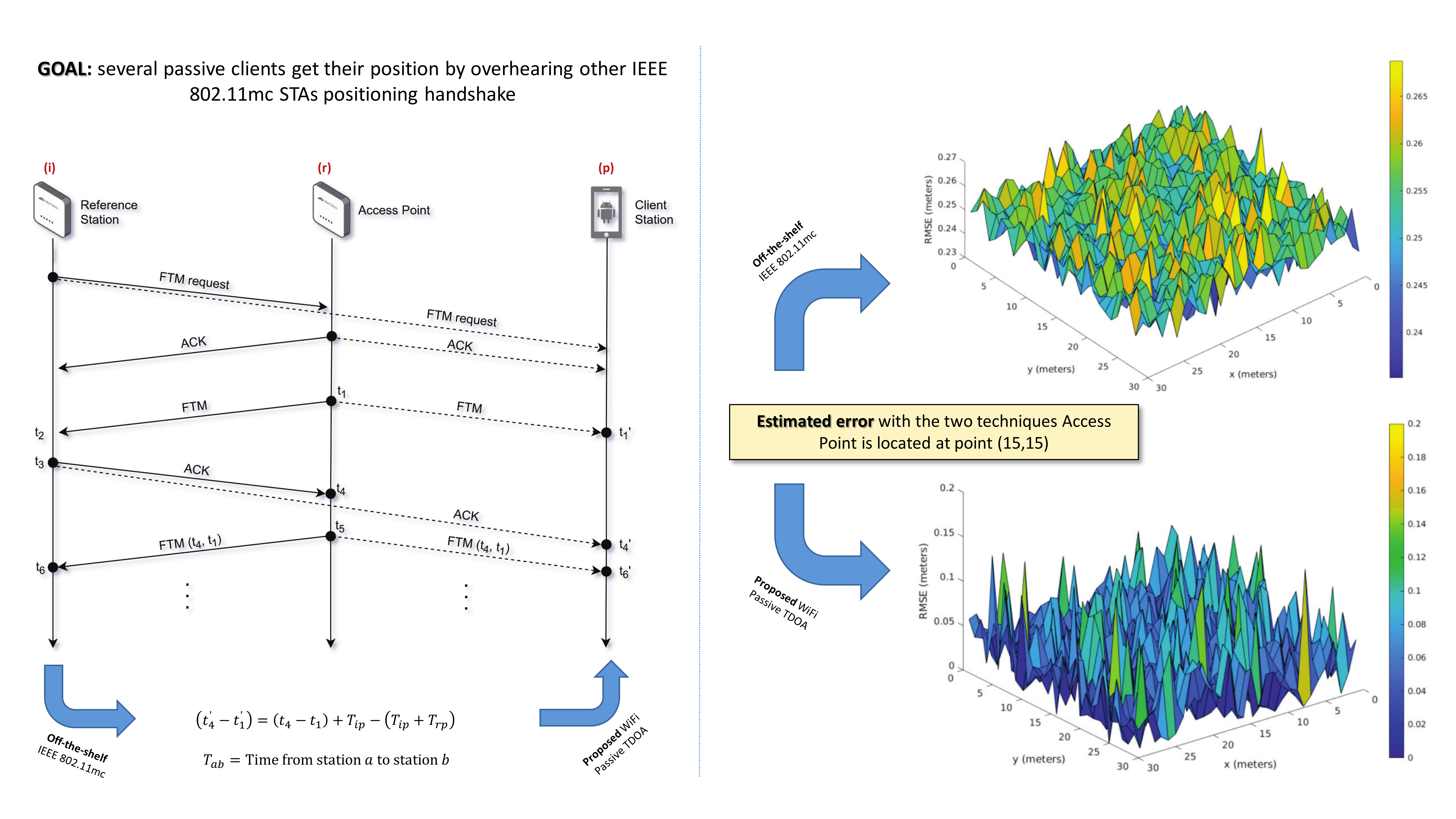
Details of the whole location process are depicted in
Figure 1. First, the initiating station begins a location session by sending an initial FTM request frame. The main goal of this message is setting up the parameters of the location procedure, including the number of bursts, the number of measurements per burst, the time between consecutive measurements, etc. Once the session is active, several FTMs need to be performed. To do so, the responding station sends an FTM frame and records the departure time of that frame (i.e.,
t1 in
Figure 1). After a while, this FTM frame will be received in the initiating station, which records the reception time (i.e.,
t2 in
Figure 1). An FTM frame needs to be confirmed by sending back an acknowledgement (ACK) frame. Accordingly, the initiating station responds with an ACK frame and records its departure time (i.e.,
t3 in
Figure 1). Eventually, the ACK frame is received in the responding station, which again records the reception time (i.e.,
t4 in
Figure 1). Finally, the timestamps
t1 and
t4 need to be reported back to the initiating station, where the position is actually going to be computed. This is achieved by running another FTM measurement (in the same burst or the next one) and including these timestamps as input data in the FTM frame being sent (e.g.,
FTM(t1,t4) in
Figure 1).
Once the initiating station receives
t1 and
t4 from the responding station, it could compute its position as follows:
RTTs can be subsequently turned into a distance as follows:
where
c is the propagation speed (i.e., the speed of light). This procedure must be repeated with at least three different responding stations for 2D positioning (four in the case of 3D positioning). Then, any regular multilateration algorithm could be used to fix the position. As in IEEE 802.11v, when responding stations are the APs, association with them is no longer required, which noticeably reduces the response time until the position is computed.
As shown in
Figure 1, the procedure proposed in IEEE 802.11mc consists of a peer-to-peer message exchange. A basic exchange such as the one depicted in
Figure 1 might spend approximately 30 ms, which means that under a tracking rate of 1 position per second, less than 34 devices could be served at once by a single AP. Furthermore, tracking such a number of location requests would mean no room for regular data traffic, which indeed is the main goal of IEEE 802.11 networks.
Accordingly, in order to achieve scalable time-based positioning solutions, passive location approaches should be further investigated, such as those where stations are able to determine their position without injecting location traffic.
5. WiFi Passive TDOA
5.1. The WiFi Passive TDOA Algorithm
IEEE 802.11mc provides a promising procedure for the native location in IEEE 802.11 networks; however, as the IEEE 802.11mc procedure needs location traffic to be injected (i.e., FTM-related frames), it does not scale well in future-dense scenarios where an increasing number of nodes is expected (e.g., IoT, 5G). A novel passive solution is proposed in this paper that combines the algorithm proposed in [
6] with the one proposed in IEEE 802.11mc [
5], so mobile stations (i.e., UEs) in the network can passively determine their own position without consuming the available data throughput for location purposes.
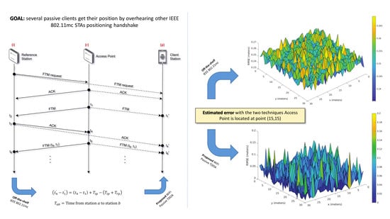
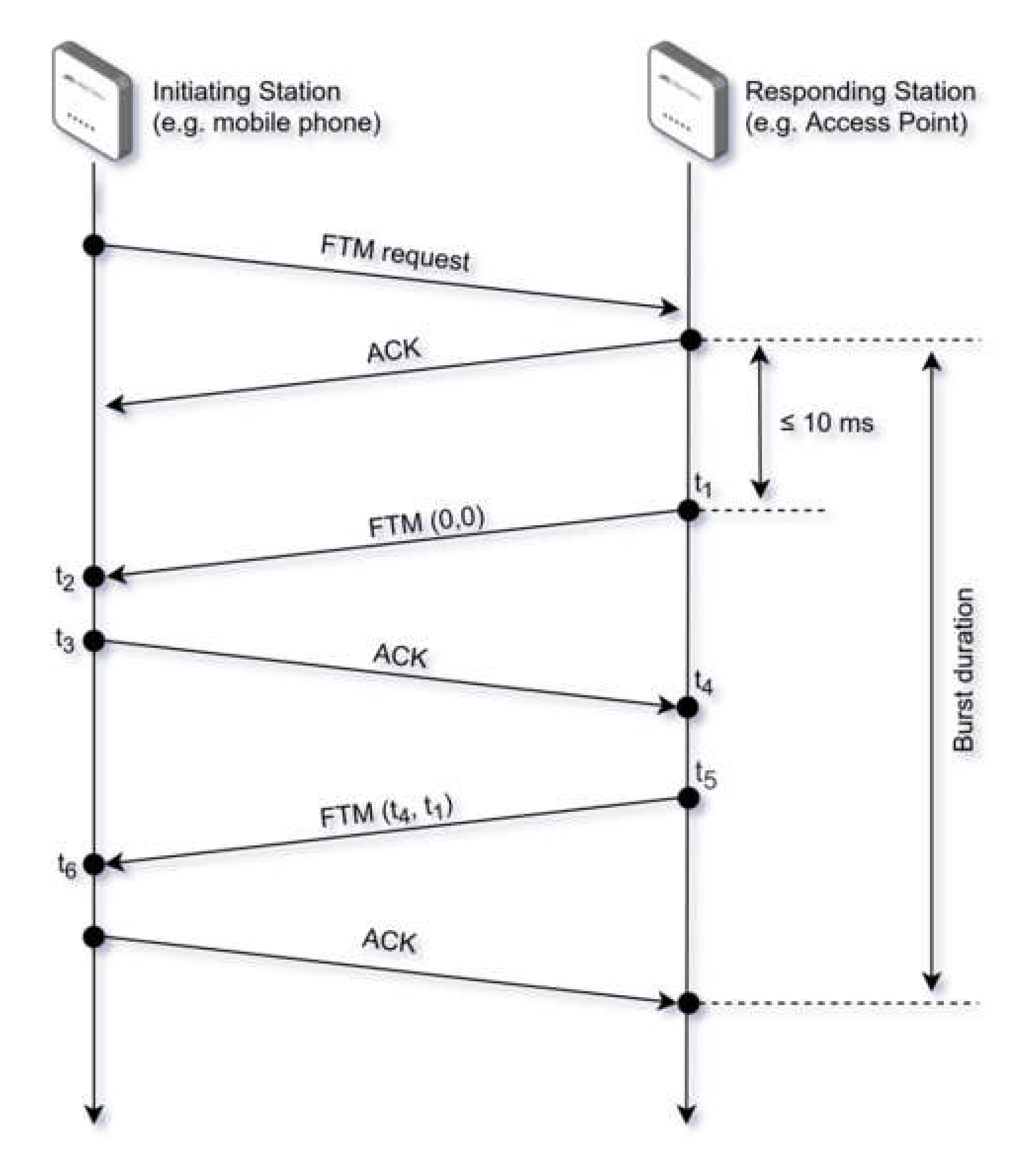
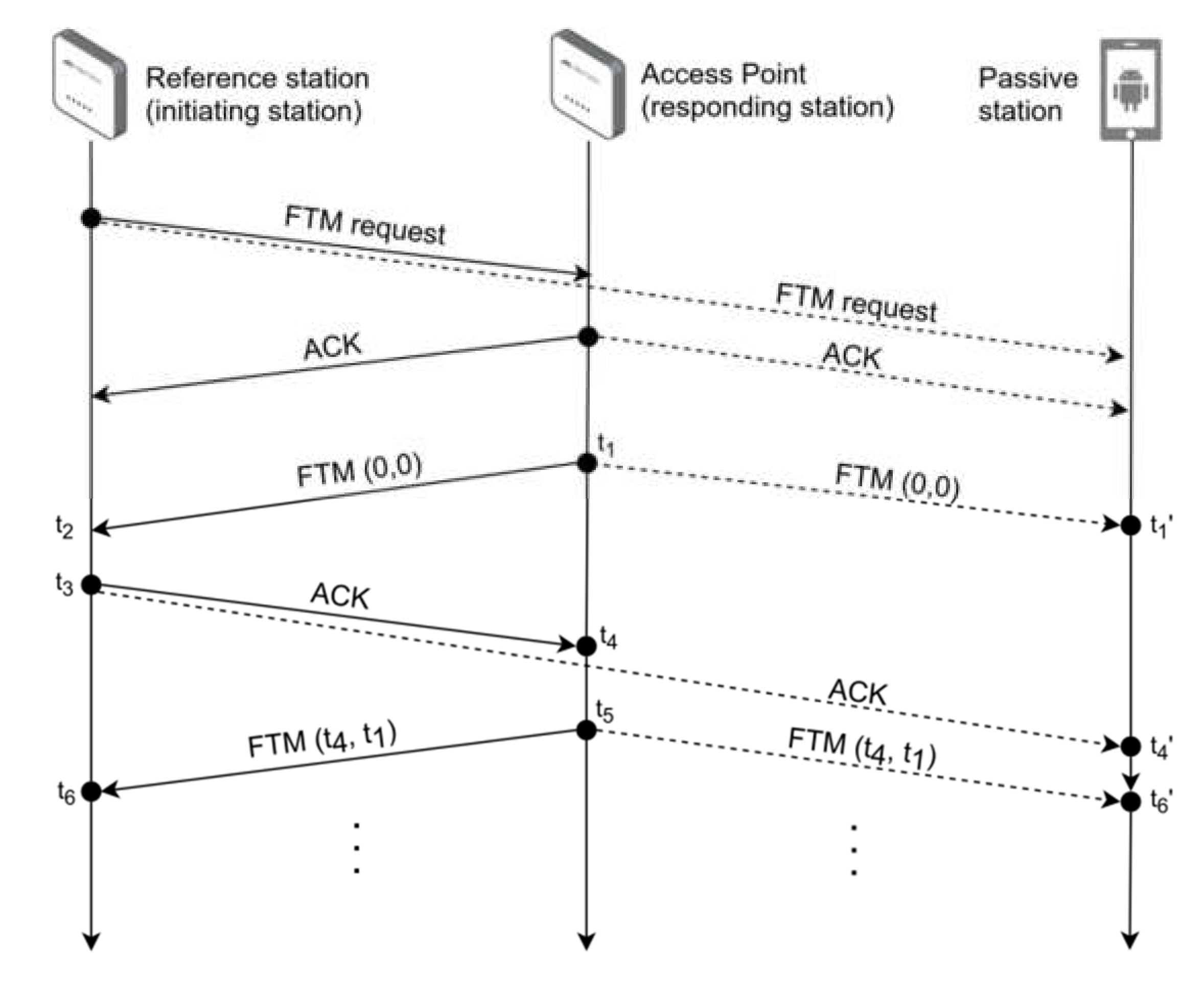
Figure 2 shows the flow of the
WiFi passive TDOA approach, resulting from merging the previously mentioned algorithms. Three stations are identified, including a reference station, a response station, and a passive station. The former represents a station that actively estimates the RTT using the IEEE 802.11mc procedure. The response station is the counterpart of the bouncing approach presented in IEEE 802.11mc (e.g., an AP in
Figure 2). Finally, the passive station is a mobile station that will listen to the frames being exchanged in the shared medium, and that will take advantage of them for calculating its own position.
Although it is not mandatory, no more than one reference station is expected to be involved in a location procedure, as additional location traffic would be injected otherwise. The remaining stations in the network (i.e., others than the reference and the response stations) are considered as passive stations. Without loss of generality and for the sake of simplicity, the explanation in this work considers one station of each kind.
As shown in
Figure 2, the process is ruled by the reference station, which corresponds to the initiating station in the IEEE 802.11mc procedure described in
Section 4. The reference station sends an FTM request frame that will be answered by the responding station with an ACK frame. Then, a pair of FTM and ACK frames are sent so the rough RTT (i.e.,
t4 -
t1) could be measured in the responding station. Finally, the timestamps involved in the rough RTT computation are reported back to the reference station, as described in IEEE 802.11mc. With all the timestamps in the reference station, the actual RTT could be computed, as shown in (1).
Due to the broadcast nature of the WiFi medium, all the frames exchanged between the reference and the responding stations will reach the passive station as well. We need the passive station to be listening to any FTM session setup in the network. Upon reception of the initial FTM request frame, the passive station will set up a precise time of arrival measurement (as done in the IEEE 802.11mc) on the reception of the next FTM frame and its corresponding ACK frame. This leads to timestamps and , respectively. Upon timestamping, all the frames will be silently discarded, as any other frame not addressed specifically to the passive station. When using the same clock to take two timestamps (i.e., and ), a time difference of arrival (TDOA) could be computed. This TDOA involves the following two paths: 1) from the responding station to the passive station and 2) from the responding station to the reference station, and then from there to the passive station. With a TDOA defining a hyperbola of possible positions, several FTM measurements activated by different responding stations (e.g., three or more for 2D positioning) are required so that the multilateration algorithms could be run, and a position for the passive station calculated. The following section shows how to build an equation system suitable for use by a multilateration algorithm.
5.2. Passive TDOA Formulation
Passive stations aim at measuring TDOAs from the IEEE 802.11mc traffic being exchanged in the network. The measured TDOA involves the following two paths: 1) from the responding station (i.e., the AP) to the passive station and 2) from the responding station to the reference (i.e., initiating) station, and from there to the passive station.
Timestamps t4 and t1, gathered in the responding station as a result of the RTT measurement process run by the initiating station, are included in the next FTM frame transmitted by the responding station. The time of arrival of the FTM frames is precisely measured at passive stations, and the timestamp data in the FTM frames (if present) are extracted before silently discarding the frames. Hence, t4 and t1 timestamps could be considered known at the passive station. The unknown timing is the one spent in the initiating station since an FTM frame, coming from the responding station, is received until the corresponding ACK frame is generated (i.e., t3 − t2); this variable is called δ.
The passive station can compute a rough RTT as follows:
In the following, how the passive station can infer
δ from other estimates is discussed. According to the flow shown in
Figure 2, the passive station can calculate a TDOA as follows:
where subscripts
i,
r, and
p stand for the initiating (reference) station (i.e., the active one), the responding station, and the passive station, respectively;
Tab is the TOF from station
a to station
b (e.g.,
Tri is the TOF from the responding station
r to the initiating station
i).
According to the proposed nomenclature, (3) can be written as follows:
Under the assumption of both TOF, from responding to initiating station and reversal, being equal, (5) yields the following:
The
δ value is only known at the initiating station; however, by adding and subtracting the term
Tri, (4) can be rewritten as follows:
Then, (6) and (7) can be merged as follows:
Considering
Figure 2, (8) could be understood as follows:
and then, grouping the time spent traversing each path in the TDOA, (9) can be rewritten as follows:
Equation (10) demonstrates that the only remaining unknowns are the position of the initiating and passive stations associated with the times
Tip,
Tir, and
Trp. Notice that these times are not estimated individually but are conceptually used in the ranging model to infer the position of both the active and passive stations. The ranging model is based on the following expression:
where
R(a,b) stands for the distance from the station
a to station
b;
c is the propagation speed (i.e., the speed of light), and
is the Euclidean norm applied to positions
and
, which are the position of the stations
a and
b, respectively. Equation (11) can be applied to (10) in order to turn the latter into a ranging model as follows:
where
Notice that
and the position of the responding station (
r) are known data at the passive station.
is computed at the passive station using the time measurements taken locally and the timestamps reported by the responding station to the initiating station. The initiating station (and hence the passive station) can obtain the position of the responding station by requesting the Location Information Configuration (LCI) or the Location Civic Report (LCR) [
5] during the ranging process, as long as the responding station supports such data structures. Otherwise, an out-of-band method (e.g., a local application) needs to be provided to supply the location of the involved responding stations.
Expanding ranges in (12), according to (11), leads to a nonlinear equation where the only unknowns are the position of both the active (
i) and passive (
p) stations.
Section 5.4 introduces some approaches that can be taken in order to infer both positions.
5.3. Error Estimation
Equation (10) defines the observed metric in passive stations under the assumption of no error. Under the presence of errors, (10) needs to be rewritten as follows:
where
etdoa and
ertt are the errors associated with the TDOA and the rough RTT measurements, respectively. Two conclusions could be raised from (14). The first one is that under similar propagation conditions, TDOA and rough RTT errors are expected to be the same, on average. Thus, on average, passive positions tend to have zero-mean errors.
Furthermore, under the assumption of no correlation between the rough RTT and TDOA measurements, the variance of the measurement error in the passive station becomes the sum of the variances of the rough RTT and TDOA measurements. Both rough RTT and TDOA are the result of time differences, as shown in (1) and (14), respectively. Thus, under the assumption that such time differences are independent and have identically distributed errors, measurements taken using both approaches (i.e., IEEE 802.11mc and WiFi passive TDOA) are expected to provide the same precision.
5.4. Joint Positioning
According to (10), at the passive station, two pieces of information need to be determined, including the position of the initiating (i.e., reference) station and the position of the passive station.
This joint positioning does not present an actual issue in network-based location systems, where stations do not use their own position information, but it is the network that tracks the position of all their devices. In this case, stations report the measurements to a location server in the network, which is in charge of computing all the positions. This is the scenario usually drawn by sensor networks such as those expected in IoT environments, which consists of humble devices unable to face the computational effort a position calculation requires [
27].
In the case of stations computing their own position, the passive station needs to know the position of the initiating station (e.g., through LCI/LCR) or otherwise be able to compute it. To overcome this issue, two approaches could be taken. The first approach could be to introduce a fixed initiating station at a known position, working as a landmark, and acting as part of the network infrastructure. Then, the position of the initiating station would be available to all the stations using the same approach applied to supply the positions of the responding stations, so that the passive stations could fix their own position from the measured TDOAs. This approach has the advantage of settling the initiating station in the best place in terms of both coverage and geometry. Thus, the expected accuracy of the computed positions might be maximized. Furthermore, for convenience, the initiating station duty could be integrated in one responding station (e.g., AP), different from the one used in the measurement process.
If the reference station cannot be part of the fixed network infrastructure, the passive station can still proceed with joint positioning as long as it has measurements coming from enough responding stations. According to Equation (12) and under the assumption that the responding station emplacements are known, there are only two unknowns remaining, the positions of the initiating and passive stations. Accordingly, the resulting equation system is:
where
n is the amount of responding stations involved in the joint positioning.
In this case, measurements from six different responding stations will be required for the 2D joint positioning (i.e., four unknowns for the coordinates and one extra equation to overcome the quadratic ambiguity for each position), whilst eight are required in the case of the 3D locations (i.e., the six coordinates to fix and two extra equations to remove the quadratic ambiguity). These measurements yield an overdetermined equation system in the initiating station when computing its own position and provide enough data in the passive station to jointly compute both the initiating and passive positions.
Whatever the solution taken for the joint positioning, the scalability of the location is ensured. Only one reference station is expected to inject location traffic (i.e., FTM) in a BSS, allocating the radio channel approximately 30 ms for each RTT measurement. In the worst case, when eight RTTs are required (i.e., involving eight different responding stations), it is expected that the reference station could gather enough information to compute its own position in less than 250 ms. Therefore, both periodical single location calls and continuous tracking would be possible in all the passive stations of the network. Furthermore, in the case of stations moving under pedestrian mobility patterns, taking 250 ms gathering data would involve an additional error in the order of a few centimeters, which would not limit the feasibility of the passive approach, especially when tracking algorithms (e.g., Extended Kalman Filter) are used.
6. Observed Time Error Assessment
6.1. Modeling the Measurement Error
Implementation of the WiFi passive TDOA in COTS devices requires access to the manufacturer firmware, which is often hard to obtain. Moreover, the evaluation may be biased by the specific manufacturer’s hardware, thus making it necessary to run the proposed approach on a large variety of devices in order to obtain a realistic and generic performance estimation. Therefore, simulation has been taken as a trade-off approach in assessing the performance of the WiFi passive TDOA algorithm. To this end, both the peer-to-peer IEEE 802.11mc and the WiFi passive TDOA procedures have been implemented in MATLAB R2019b.
The measurement error is one of the most noticeable sources of noise in ranging models, especially in the simplest models, as the one depicted in (11). Hence, the proposed simulation model is aimed at quantifying the measurement error expected from each of the approaches under real conditions, where measurement errors at reference and passive stations are expected to be correlated.
Measurement errors are modeled in MATLAB as additive noise to the actual time-of-flight (TOF) figures used to calculate both RTTs and TDOAs. The following two TOF error models have been considered—a Gaussian model and a distance-dependent model. The former provides Gaussian zero-mean errors (often used in positioning studies [
28]), with a standard deviation (
) of 10
−9 seconds. This figure means that 99.73% of the ranging errors computed according to (11) go below 1 meter.
Previous studies [
23], though, have reported that the further the station is from its access point, the less precise the measurement accuracy. Furthermore, preliminary experiments carried out by the authors on legacy terminals working with IEEE 802.11mc show that, below a certain distance threshold (i.e., 2–3 m), the closer the station is to its AP, the larger the ranging error and hence the larger the TOF estimation error. Accordingly, we have included a second zero-mean Gaussian model for the TOF error, in which the standard deviation is a function of the actual distance between the station and its AP, that is:
where
is the reference standard deviation (i.e., the same used in the regular Gaussian error model),
log computes the natural logarithm, and
d stands for the distance between the station and its AP. The constant
is used to make the function continuous.
The other main source of error on any position computation is the process noise, which depends on the dynamic model used for computing the positions and the technique used to do so. We must stress that the goal of this paper is to demonstrate the feasibility of the passive approach and to characterize the error magnitude that is expected in the measurement stage, compared with the current peer-to-peer approach. Addressing both measurement and process noise at the same time can encumber such a goal. Accordingly, and due to the length restrictions of this paper, assessing the positioning error is out of the scope of this work.
6.2. Simulation Scenario
The simulation scenario consists of a square-shaped area of 30 m × 30 m, with a single access point placed in the center, i.e., at (15,15). A one-meter-side grid has been drawn on the simulation surface. A reference station and a passive station (as defined in
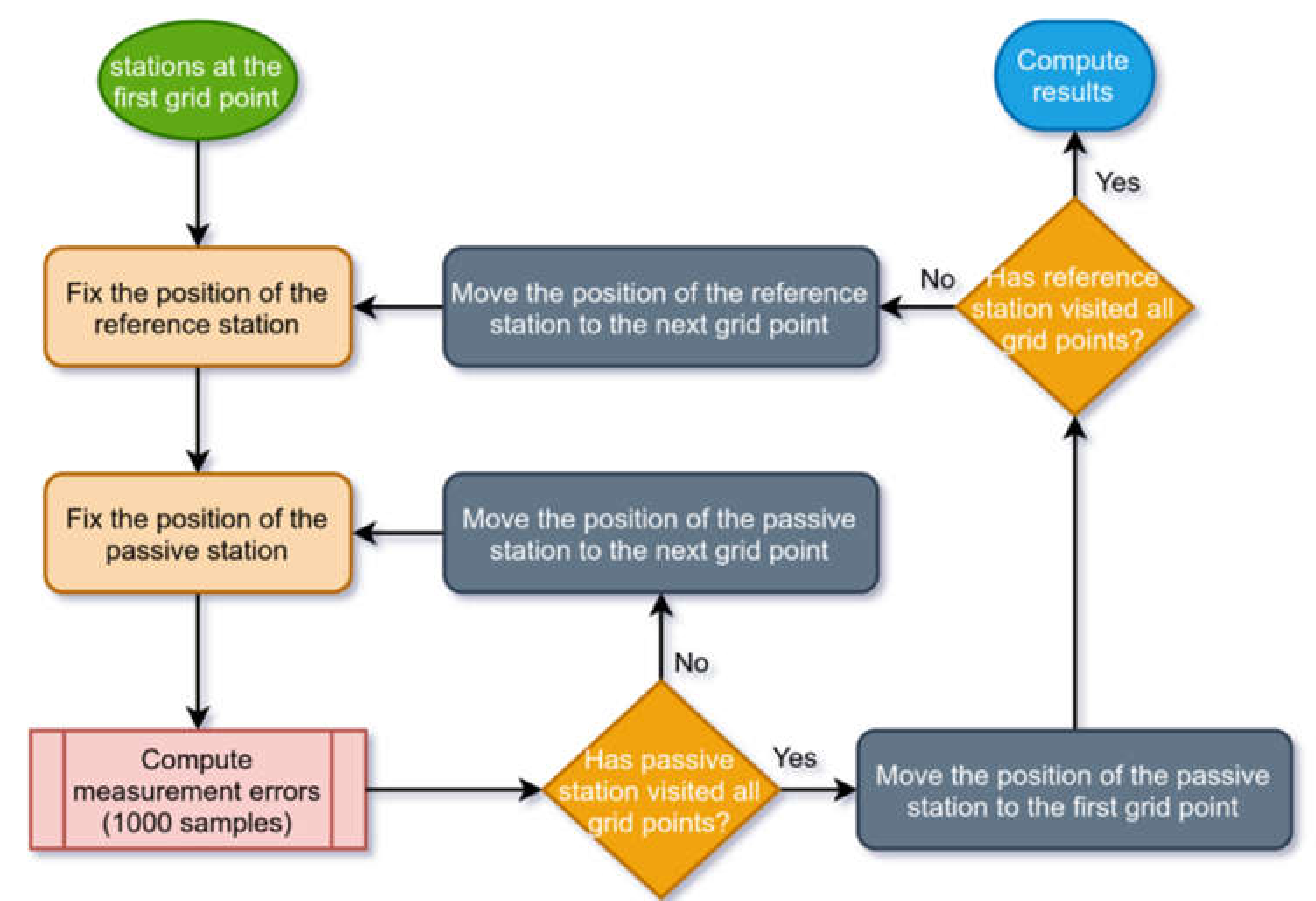
Section 5) are placed inside the grid. The methodology followed to gather the estimates is shown in
Figure 3 and is explained as follows:
Both the reference and passive stations are placed in the first point of the grid (i.e., the reference point (0, 0)).
The distances among the involved elements (i.e., the reference station, the AP and the passive station) are computed.
Time-of-flight errors are generated according to one of the two TOF error models and then applied to (1) and (14) in order to compute RTTs and TDOA errors, respectively. A sample of 1000 errors has been used here.
If the passive station has not yet visited all the points in the grid, it is moved to the next point, and the algorithm goes back to step 2. Otherwise, the passive station is moved to the reference point of the grid.
If the reference station has not yet visited all the points in the grid, it is moved to the next point, and the algorithm goes back to step 2.
Finally, the simulation is ended, and the statistics are computed.
6.3. Performance Assessment
The aim of this section is to prove the feasibility of the proposed WiFi Passive TDOA algorithm. To this end, we compare the expected measurement errors at passive stations (i.e., errors applied to TDOA measurements) with those reported when using the IEEE 802.11mc technique (i.e., errors applied to RTT measurements). This comparison is achieved by computing the measurement errors according to the methodology described in
Figure 3. The measurements errors are then turned into distance or distance-difference errors (by multiplying by the speed of light) in order to be better understood.
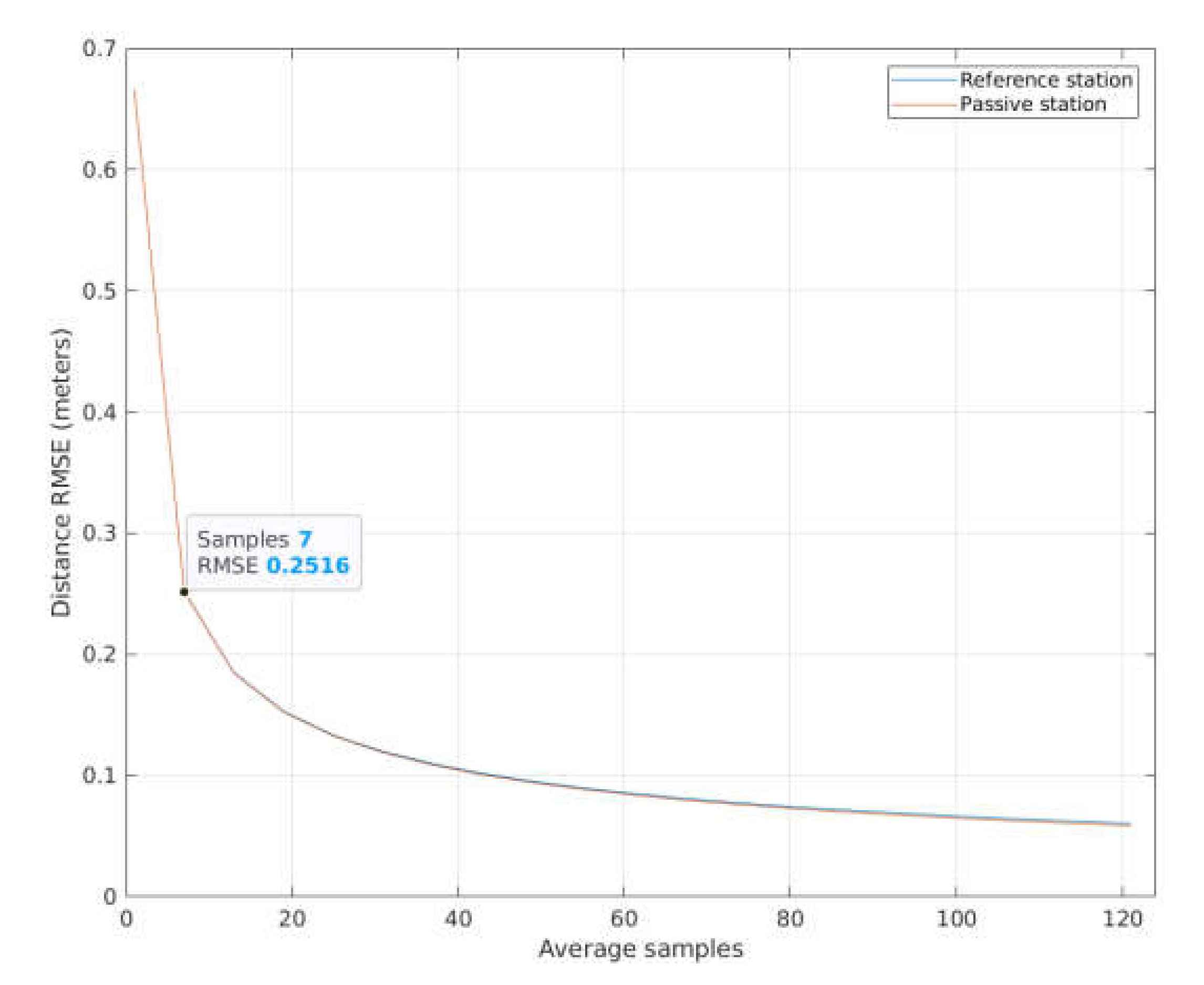
Figure 4 shows the average measurement root mean squared error (RMSE) in both techniques, IEEE 802.11mc, and WiFi Passive TDOA. This average is computed as follows. First, the measurement errors are grouped in sets of samples. Each sample set mimics the concept of burst in IEEE 802.11mc, which is a process that provides not a single but several RTT estimations for the same initiating and response station. Then, each sample set is averaged, which reduces the total amount of RTT estimations, as sample-set-size RTTs are used for a single averaged RTT estimation. Finally, the root mean square error (RMSE) of the averaged RTT estimations is computed. The procedure applies to the WiFi Passive TDOA, since this technique uses the messages generated by one station running the IEEE 802.11mc technique.
Any sample-set length could be used for computing the average RMSE; here, a sample set of length seven is used as a reference. This is because there are seven RTT samples gathered by the Android platform in a single burst when the IEEE 802.11mc technique is run on a mobile phone running such a platform.
In
Figure 4, sample sets from 1 to 121 are used. As shown, both IEEE 802.11mc, and WiFi Passive TDOA report almost the same RMSE values. This behavior is consistent with previous results (14), as explained in
Section 5. The confidence interval for the estimation is not depicted since it is below 0.25% of the average value.
Figure 5 shows in detail the average RMSE of the RTT measurement taken by the IEEE-802.11mc reference station, under the assumption of white Gaussian error noise on the time-of-flight measurements and a sample set of length seven. The RMSE figures move approximately 0.25 m. This value and the variability of the RMSE data are a consequence of the limited amount of data (i.e., 1000 error measurements) used for the computation of each measurement error sample.
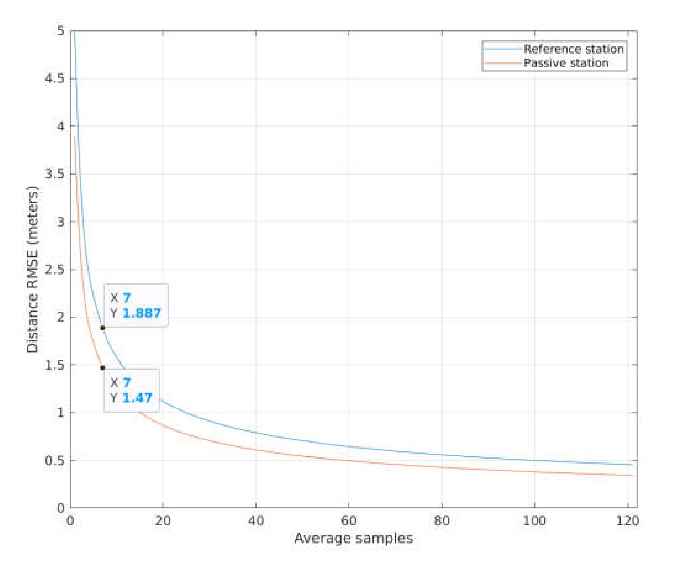
Figure 6 shows the average RMSE of both techniques when the distance-dependent error model in (16) is used. As shown, WiFi Passive TDOA provides better estimations regardless of the sample set length. This is because, according to Equation (16), short paths are especially impacted in terms of error. As the WiFi Passive TDOA involves two stations (i.e., initiating and passive STAs), it is unlikely that both of them draw very short paths to each other and with the responding station, resulting in better performance if compared with the RTTs estimated at the reference station (i.e., according to the legacy IEEE 802.11mc procedure). As shown in
Figure 4, the sample set of seven is used as a reference to compare both techniques. With this length, WiFi Passive TDOA shows a reduction of 22% in the average RMSE when compared with the results achieved by the IEEE 802.11mc technique.
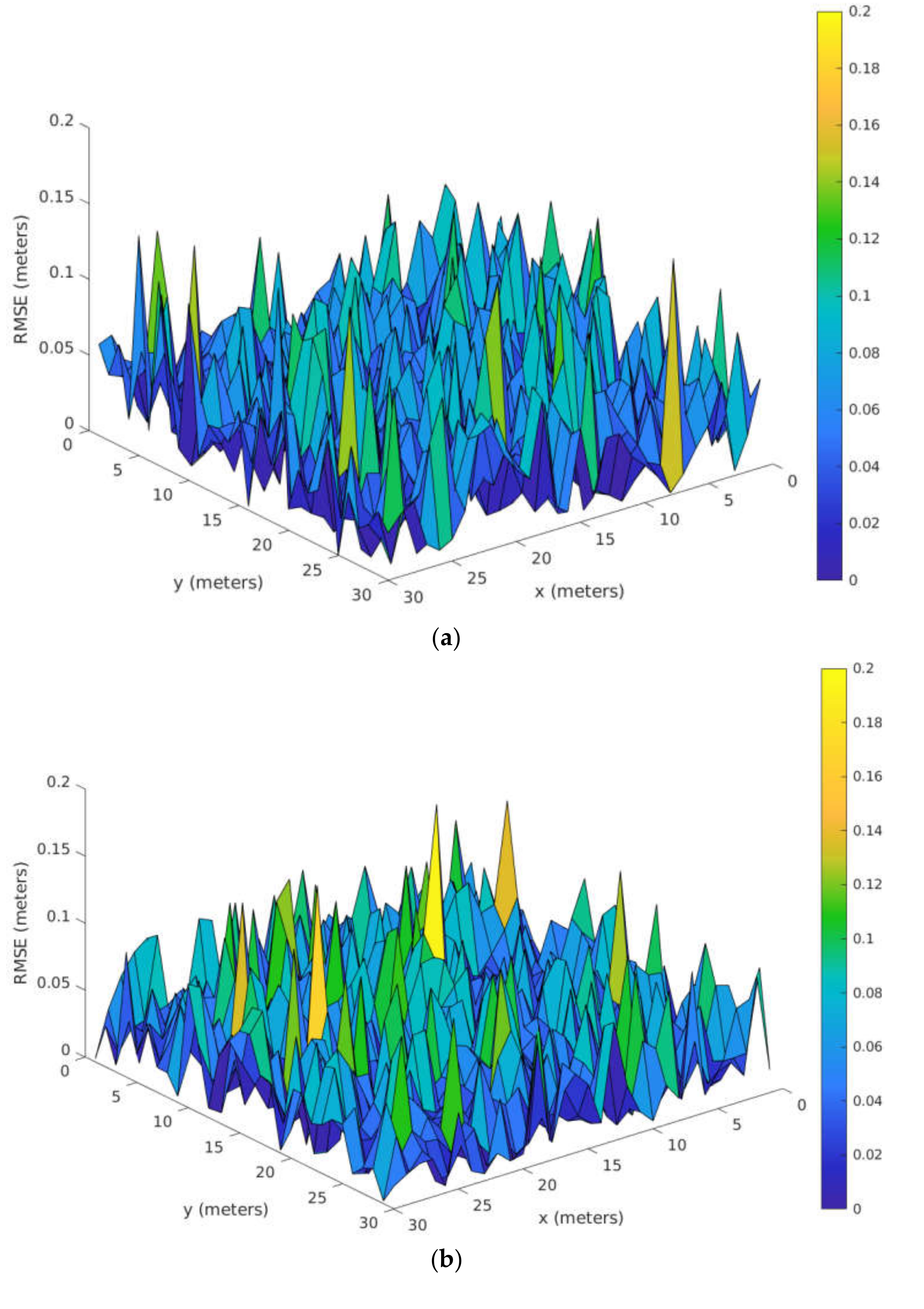
Figure 7 provides details of the data summarized in
Figure 6. Specifically,
Figure 7 displays the RMSE of the TDOA measurements taken at the passive station, when settled at each point of the grid. The reference sample set length is set to seven. Two cases are studied, depending on where the reference station is positioned, as follows: (a) at the top left corner (i.e., at point (1,1) in the grid) and (b) close to its AP (i.e., at point (14,14) in the grid). The former represents the case of good geometry, where the stations and the AP are rather far from each other most of the time. The latter depicts an example of poor geometry, in which at least one distance is noticeably shorter, and hence TDOA measurements are prone to involve measurement errors close to those reported at IEEE 802.11mc reference stations when the RTT is estimated. Furthermore, such short distances involve noticeable errors according to the model applied in (16). Data in
Figure 7 confirms this assumption, showing that in the case of poor geometry (i.e.,
Figure 7b), RMSE values are generally higher than those in the case of good geometry (i.e.,
Figure 7a), reaching up to 25% in the worst cases.
7. Conclusions and Future Work
Despite the volume of proposals available in the literature, specific research is still needed in order to define an indoor location algorithm that is able to provide high accuracy (i.e., under one meter) while being scalable with the increasing number of devices expected in the near future (i.e., IoT, 5G). This paper presents an algorithm called the
WiFi passive TDOA, which allows all stations in the network to be positioned passively at once. This is done by merging the following two techniques—RTT measurements defined in the IEEE 802.11mc standard [
5] and the algorithm presented in [
6]. The simulation results shown in this paper demonstrate that the WiFi passive TDOA algorithm provides good expectations in terms of scalability, precision, and response time.
However, several issues should be addressed in the future:
Tracking responding stations. The WiFi passive TDOA algorithm requires passive stations to listen to the location traffic exchanged by an active initiating station. This traffic involves several responding stations that are expected to work on different radio channels. Accordingly, either the passive stations scan those channels periodically to catch the location traffic or a scanning procedure should be set (e.g., basic service set identifiers (BSSIDs) visited in natural ascending order).
Overdetermined equation systems in reference stations. In the case of the joint-positioning of the reference and passive stations in the passive station, the reference station must measure many more RTTs than required for computing its own position. The number of measurements, as well as the responding stations used by the initiating station are decided at the application level, so this is an easy issue to address.
Dual active-passive role. Passive stations rely on one reference station being at sight; otherwise, the passive station cannot fix its position. A dual active-passive role is to be defined in the passive stations so they can overcome this issue and run a regular IEEE 802.11mc location process when the passive approach is not feasible.
Firmware upgrade. Although the presented algorithm is based on the frames and procedures defined in the IEEE 802.11mc standard, passive stations need to listen to traffic that is not addressed to them. This behavior requires slight modifications in the firmware of wireless interface cards so that passive stations do not discard FTM frames, even if they are not addressed to them until the measurements are made. The support of a network manufacturer or a development kit being available is required to move the technology to actual devices.
Security issues. Although security issues are out of the scope of this paper, passive node processing frames not being addressed to them might raise security issues that should be addressed.
Performance assessment. A wider performance assessment on measurement errors should be carried out. For instance, process errors need to be studied by providing a dynamic model and assessing several approaches for position computation (e.g., iterative nonlinear positioning, tracking algorithms, etc.). Furthermore, other performance parameters, such as the response time, scalability, sensitivity to network failures (e.g., link-layer collisions), etc., need to be addressed as well. Therefore, full network-stack simulations and implementations on actual devices will be carried out in the near future to corroborate the expected performance of the proposed algorithm.


