Automated Data Acquisition System Using a Neural Network for Prediction Response in a Mode-Locked Fiber Laser


 , ,
, ,  and
and 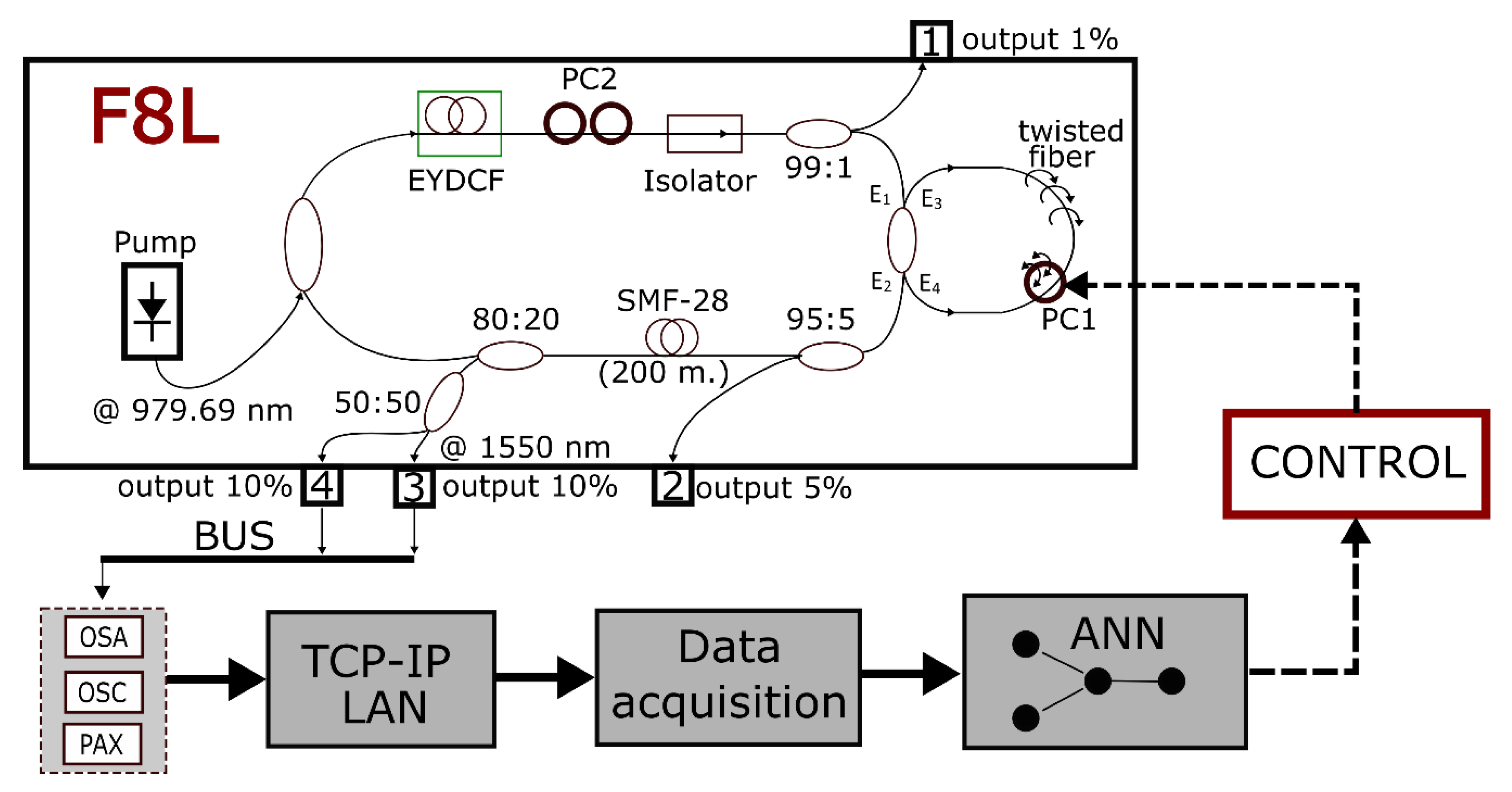
Abstract
1. Introduction
2. Materials and Methods
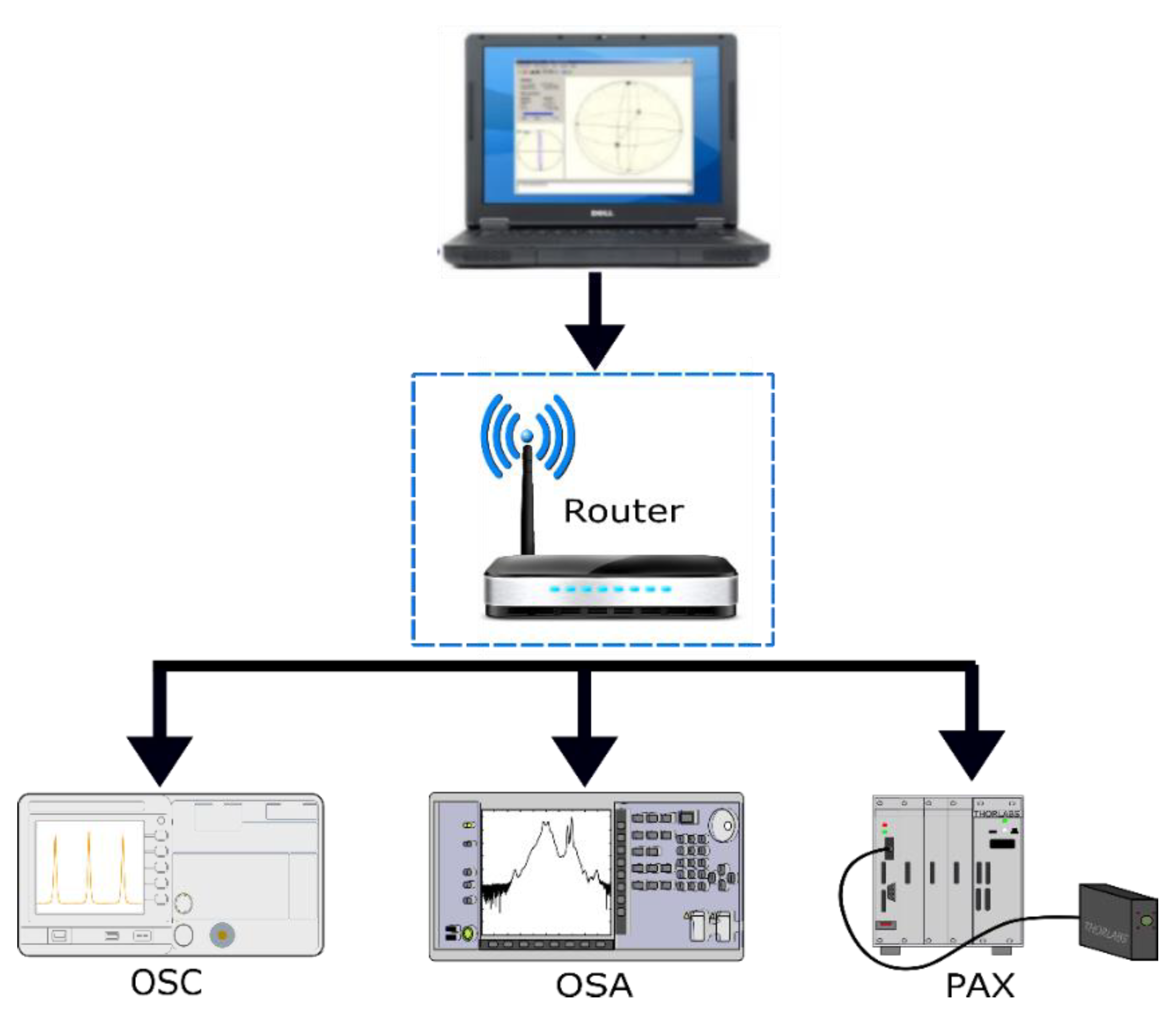
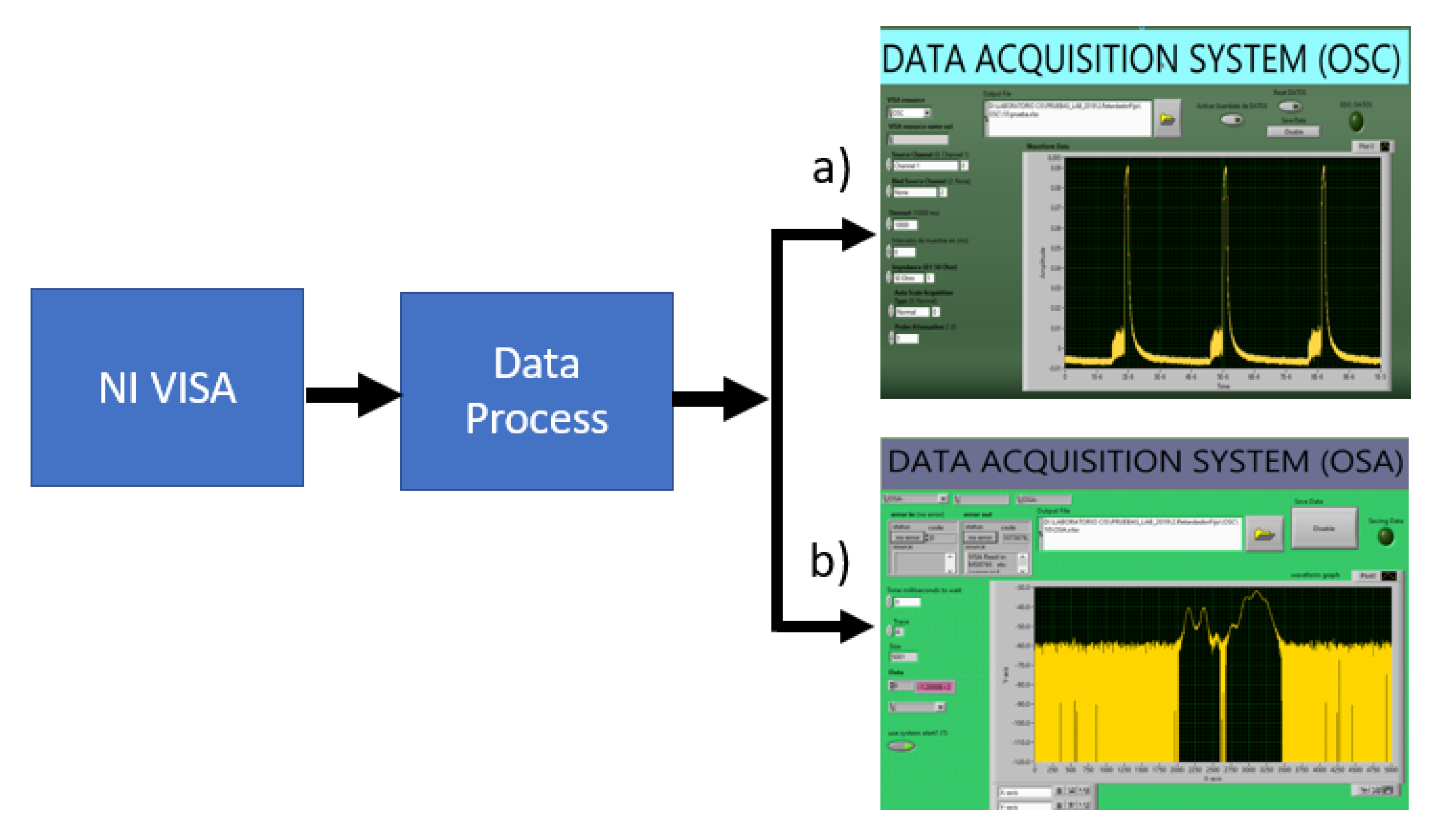
2.1. Laser Setup and Data Handling
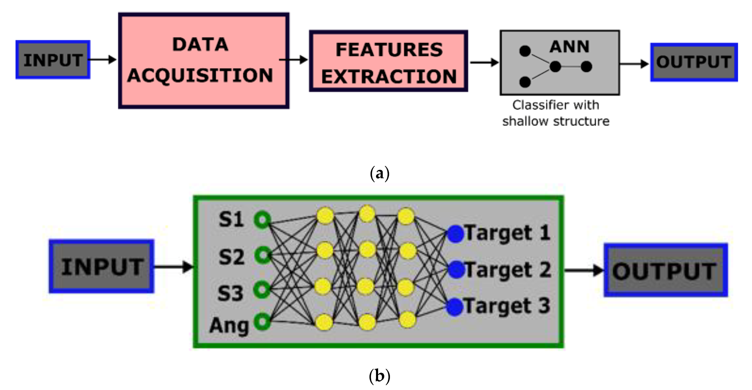
2.2. Artificial Neural Networks (ANN)
3. Results
4. Conclusions
Author Contributions
Funding
Acknowledgments
Conflicts of Interest
References
- De Georgia, M.A.; Kaffashi, F.; Jacono, F.J.; Loparo, K.A. Information technology in critical care: Review of monitoring and data acquisition systems for patient care and research. Sci. World J. 2015, 2015, 1–9. [Google Scholar] [CrossRef] [PubMed]
- Costas-Perez, L.; Lago, D.; Farina, J.; Rodriguez-Andina, J.J. Optimization of an industrial sensor and data acquisition laboratory through time sharing and remote access. IEEE Trans. Ind. Electron. 2008, 55, 2397–2404. [Google Scholar] [CrossRef]
- Schumacher, P.M. Data Acquisition System for Large Format Video Display. U.S. Patents 4485409, 27 November 1984. [Google Scholar]
- Michelon, G.K.; Bazzi, C.L.; Upadhyaya, S.; de Souza, E.G.; Magalhães, P.S.G.; Borges, L.F.; Schenatto, K.; Sobjak, R.; Gavioli, A.; Betzek, N.M. Software AgDataBox-Map to precision agriculture management. SoftwareX 2019, 10, 100320. [Google Scholar] [CrossRef]
- Patena, G.; Ingram, K.T. Digital acquisition and measurement of peanut root minirhizotron images. Agron. J. 2000, 92, 541–544. [Google Scholar] [CrossRef]
- Ameur, S.; Laghrouche, M.; Adane, A. Monitoring a greenhouse using a microcontroller-based meteorological data-acquisition system. Renew. Energy 2001, 24, 19–30. [Google Scholar] [CrossRef]
- Kumar, N.P.A.; Jagadeesh Chandra, A.P. Development of Remote Instrumentation and Control for Laboratory Experiments using Handheld Devices. Int. J. Online Biomed. Eng. iJOE 2019, 15, 31–43. [Google Scholar]
- Sanders, J.W.; Fletcher, J.R.; Frank, S.J.; Liu, H.-L.; Johnson, J.M.; Zhou, Z.; Chen, H.S.-M.; Venkatesan, A.M.; Kudchadker, R.J.; Pagel, M.D.; et al. Deep learning application engine (DLAE): Development and integration of deep learning algorithms in medical imaging. SoftwareX 2019, 10, 100347. [Google Scholar] [CrossRef]
- Binder, J.M.; Stark, A.; Tomek, N.; Scheuer, J.; Frank, F.; Jahnke, K.D.; Müller, C.; Schmitt, S.; Metsch, M.H.; Unden, T.; et al. Qudi: A modular python suite for experiment control and data processing. SoftwareX 2017, 6, 85–90. [Google Scholar] [CrossRef]
- Nguyen, D.T.; Kaneshiro, B. AudExpCreator: A GUI-based Matlab tool for designing and creating auditory experiments with the Psychophysics Toolbox. SoftwareX 2018, 7, 328–334. [Google Scholar] [CrossRef]
- Tian, H.; Wang, T.; Liu, Y.; Qiao, X.; Li, Y. Computer vision technology in agricultural automation—A review. Inf. Process. Agric. 2019. [Google Scholar] [CrossRef]
- Suk, H.-J.; Boyden, E.S.; van Welie, I. Advances in the automation of whole-cell patch clamp technology. J. Neurosci. Methods 2019, 326, 108357. [Google Scholar] [CrossRef] [PubMed]
- Chen, X.; Song, G.; Zhang, Y. Virtual and remote laboratory development: A review. In Earth and Space 2010: Engineering, Science, Construction, and Operations in Challenging Environments; ASCE: Reston, VA, USA, 2010. [Google Scholar] [CrossRef]
- Elliott, C.; Vijayakumar, V.; Zink, W.; Hansen, R. National Instruments LabVIEW: A Programming Environment for Laboratory Automation and Measurement. JALA J. Assoc. Lab. Autom. 2007, 12, 17–24. [Google Scholar] [CrossRef]
- Liu, L.G.; Li, J.H.; Deng, L.H. Design of data acquisition system based on labVIEW. Adv. Mater. Res. 2012, 569, 808–813. [Google Scholar] [CrossRef]
- Liao, H.; Qiu, Z.; Feng, G. The design of LDF data acquisition system based on LabVIEW. Procedia Environ. Sci. 2011, 10, 1188–1192. [Google Scholar] [CrossRef]
- Hunter, P. The advent of AI and deep learning in diagnostics and imaging. EMBO Rep. 2019, 20, e48559. [Google Scholar] [CrossRef]
- Chakravarty, A.; Mentink, J.; Davies, C.; Yamada, K.; Kimel, A.; Rasing, T. Supervised learning of an opto-magnetic neural network with ultrashort laser pulses. Appl. Phys. Lett. 2019, 114, 192407. [Google Scholar] [CrossRef]
- Boutaba, R.; Salahuddin, M.A.; Limam, N.; Ayoubi, S.; Shahriar, N.; Estrada-Solano, F.; Caicedo, O.M. A comprehensive survey on machine learning for networking: Evolution, applications and research opportunities. J. Internet Serv. Appl. 2018, 9, 16. [Google Scholar] [CrossRef]
- Ghaheri, A.; Shoar, S.; Naderan, M.; Hoseini, S.S. The applications of genetic algorithms in medicine. Oman Med. J. 2015, 30, 406. [Google Scholar] [CrossRef] [PubMed]
- Szeliski, R. Computer Vision: Algorithms and Applications; Springer Science & Business Media: London, UK, 2010. [Google Scholar]
- Koljonen, J.; Nordling, T.E.M.; Alander, J.T. A review of genetic algorithms in near infrared spectroscopy and chemometrics: Past and future. J. Near Infrared Spectrosc. 2008, 16, 189–197. [Google Scholar] [CrossRef]
- Woodward, R.I.; Kelleher, E.J.R. Towards ‘smart lasers’: Self-optimisation of an ultrafast pulse source using a genetic algorithm. Sci. Rep. 2016, 6, 37616. [Google Scholar] [CrossRef]
- Andral, U.; Fodil, R.S.; Amrani, F.; Billard, F.; Hertz, E.; Grelu, P. Fiber laser mode locked through an evolutionary algorithm. Optica 2015, 2, 275–278. [Google Scholar] [CrossRef]
- Kokhanovskiy, A.; Bednyakova, A.; Kuprikov, E.; Ivanenko, A.; Dyatlov, M.; Lotkov, D.; Kobtsev, S.; Turitsyn, S. Machine learning-based pulse characterization in figure-eight mode-locked lasers. Opt. Lett. 2019, 44, 3410–3413. [Google Scholar] [CrossRef]
- Hoffmann, A.; Zuerch, M.; Spielmann, C. Extremely nonlinear optics using shaped pulses spectrally broadened in an argon- or sulfur hexafluoride-filled hollow-core fiber. Appl. Sci. 2015, 5, 1310–1322. [Google Scholar] [CrossRef]
- Lu, H.; Xu, H.; Zhao, J.; Hou, D. A deep ultraviolet mode-locked laser based on a neural network. Sci. Rep. 2020, 10, 116. [Google Scholar] [CrossRef] [PubMed]
- Zimmermann, J.; Langbehn, B.; Cucini, R.; Di Fraia, M.; Finetti, P.; LaForge, A.C.; Nishiyama, T.; Ovcharenko, Y.; Piseri, P.; Plekan, O.; et al. Deep neural networks for classifying complex features in diffraction images. Phys. Rev. E 2019, 99, 063309. [Google Scholar] [CrossRef] [PubMed]
- Arteaga-Sierra, F.; Milián, C.; Torres-Gómez, I.; Torres-Cisneros, M.; Plascencia-Mora, H.; Moltó, G.; Ferrando, A. Optimization for maximum Raman frequency conversion in supercontinuum sources using genetic algorithms. Revista Mexicana de Física 2017, 63, 111–116. [Google Scholar]
- Arteaga-Sierra, F.; Milian, C.; Torres, I.; Torres-Cisneros, M.; Moltó, G.; Ferrando, A. Supercontinuum optimization for dual-soliton based light sources using genetic algorithms in a Grid platform. Opt. Express 2014, 22, 23686. [Google Scholar] [CrossRef]
- Ibarra-Escamilla, B.; Kuzin, E.; Duran-Sanchez, M.; Pottiez, O.; Haus, J. Symmetric nonlinear optical loop mirror used as saturable absorber in mode-locked fiber laser. In Proceedings of the Latin America Optics and Photonics Conference, Cancun, Mexico, 16–21 November 2014; p. LTu1A-3. [Google Scholar]
- Avazpour, M.; Beltrán-Pérez, G.; Rodríguez-Morales, L.A.; Armas-Rivera, I.; Ibarra-Escamilla, B.; Muñoz-Aguirre, S.; Castillo-Mixcóatl, J.; Pottiez, O.; Kuzin, E.A. The use of polarization-imbalanced NOLM to improve the quality of the spectrum compression. Opt. Laser Technol. 2019, 120, 105692. [Google Scholar] [CrossRef]
- Kashi, A.S.; Zhuge, Q.; Cartledge, J.C.; Etemad, S.A.; Borowiec, A.; Charlton, D.W.; Laperle, C.; Sullivan, M.O. Nonlinear signal-to-noise ratio estimation in coherent optical fiber transmission systems using artificial neural networks. J. Lightw. Technol. 2018, 36, 5424–5431. [Google Scholar] [CrossRef]
- Badhwar, P.; Kumar, A.; Yadav, A.; Kumar, P.; Siwach, R.; Chhabra, D.; Dubey, K.K. Improved pullulan production and process optimization using novel GA–ANN and GA–ANFIS hybrid statistical tools. Biomolecules 2020, 10, 124. [Google Scholar] [CrossRef]
- Nasser, I.M.; Abu-Naser, S.S. Predicting tumor category using artificial neural networks. Int. J. Acad. Health Med. Res. 2019, 3, 1–7. [Google Scholar]
- Izgi, E.; Öztopal, A.; Yerli, B.; Kaymak, M.K.; Şahin, A.D. Short-mid-term solar power prediction by using artificial neural networks. Sol. Energy 2012, 86, 725–733. [Google Scholar] [CrossRef]
- Olivier, M.; Gagnon, M.-D.; Piché, M. Automated mode locking in nonlinear polarization rotation fiber lasers by detection of a discontinuous jump in the polarization state. Opt. Express 2015, 23, 6738–6746. [Google Scholar] [CrossRef]
- Herrmann, I.; Berenstein, M.; Paz-Kagan, T.; Sade, A.; Karnieli, A. Spectral assessment of two-spotted spider mite damage levels in the leaves of greenhouse-grown pepper and bean. Biosyst. Eng. 2017, 157, 72–85. [Google Scholar] [CrossRef]
- Barrientos, F.; Ríos, S.A. Aplicación de minería de datos para predecir fuga de clientes en la industria de las telecomunicaciones. Revista Ingeniería de Sistemas 2013, 27, 73–107. [Google Scholar]
- Rumpf, T.; Mahlein, A.-K.; Steiner, U.; Oerke, E.-C.; Dehne, H.-W.; Plümer, L. Early detection and classification of plant diseases with support vector machines based on hyperspectral reflectance. Comput. Electron. Agric. 2010, 74, 91–99. [Google Scholar] [CrossRef]
- Schaefer, B.; Collett, E.; Smyth, R.; Barrett, D.; Fraher, B. Measuring the Stokes polarization parameters. Am. J. Phys. 2007, 75, 163–168. [Google Scholar] [CrossRef]
- Hernandez-Garcia, J.C.; Estudillo-Ayala, J.M.; Pottiez, O.; Filoteo-Razo, J.D.; Lauterio-Cruz, J.P.; Sierra-Hernandez, J.M.; Rojas-Laguna, R. Flat supercontinuum generation by a F8L in high-energy harmonic noise-like pulsing regime. Laser Phys. Lett. 2016, 13, 125104. [Google Scholar] [CrossRef]
- Ardalan, S.H.; Van Den Bout, D.E. Remote Access to Electronic Meters Using a TCP/IP Protocol Suite. U.S. Patent 0218616 A1, 4 November 2004. [Google Scholar]
- Vizcaíno, J.R.L.; Sebastiá, J.P. LabVIEW: Entorno Gráfico de Programación; Marcombo: Barcelona, Spain, 2011. [Google Scholar]
- Agrawal, G.P. Nonlinear Fiber Optics, 5th ed.; Academic Press: NewYork, NY, USA, 2013; p. 648. [Google Scholar]
- Ibrahimy, M.I.; Ahsan, R.; Khalifa, O.O. Design and optimization of Levenberg-Marquardt based neural network classifier for EMG signals to identify hand motions. Meas. Sci. Rev. 2013, 13, 142–151. [Google Scholar] [CrossRef]
- Tabet, M.F.; McGahan, W.A. Use of artificial neural networks to predict thickness and optical constants of thin films from reflectance data. Thin Solid Films 2000, 370, 122–127. [Google Scholar] [CrossRef]
- Liehr, S.; Jäger, L.A.; Karapanagiotis, C.; Münzenberger, S.; Kowarik, S. Real-time dynamic strain sensing in optical fibers using artificial neural networks. Opt. Express 2019, 27, 7405–7425. [Google Scholar] [CrossRef] [PubMed]
- Mohamad, N.; Zaini, F.; Johari, A.; Yassin, I.; Zabidi, A. Comparison between Levenberg-Marquardt and Scaled Conjugate Gradient training algorithms for Breast Cancer Diagnosis using MLP. In Proceedings of the 6th International Colloquium on Signal Processing & its Applications, Malacca City, Malaysia, 21–23 May 2010; pp. 1–7. [Google Scholar]
- Du, Y.-C.; Stephanus, A. Levenberg-Marquardt neural network algorithm for degree of arteriovenous fistula stenosis classification using a dual optical photoplethysmography sensor. Sensors 2018, 18, 2322. [Google Scholar] [CrossRef] [PubMed]
- Mohammed, R.K. Comparing various channel estimation techniques for OFDM systems using MATLAB. Int. J. Wirel. Mob. Netw. IJWMN 2019, 11. [Google Scholar] [CrossRef]


© 2020 by the authors. Licensee MDPI, Basel, Switzerland. This article is an open access article distributed under the terms and conditions of the Creative Commons Attribution (CC BY) license (http://creativecommons.org/licenses/by/4.0/).
Share and Cite
Martinez-Angulo, J.R.; Perez-Careta, E.; Hernandez-Garcia, J.C.; Marquez-Figueroa, S.; Barron Zambrano, J.H.; Jauregui-Vazquez, D.; Filoteo-Razo, J.D.; Lauterio-Cruz, J.P.; Pottiez, O.; Estudillo-Ayala, J.M.; et al. Automated Data Acquisition System Using a Neural Network for Prediction Response in a Mode-Locked Fiber Laser. Electronics 2020, 9, 1181. https://doi.org/10.3390/electronics9081181
Martinez-Angulo JR, Perez-Careta E, Hernandez-Garcia JC, Marquez-Figueroa S, Barron Zambrano JH, Jauregui-Vazquez D, Filoteo-Razo JD, Lauterio-Cruz JP, Pottiez O, Estudillo-Ayala JM, et al. Automated Data Acquisition System Using a Neural Network for Prediction Response in a Mode-Locked Fiber Laser. Electronics. 2020; 9(8):1181. https://doi.org/10.3390/electronics9081181
Chicago/Turabian StyleMartinez-Angulo, Jose Ramon, Eduardo Perez-Careta, Juan Carlos Hernandez-Garcia, Sandra Marquez-Figueroa, Jose Hugo Barron Zambrano, Daniel Jauregui-Vazquez, Jose David Filoteo-Razo, Jesus Pablo Lauterio-Cruz, Olivier Pottiez, Julian Moises Estudillo-Ayala, and et al. 2020. "Automated Data Acquisition System Using a Neural Network for Prediction Response in a Mode-Locked Fiber Laser" Electronics 9, no. 8: 1181. https://doi.org/10.3390/electronics9081181
APA StyleMartinez-Angulo, J. R., Perez-Careta, E., Hernandez-Garcia, J. C., Marquez-Figueroa, S., Barron Zambrano, J. H., Jauregui-Vazquez, D., Filoteo-Razo, J. D., Lauterio-Cruz, J. P., Pottiez, O., Estudillo-Ayala, J. M., & Rojas-Laguna, R. (2020). Automated Data Acquisition System Using a Neural Network for Prediction Response in a Mode-Locked Fiber Laser. Electronics, 9(8), 1181. https://doi.org/10.3390/electronics9081181