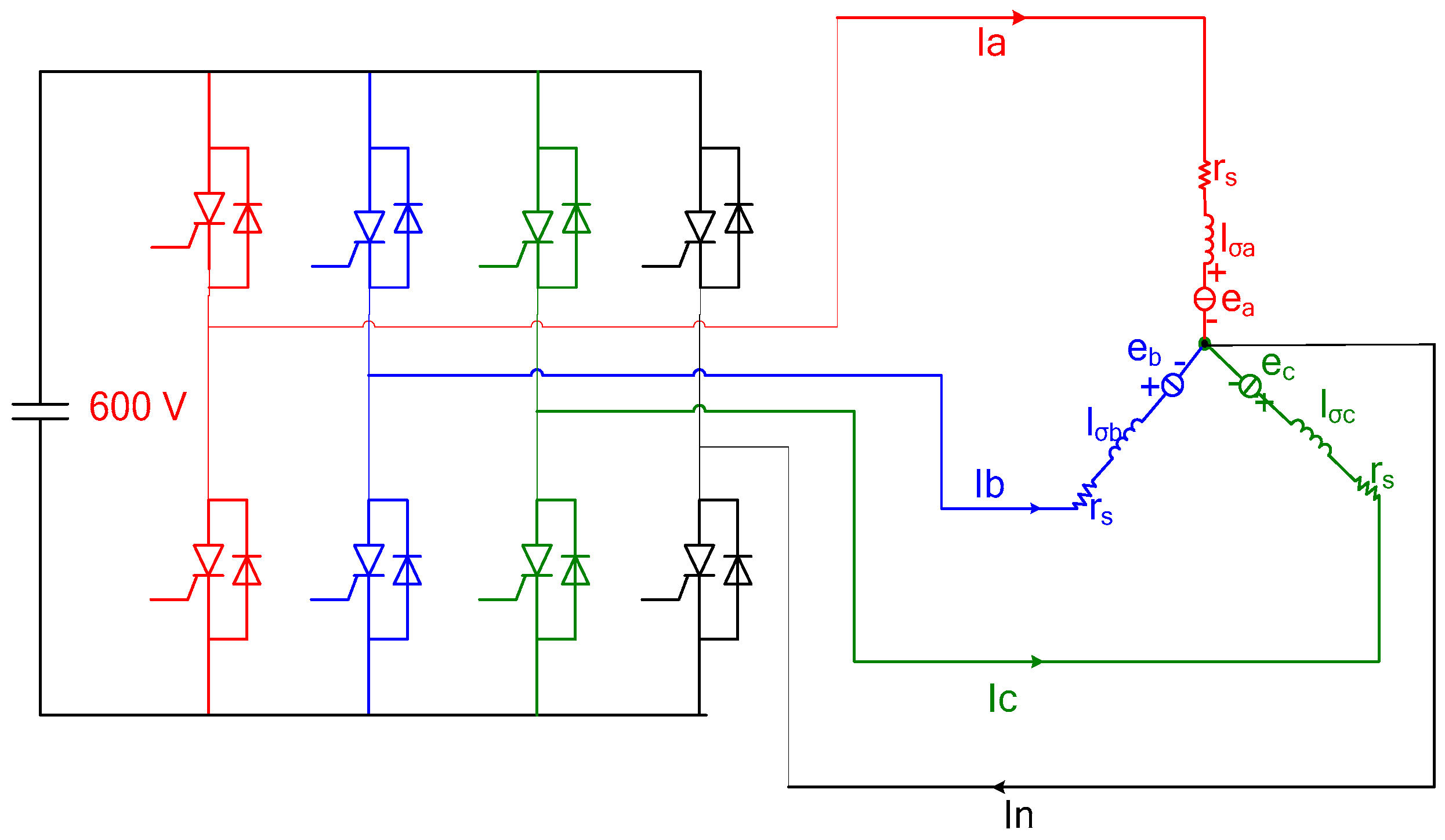
Figure 1.
Four-leg permanent magnet synchronous motors (PMSM) drive.
Figure 1.
Four-leg permanent magnet synchronous motors (PMSM) drive.
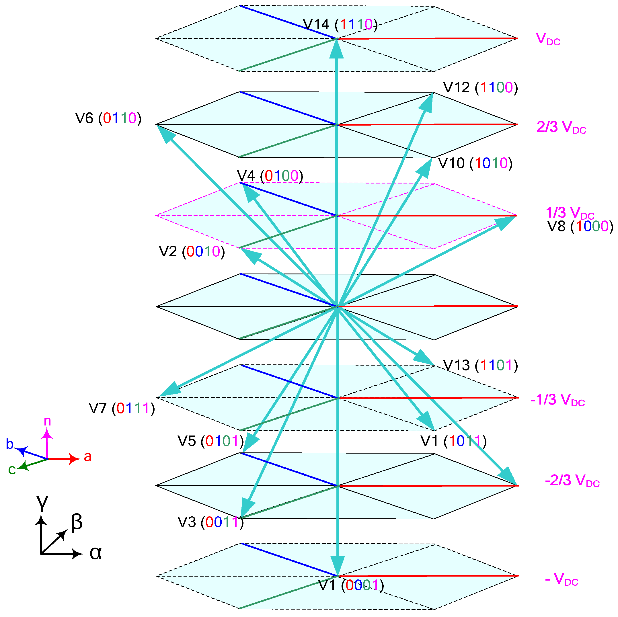
Figure 2.
Three-dimension space vector pulse width modulation (3D-SVPWM) for a four-leg inverter.
Figure 2.
Three-dimension space vector pulse width modulation (3D-SVPWM) for a four-leg inverter.
Figure 3.
The algorithm of the 3D-SPVPWM.
Figure 3.
The algorithm of the 3D-SPVPWM.
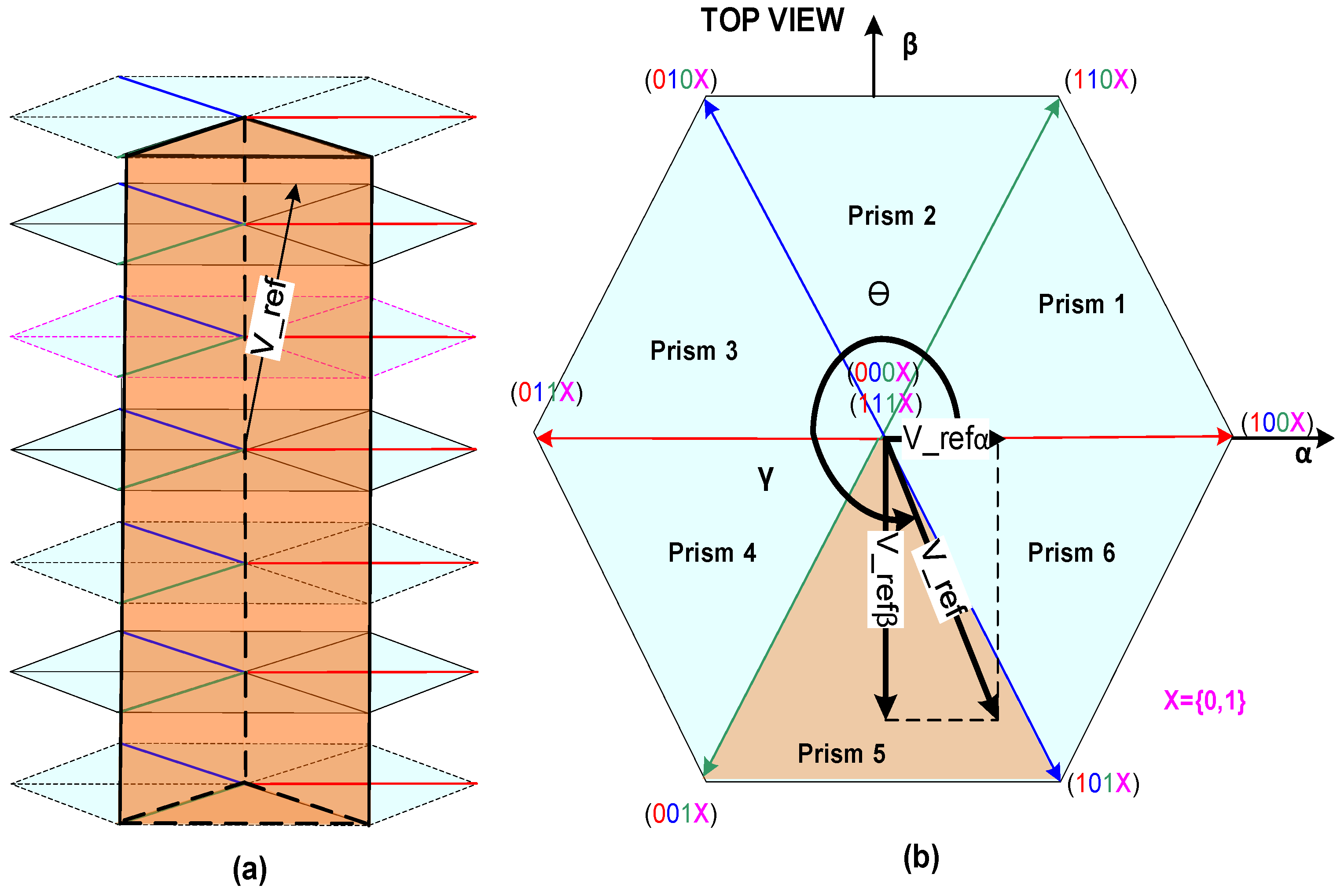
Figure 4.
Switching Space Vectors in α-β-γ frame: (a) 3D-View (b) Top View.
Figure 4.
Switching Space Vectors in α-β-γ frame: (a) 3D-View (b) Top View.
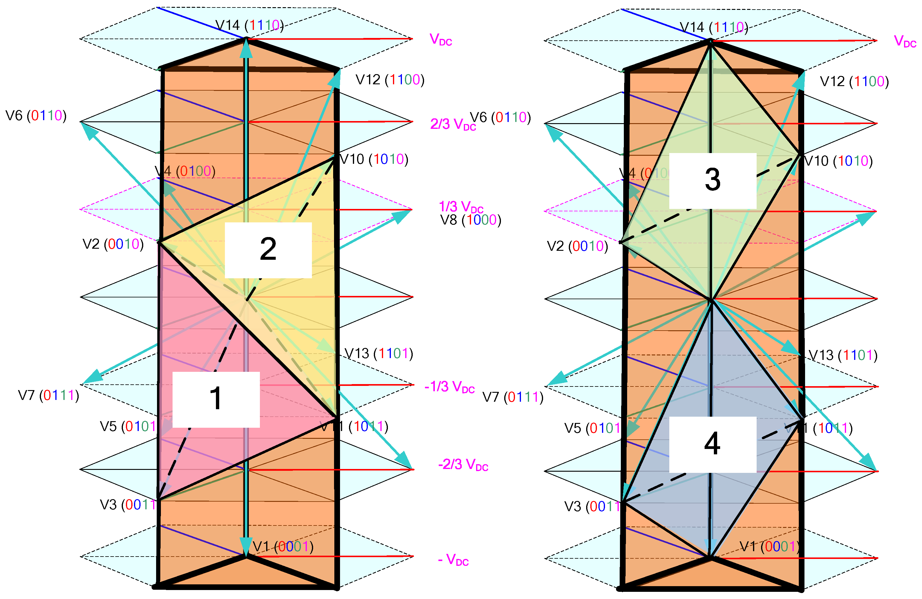
Figure 5.
Tetrahedron selection.
Figure 5.
Tetrahedron selection.
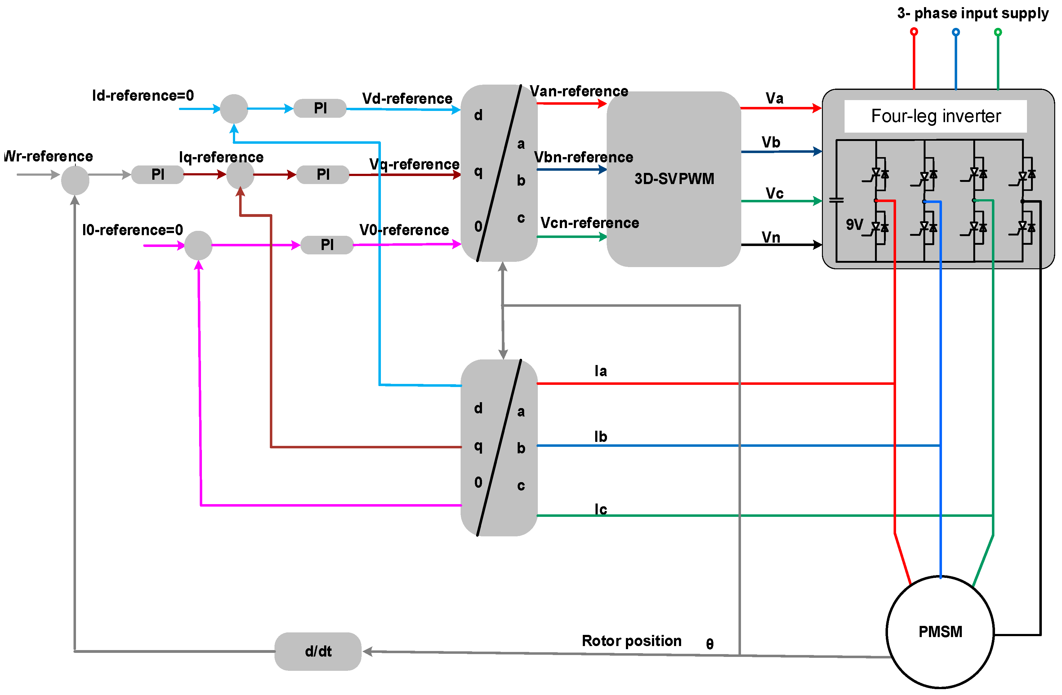
Figure 6.
Closed-loop field-oriented speed control topology using 3D-SVPWM for four-leg inverter proposed in [
25].
Figure 6.
Closed-loop field-oriented speed control topology using 3D-SVPWM for four-leg inverter proposed in [
25].
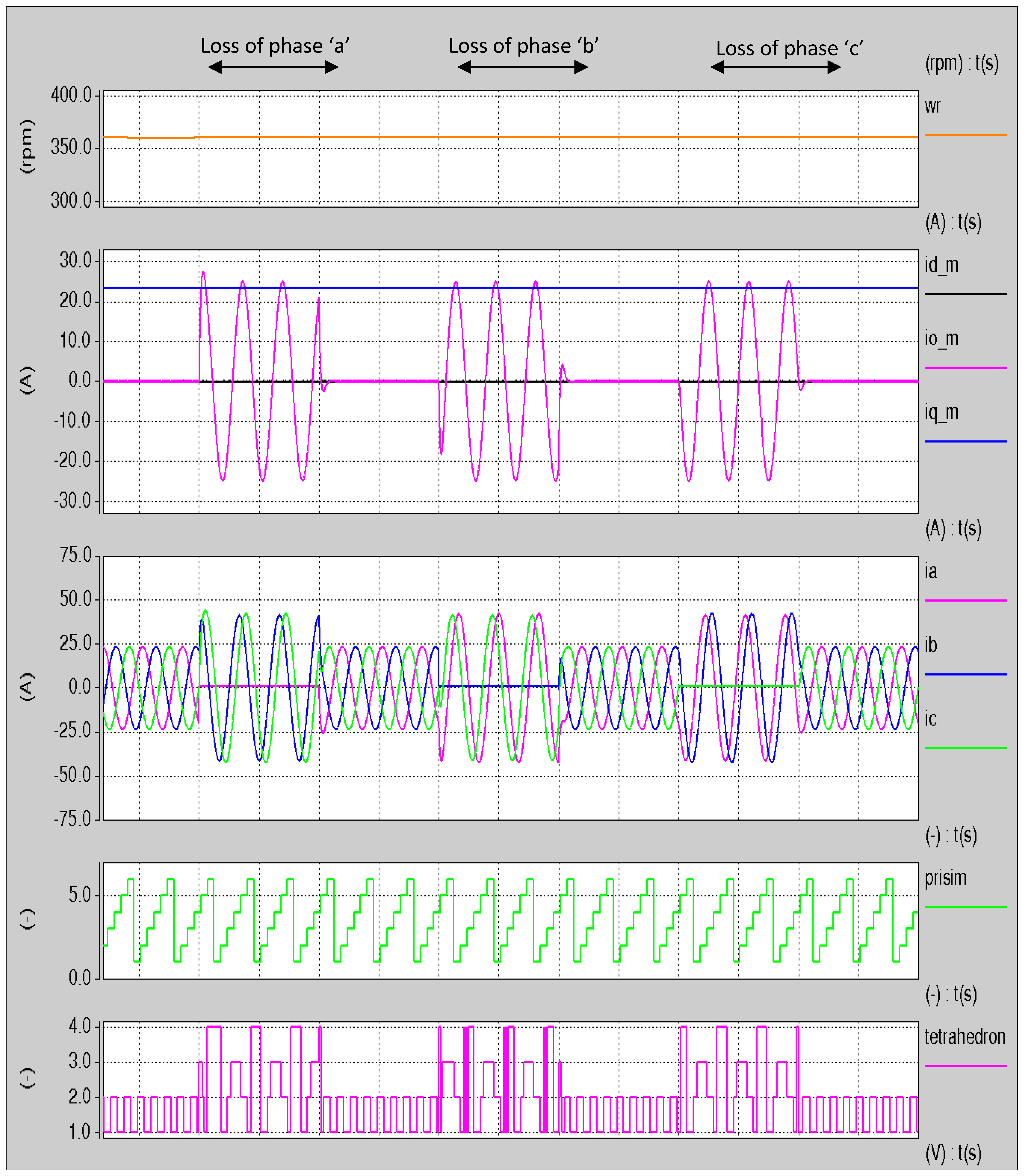
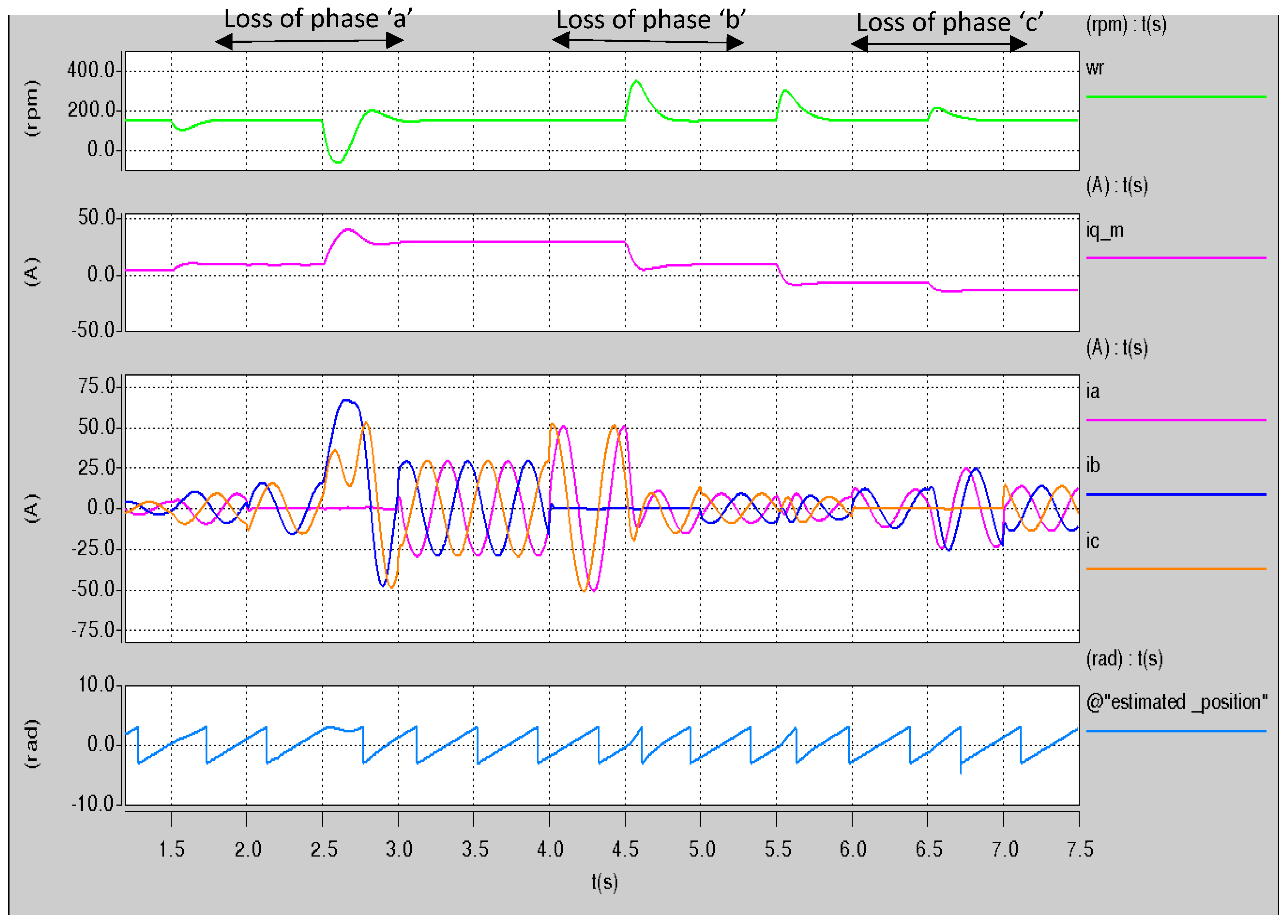
Figure 7.
Performance of the fault-tolerant PMSM drive system.
Figure 7.
Performance of the fault-tolerant PMSM drive system.
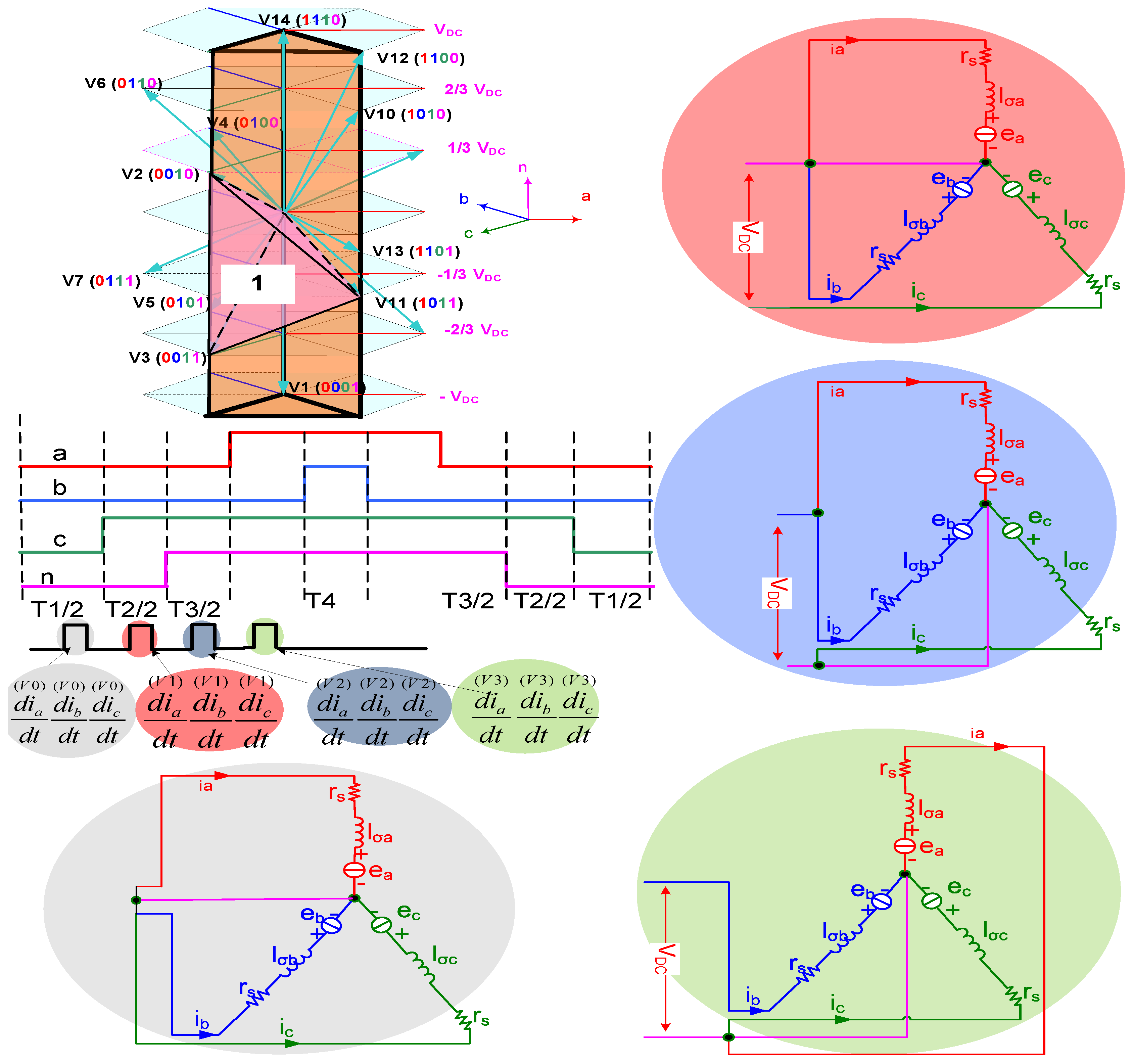
Figure 8.
Switching sequence for the case when the reference voltage exists in prism 5 and tetrahedron 1 in 3D SVM and the stator dynamic circuits under application of the voltage vectors V0, V1, V2, and V3 in normal operating conditions.
Figure 8.
Switching sequence for the case when the reference voltage exists in prism 5 and tetrahedron 1 in 3D SVM and the stator dynamic circuits under application of the voltage vectors V0, V1, V2, and V3 in normal operating conditions.
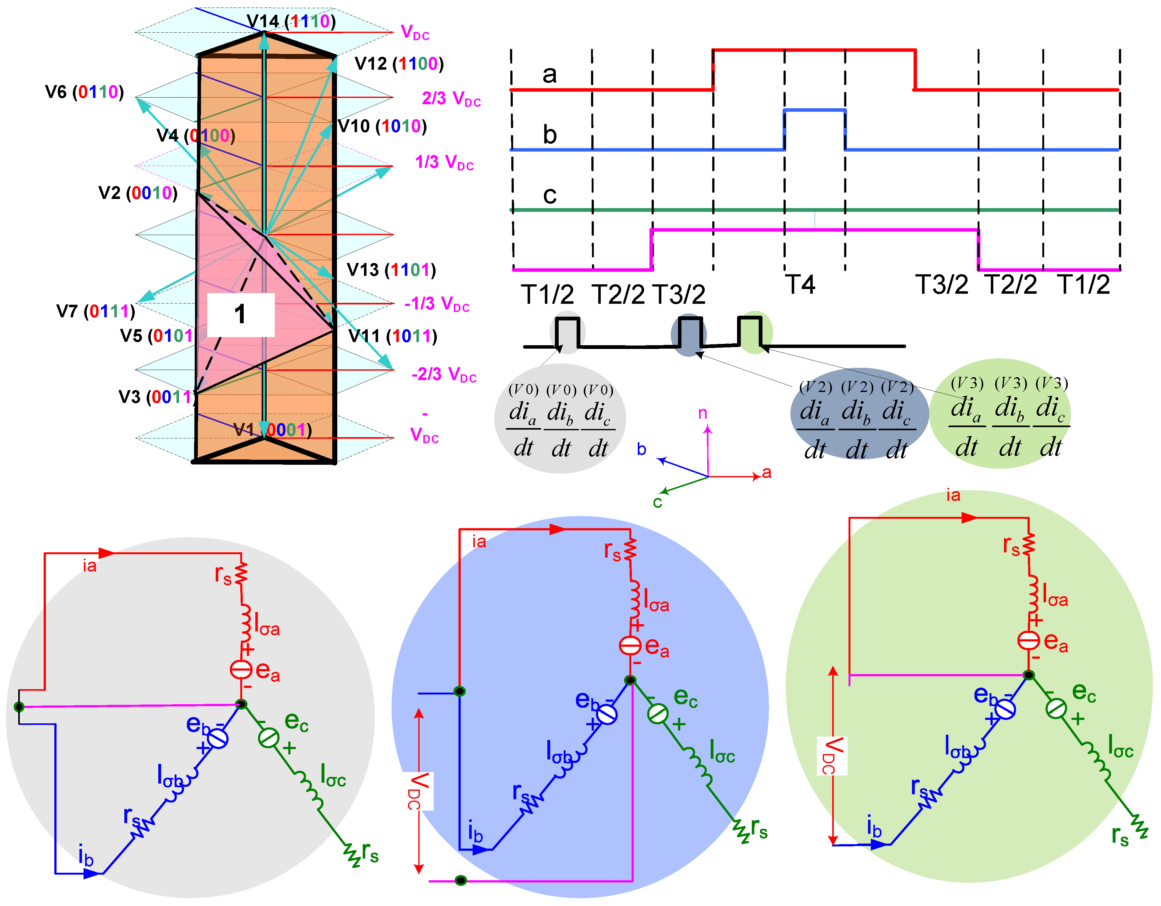
Figure 9.
Switching sequence in 3D SVM when the reference voltage exists in prism 5 and tetrahedron 1 and the stator dynamic circuits under application of the voltage vectors V0, V1, and V2 post a loss of phase “c”.
Figure 9.
Switching sequence in 3D SVM when the reference voltage exists in prism 5 and tetrahedron 1 and the stator dynamic circuits under application of the voltage vectors V0, V1, and V2 post a loss of phase “c”.
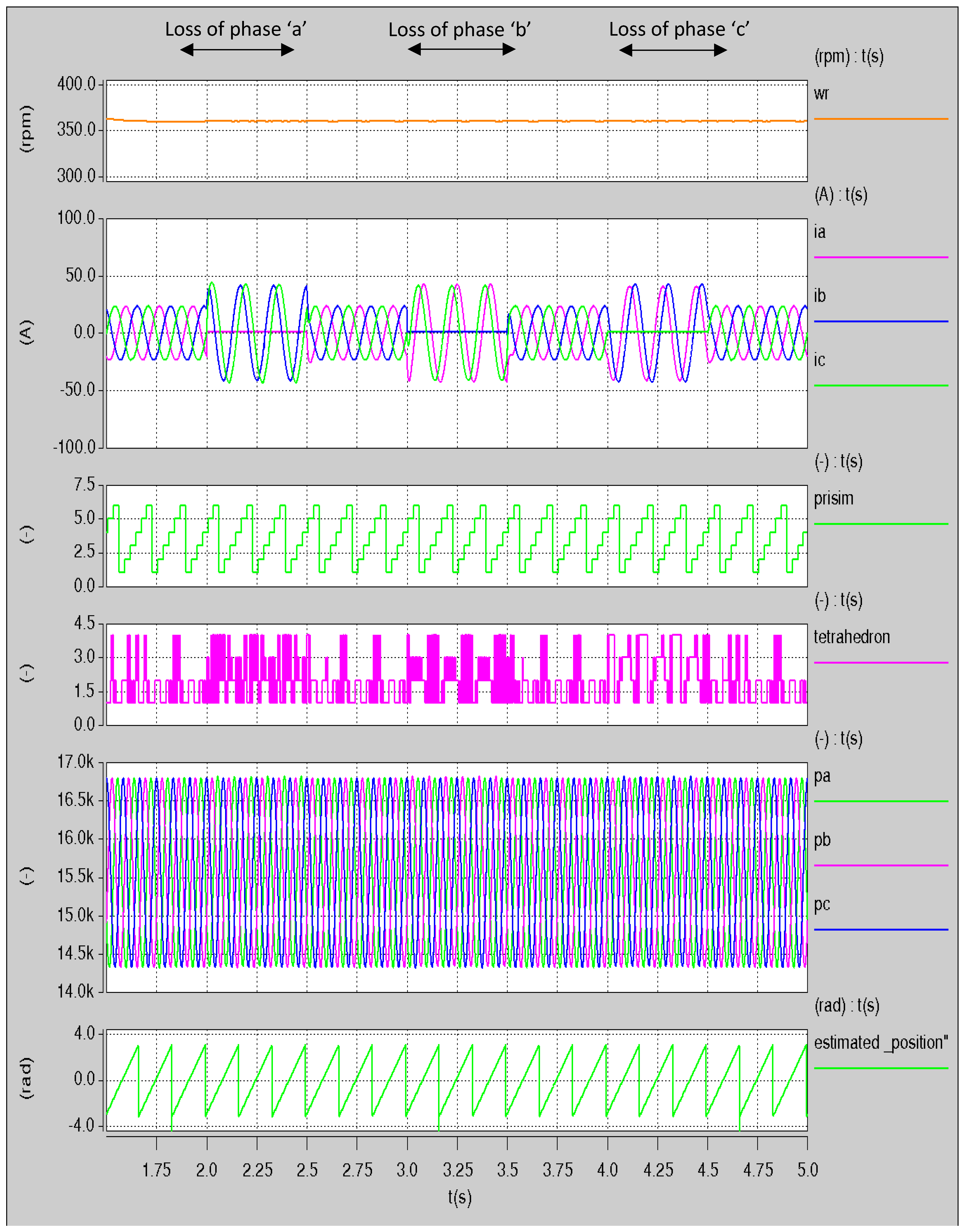
Figure 10.
Tracking the saliency in a 4-leg inverter using 3D-SVPWM under normal operating condition and post a loss of one phase.
Figure 10.
Tracking the saliency in a 4-leg inverter using 3D-SVPWM under normal operating condition and post a loss of one phase.
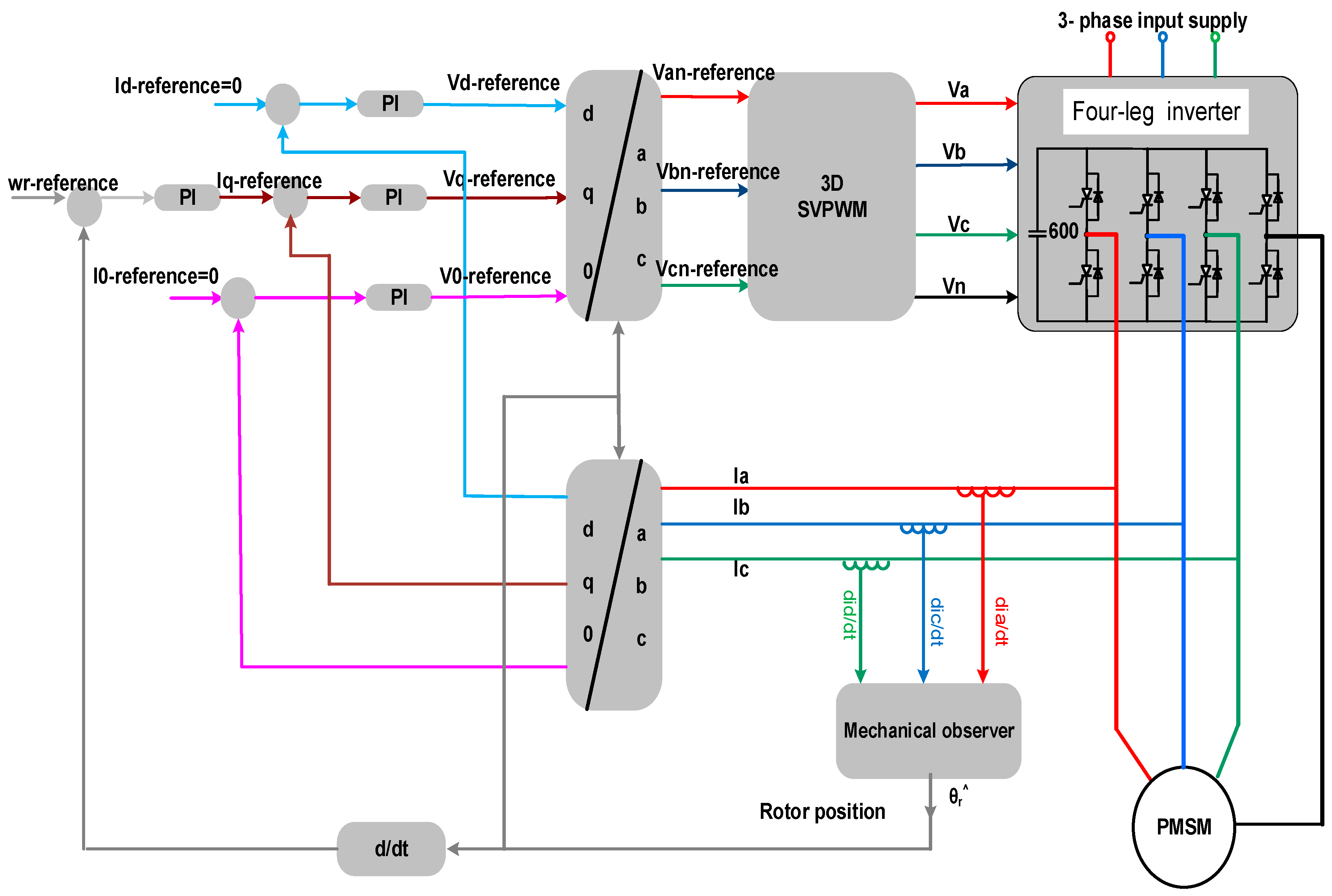
Figure 11.
Closed-loop field-oriented encoderless speed control topology using 3D-SVPWM under a loss of one phase.
Figure 11.
Closed-loop field-oriented encoderless speed control topology using 3D-SVPWM under a loss of one phase.
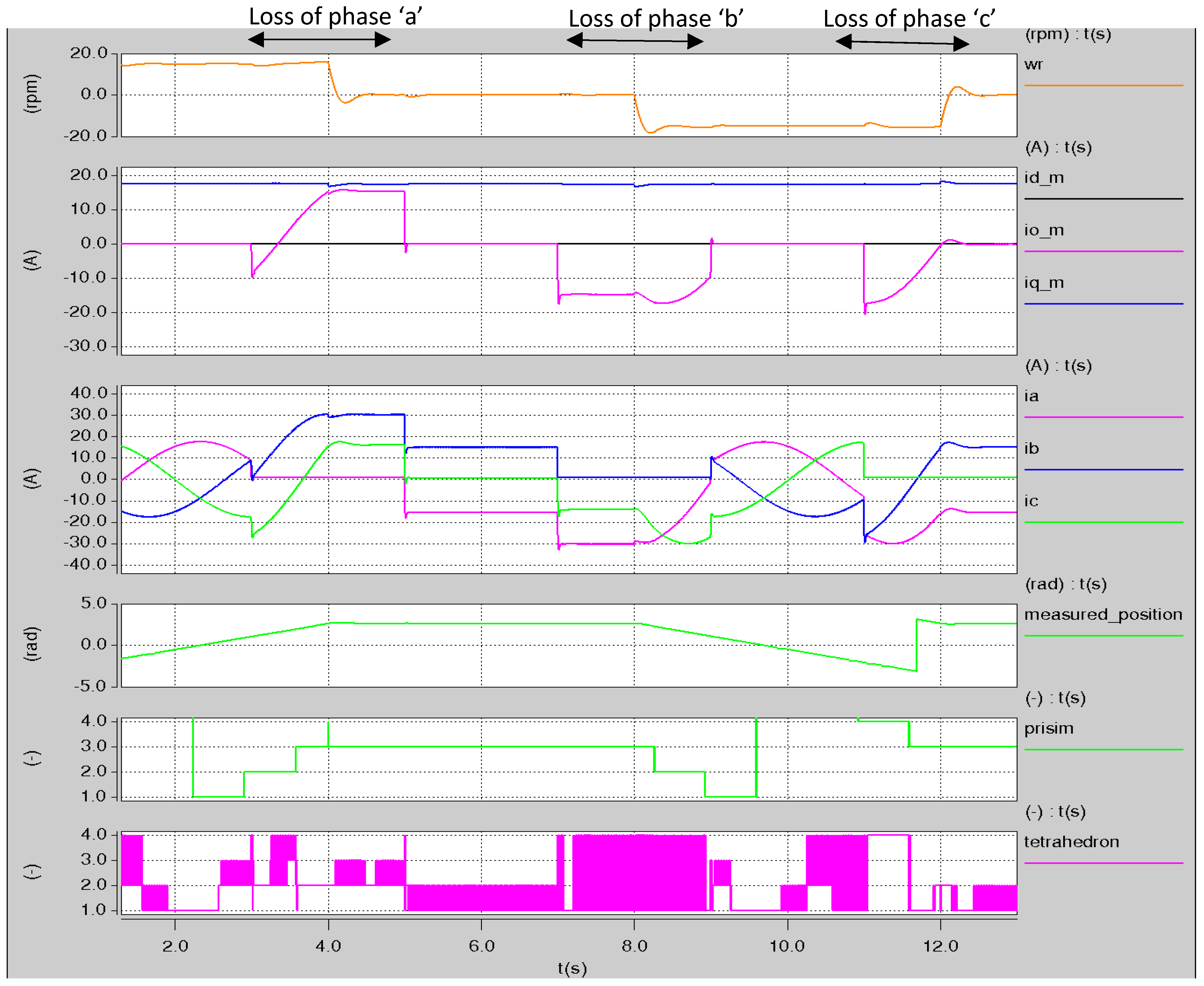
Figure 12.
Fully encoderless speed steps between –30 and 30 rpm under different operating conditions.
Figure 12.
Fully encoderless speed steps between –30 and 30 rpm under different operating conditions.
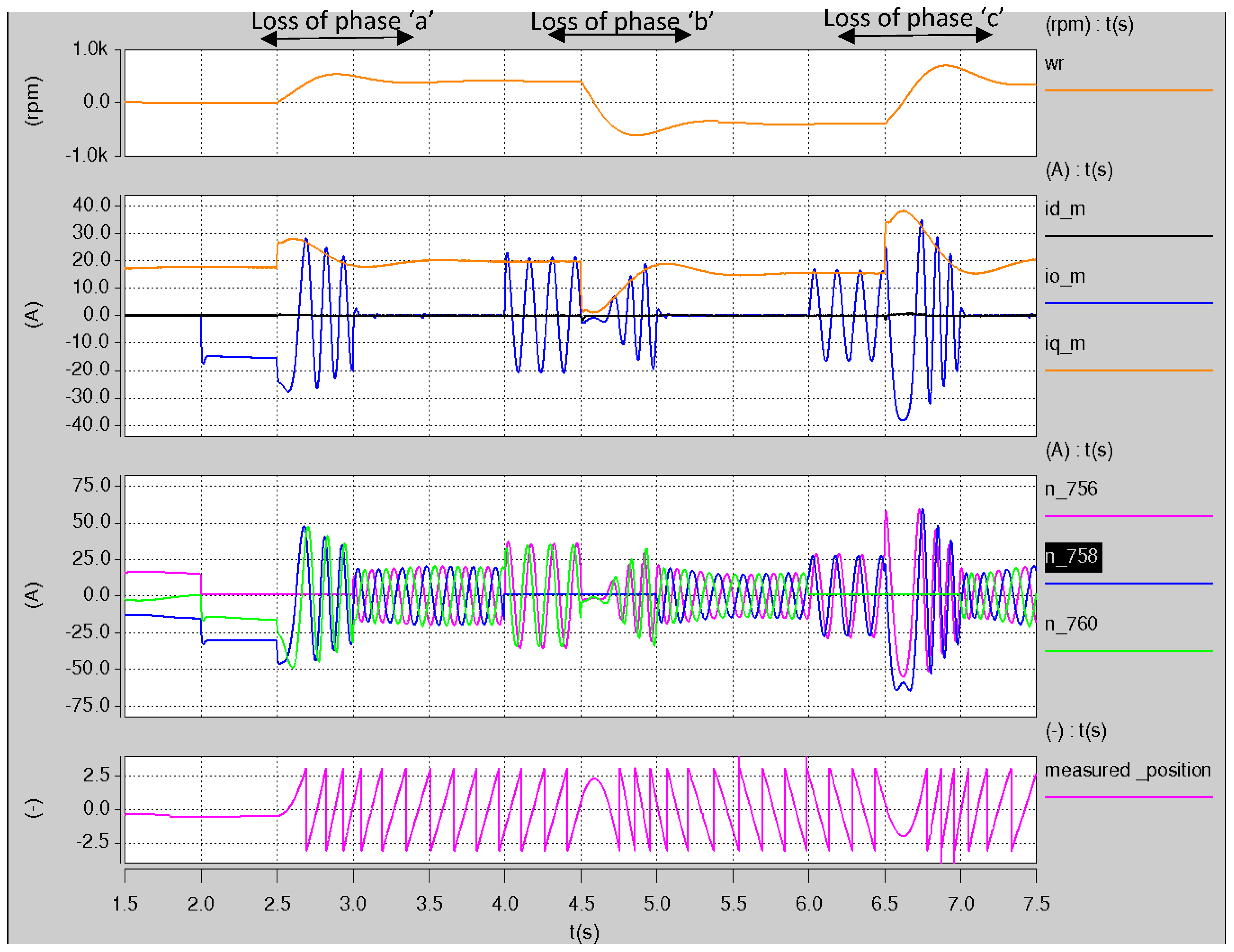
Figure 13.
Fully encoderless speed steps between 500 and −500 rpm under different operating conditions.
Figure 13.
Fully encoderless speed steps between 500 and −500 rpm under different operating conditions.
Figure 14.
Fully encoderless speed control under different load conditions.
Figure 14.
Fully encoderless speed control under different load conditions.
Table 1.
Selection of the prism.
Table 1.
Selection of the prism.
| Angle of Reference Voltage (θ) | Prism Number |
|---|
| 1 |
| 2 |
| 3 |
| 4 |
| 5 |
| 6 |
Table 2.
Selection of the tetrahedron.
Table 2.
Selection of the tetrahedron.
| Conditions | Tetrahedron |
|---|
| | | 1 |
| | | 2 |
| | | 3 |
| | | 4 |
Table 3.
Look up table for choosing correct switching sequence.
Table 3.
Look up table for choosing correct switching sequence.
| Prism | Tetrahedron | Switching Active Vectors |
|---|
| 1 | 1 | V8,V9,V13 |
| 2 | V8,V12,V13 |
| 3 | V8,V12,V14 |
| 4 | V1,V9,V13 |
| 2 | 1 | V4,V5,V13 |
| 2 | V4,V12,V13 |
| 3 | V4,V12,V14 |
| 4 | V1,V4,V13 |
| 3 | 1 | V4,V5,V7 |
| 2 | V4,V6,V7 |
| 3 | V4,V6,V14 |
| 4 | V1,V5,V7 |
| 4 | 1 | V2,V3,V7 |
| 2 | V2,V6,V7 |
| 3 | V2,V6,V14 |
| 4 | V1,V3,V7 |
| 5 | 1 | V2,V3,V11 |
| 2 | V2,V10,V11 |
| 3 | V2,V10,V14 |
| 4 | V1,V3,V11 |
| 6 | 1 | V8,V9,V11 |
| 2 | V8,V10,V11 |
| 3 | V8,V10,V14 |
| 4 | V1,V9,V11 |
Table 4.
Look up table for duty cycle computation.
Table 4.
Look up table for duty cycle computation.
| Prism | Tetrahedron 1 | Tetrahedron 2 | Tetrahedron 3 | Tetrahedron 3 |
|---|
| 1 | | | | |
| 2 | | | | |
| 3 | | | | |
| 4 | | | | |
| 5 | | | | |
| 6 | | | | |
Table 5.
Selection of the saturation saliency position scalars , , and for a fault-tolerant PMSM drive under normal operating condition.
Table 5.
Selection of the saturation saliency position scalars , , and for a fault-tolerant PMSM drive under normal operating condition.
| Prism | Tetrahedron 1 | Tetrahedron 2 | Tetrahedron 3 | Tetrahedron 4 |
|---|
| 1 | | | | |
| 2 | | | | |
| 3 | | | | |
| 4 | | | | |
| 5 | | | | |
| 6 | | | | |
Table 6.
Selection of the saturation saliency position scalars , , and for a fault-tolerant PMSM drive under a loss of phase “a”.
Table 6.
Selection of the saturation saliency position scalars , , and for a fault-tolerant PMSM drive under a loss of phase “a”.
| Prism | Tetrahedron 1 | Tetrahedron 2 | Tetrahedron 3 | Tetrahedron 4 |
|---|
| 1 | | | | |
| 2 | | | | |
| 3 | | | | |
| 4 | | | | |
| 5 | | | | |
| 6 | | | | |
Table 7.
Selection of the saturation saliency position scalars Pa, Pb, and Pc for a fault-tolerant PMSM drive under a loss of phase “b”.
Table 7.
Selection of the saturation saliency position scalars Pa, Pb, and Pc for a fault-tolerant PMSM drive under a loss of phase “b”.
| Prism | Tetrahedron 1 | Tetrahedron 2 | Tetrahedron 3 | Tetrahedron 4 |
|---|
| 1 | | | | |
| 2 | | | | |
| 3 | | | | |
| 4 | | | | |
| 5 | | | | |
| 6 | | | | |
Table 8.
Selection of the saturation saliency position scalars Pa, Pb, and Pc for a fault-tolerant PMSM drive under a loss of phase “c”.
Table 8.
Selection of the saturation saliency position scalars Pa, Pb, and Pc for a fault-tolerant PMSM drive under a loss of phase “c”.
| Prism | Tetrahedron 1 | Tetrahedron 2 | Tetrahedron 3 | Tetrahedron 4 |
|---|
| 1 | | | | |
| 2 | | | | |
| 3 | | | | |
| 4 | | | | |
| 5 | | | | |
| 6 | | | | |


