MDEAN: Multi-View Disparity Estimation with an Asymmetric Network

Abstract

In recent years, disparity estimation of a scene based on deep learning methods has been extensively studied and significant progress has been made. In contrast, a traditional image disparity estimation method requires considerable resources and consumes much time in processes such as stereo matching and 3D reconstruction. At present, most deep learning based disparity estimation methods focus on estimating disparity based on monocular images. Motivated by the results of traditional methods that multi-view methods are more accurate than monocular methods, especially for scenes that are textureless and have thin structures, in this paper, we present MDEAN, a new deep convolutional neural network to estimate disparity using multi-view images with an asymmetric encoder–decoder network structure. First, our method takes an arbitrary number of multi-view images as input. Next, we use these images to produce a set of plane-sweep cost volumes, which are combined to compute a high quality disparity map using an end-to-end asymmetric network. The results show that our method performs better than state-of-the-art methods, in particular, for outdoor scenes with the sky, flat surfaces and buildings.

1. Introduction

Disparity estimation from images is playing an increasingly important role in computer vision. Numerous important applications, including 3D reconstruction, autonomous driving, robotics and medical image processing, require depth information (disparity and depth can be converted to each other under certain circumstances). Thanks to multi-view based methods, depth can be computed with high precision.

Conventional multi-view depth estimation methods, such as Structure-from-Motion (SFM) algorithms [1], are effective 3D reconstruction algorithms, which use a sequence of two-dimensional images containing motion information to estimate the three-dimensional structure of a scene using triangulation [2]. Besides SFM, there are many conventional Multi-View Stereo (MVS) methods to estimate the depth map by computing the cost volume using the plane-sweep method [3] or by measuring the similarity between patches using some error functions [4]. There are other methods which combine shading or other information with stereo to capture the 3D scene information; for instance, Langguth et al. [5] propose a method which combines stereo and shape-from-shading into a single optimization scheme for multi-view reconstruction. Kim et al. [6] propose using multiple stereo pairs of spherical images to reconstruct a block-based scene. Haene et al. [7] integrate semantic information with 3D reconstruction. These methods have used different constraints with MVS to improve the reconstruction accuracy. While conventional MVS methods have many advantages, some of the operations incur additional overhead in computing resource and hence, require more time, e.g., parallel distributed matching [8] or methods that incorporate geometric constraints [9].

Deep convolutional neural networks (CNNs) have achieved great success in image classification [10] and in semantic segmentation [11]. Yin et al. [12] present an unsupervised multilevel segmentation scheme for automatically segmenting grayscale and color images. Recently, CNNs have been used to learn the relationship between color pixels and depth information in a single image [13]. In previous work with deep learning based stereo, CNNs are generally used to learn the similarity of patches for stereo matching [14]. Compared with traditional methods, there are many advantages of deep learning based methods. For example, a CNN-based method does not need to rely on handcrafted features. Moreover, it does not have to do explicit feature matching. However, current deep learning based methods still have limitations. For example, the positions, poses of the cameras and the number of input images are limited. Therefore, the motivation of our model is to address these limitations and to improve the accuracy of current deep learning based methods.

In this paper, we present a new CNN-based method called MDEAN which stands for a multi-view disparity estimation method using an asymmetric network. The network is inspired by the work of Huang et al. [15] and Mayer et al. [16]. First, a reference image and an arbitrary number of adjacent images are selected. Second, the pose of each camera is computed using the standard SFM scene reconstruction algorithm [1]. Next, for each adjacent image, a cost volume is computed using the plane-sweep method [4] as input to the network. Then, an asymmetric encoder–decoder network with skip connections and disparity estimation layers is used to estimate the disparity information of the scene. Finally, max pooling is used to aggregate the disparity information extracted from each patch, and convolution is used for the final disparity prediction. Based on the experimental results, our proposed method can obtain high-quality disparity maps (See Figure 1). Moreover, it outperforms the state-of-the-art methods with better prediction results, in particular, in outdoor scenes with the sky, flat surfaces, buildings.

2. Related Work

Disparity estimation is of significant importance to the field of computer vision research and has been widely studied. Early image-based disparity estimation commonly uses multi-view based SFM and MVS methods [17]. Recently, depth estimation using deep learning has become popular in computer vision [18]. Deep learning based depth estimation has been widely used in monocular images [19]. However, unlike multi-view images, monocular images cannot capture sufficient information in the scene. Thus, the accuracy of single view depth estimation is not comparable to that of multi-view methods. In this paper, we focus mainly on multi-view disparity estimation.

2.1. Monocular Depth Estimation

Depth estimation for monocular images before the advent of learning based methods commonly uses MRF [20] and CRF [21]. Recent significant advances in machine learning and deep learning have motivated recent research in using deep learning for depth estimation [13]. The vast majority of deep learning based depth estimation methods are applied to monocular image depth estimation. One of the earliest methods proposed by Eigen et al. [18] uses a multi-scale neural network to predict depth. Before the introduction of Fully Convolutional Networks (FCN) [11], many deep learning based methods estimate the depth map at the global level with a fully connected network at the last level. Recently, many depth estimation methods are trained end-to-end based on the FCN network structure, which can handle images of any size. Laina et al. [13] propose a depth estimation method using a deeper residual network. Godard et al. [19] attempt to estimate depth by incorporating the left-right consistency constraint. Mancini et al. [22] use a fully convolutional architecture combined with LSTM for depth estimation. Li et al. [23] propose a deep end-to-end learning framework to estimate depth using a single image and Zhang et al. [24] use a novel deep Hierarchical Guidance and Regularization (HGR) learning framework for end-to-end monocular depth estimation. The network structures of the above methods are all FCN, and all of them have achieved encouraging results. Our network is also based on the FCN network structure and has incorporated important novel improvements.

2.2. Multi-View Depth Estimation

Before the advent of deep learning, disparity estimation of images is mostly realized by SFM and MVS methods. Conventional SFM is a method of reconstructing the scene structure by the motion of a camera or a sequence of unordered images. The core algorithm selects a set of appropriate images for determining the camera’s parameters. Conventional MVS methods estimate the 3D information by multiple images of known camera positions, and can be classified and evaluated according to several criteria. Recently, many MVS 3D reconstruction systems have been proposed, e.g., PMVS [25], CMVS [26] and COLMAP [17]. All of them can produce excellent reconstruction results. In particular, Schonberger et al. present the COLMAP system which uses photometric and geometric priors to select pixel-level views. COLMAP performs best in multi-view stereo [17]. In our work, we use the parameters and poses of the cameras estimated by COLMAP as part of our input to estimate more accurate disparity maps.

Deep learning is an important method in reconstructing a scene in 3D and in obtaining other scene information. Some methods estimate the disparity map by learning patch matching or by learning to find correspondences between patches [15] in multi-view images, while other methods use the plane-sweep volume as input to generate the disparity image [27]. Many multi-view based depth estimation methods such as Sunghoon et al. [3] use the method of dense depth reconstruction based on geometry. The cost volume is learned using 3D convolutions of concatenated warped and reference features. The cost volume is adjusted based on a context aware aggregation cost, and the dense depth map is regressed from the cost volume. Huang et al. [15] use camera parameters to select a reference image and a set of neighboring images to compute the plane sweep volume. The reference image features are extracted by the encoder of the pre-trained VGG-19 network, then the plane-sweep volume patch matching results and VGG features are used as the input to the intra-volume feature aggregation network for depth estimation. Pizzoli et al. [28] propose a method combining bayesian estimation and convex optimization, which can accurately predict in real time the scene depth of each pixel of an image sequence. Yao et al. [29] use differentiable homography warping to construct the cost volume, and then refine an initial depth map with the reference image feature to generate the final output. Their method is based on an MVSNet structure, which is a four-layer U-Net. In contrast, we propose a new asymmetric model to estimate the depth information. Ummenhofer et al. [30] take two images as input and estimate the depth and motion, but their method is designed to handle only two views. Our proposed MDEAN can handle any number of views. Similar to depth estimation discussed above, there is much progress in depth estimation based on optical flow computation in recent years. For example, Deqing et al. [31] propose using optical flow estimation to distort CNN features to construct the cost volume, from which the depth is estimated. Shi et al. [32] propose a method which does not need any prior information of the parallax range. From two warping error measures, an accurate estimate can be made in occluded regions and contours. Jiang et al. [33] propose a method to estimate disparity by fine-tuning FlowNet2.0 network, and the coarse estimates are fused, and refined by a multi-view stereo refinement network. However, many of the above methods share many constraints. For example, the number of input images is fixed [30], and the input image size is fixed [28] as well. In this paper, our proposed method for disparity estimation can take an arbitrary number of images and the images can be of arbitrary size.

2.3. Depth Estimation

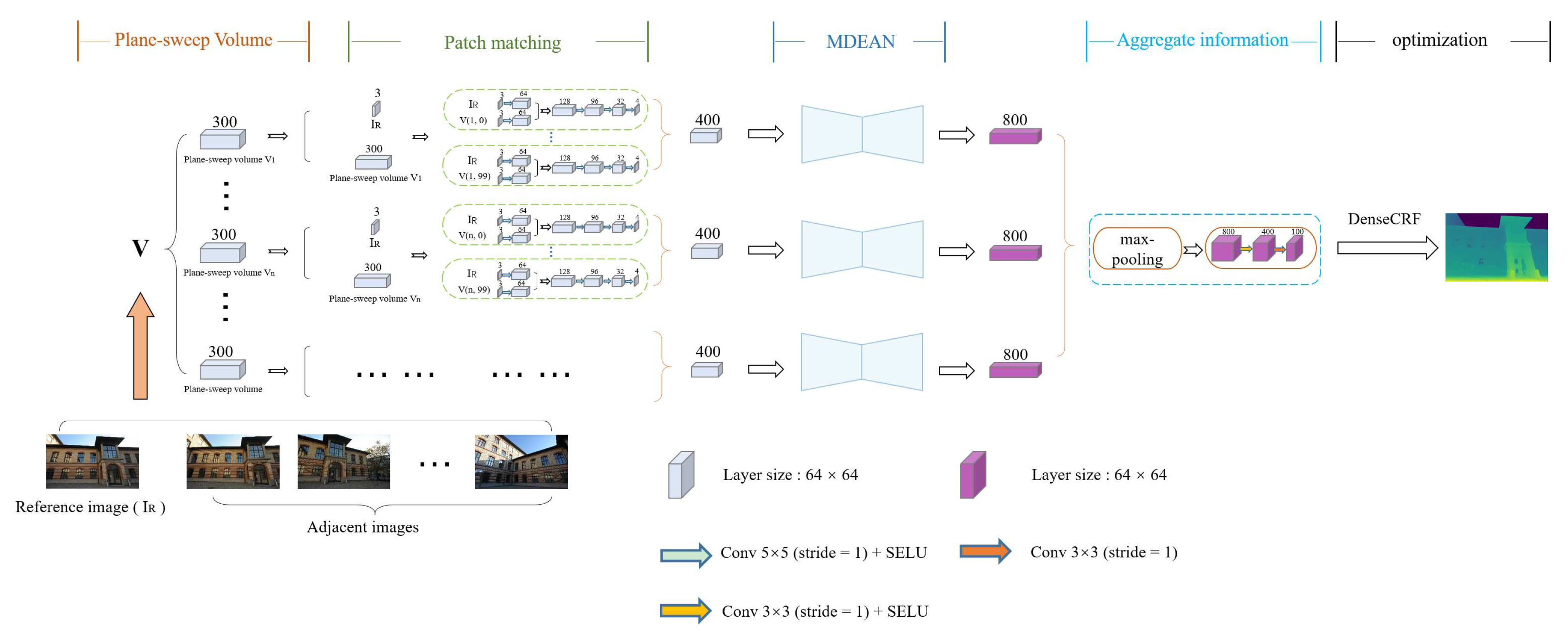
Our proposed method to estimate disparity map of multi-view images is a fully convolutional network based on the encoder–decoder architecture. It takes a set of plane-sweep volumes as input and produces high-quality disparity maps. In order to correctly estimate the disparity of the sky, specular objects, thin structures and scenes that may even have errors in the ground truth data, the training set includes real scenes and synthetic data (Section 4.1). Training with two types of datasets are used to achieve more accurate estimation results. The experimental results show that our method is more accurate than other state-of-the-art methods in both qualitative and quantitative evaluation (Section 4).

3. MDEAN

A novel asymmetric network which uses multi-view for disparity estimation is described in this section. First, an introduction of how to construct the input for our network is given. Then, the asymmetric network structure is introduced. Finally, relevant optimizations for generating the disparity maps are explained.

3.1. Problem Definition

We estimate the disparity map of a scene using a set of images, camera poses and corresponding calibration results. Denote I = {$I_k$∣k = 1, 2, …, N} as the set of input images. The set of poses of cameras is denoted as P = {$P_k$∣k = 1, 2, …, N}. The disparity map is represented by D. We select an image as the reference image $I_R$, R ∈ {1, 2, …, N} in I, and other images {$I_k$∣k ∈ {1, 2, …, N} ∩ k ≠ R} are denoted as adjacent images. The goal is to use the adjacent images and the reference image (Section 3.2) to estimate the disparity map.

3.2. Network Input

We first use COLMAP to perform sparse reconstruction using the set of input images to compute the poses of the cameras and the camera calibration parameters. Next, the plane-sweep volume for each adjacent image is computed. Then, all the plane-sweep volumes of all adjacent images are input to the proposed MDEAN.

For calculating the plane-sweep volume, we set a disparity parameter $\mathsf{\Theta }$ and a disparity level $\widehat{D}$ of the scene. The disparity level, 0 × $\mathsf{\Theta }$ denotes the minimum disparity, and $(\widehat{D}-1)$ × $\mathsf{\Theta }$ denotes the maximum disparity. The parameter $\mathsf{\Theta }$ changes with the disparity level. The more the disparity levels, the smaller is the $\mathsf{\Theta }$ and vice versa. For each disparity level, an adjacent image is warped to the reference image to form a layer in the volume. In principle, the warped image closely aligns with the reference image. After finishing the above steps for all the adjacent images, the plane-sweep volume can be calculated. We define the plane-sweep volume as V = {$V_{n,d}$ ∣ n ∈ {1, 2, …, N} ∩ n ≠ R, d ∈ {0, 1, …, $\widehat{D}-$ 1}}, $V_{n,d}$ represents a single patch of the nth adjacent image and the dth disparity layer (See Figure 2). During training, we set the maximum number of levels of disparity to 100 to prevent the GPU memory to overflow.

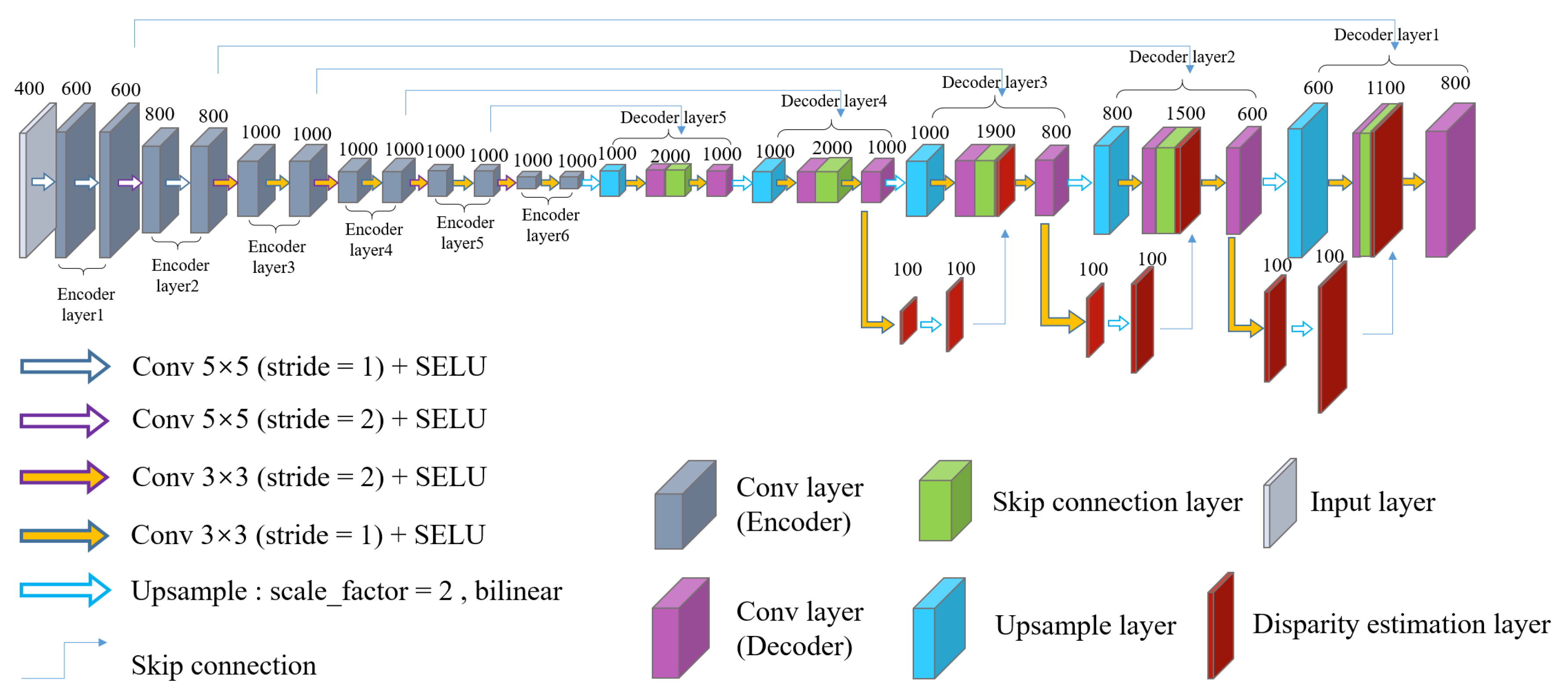
3.3. Architecture of MDEAN

We propose an asymmetric fully convolutional network based on the encoder–decoder structure for scene disparity estimation. The structure of MDEAN is shown in Figure 3. The fully convolutional neural network is first proposed by Long et al. [11], which can easily adapt to an end-to-end framework without restriction of image size. The encoder–decoder structure includes an upsampling operation using transpose convolution, and is extended with skip connections from the encoder to the decoder layer by Ronneberger et al. [34]. Therefore, the number of decoders is equal to the number of encoders. We propose a new asymmetric fully convolutional structure based on the encoder and decoder structure which can extract better feature information of an image. In the encoding layer, more and more detailed feature information can be extracted and transferred to the decoding layer. At the same time, the scale of space volume obtained by each decoding layer is doubled, and scene information can be restored with more detailed features. Thus, the proposed MDEAN can better estimate the disparity of the image.

Traditional methods commonly find corresponding pixels of two adjacent frames using handcrafted features and optimize some image-based error functions. In the proposed method, we use convolution for patch matching operations. In particular, we perform convolution operation using a patch extracted from reference image $I_R$ and from $V_{n,d}$. Because the maximum number of levels of disparity is 100, we perform 100 sets of convolution operations for each adjacent image. After each set of convolutions, a volume with four channels is generated. Finally, the 100 sets of volumes are stacked to generate a new volume with 400 channels, which is input to the MDEAN for disparity prediction. The details of the network structure are shown in Figure 4.

We use these 400-channel patch matching features as input to our proposed MDEAN, which is based on DispNet [16]. However, we make some important refinements to make the estimation more accurate. Our network contains an asymmetric structure which consists of six encoders and five decoders. Symmetric network structures have also been tried in the experiment, such as the five-encoder and five-decoder structure, and the six-encoder and six-decoder structure, but their results are not as good as the proposed structure. In Section 4.5, our evaluation shows that the proposed asymmetric network is better than symmetric networks with more accurate disparity estimation. The first five encoders are skip connected to the five decoders, which can resolve detailed features. We also import three disparity estimation layers [19] to the decoder to add the spatial resolution of subsequent scales. The activation function layers used in our network are all Scaled Exponential Linear Unit (SELU) layers proposed by Klambauer et al. [35], which have self-normalizing property that makes our network more robust. Our network uses many convolutional kernels throughout the encoders and decoders to enhance the ability of extracting detailed features. In a typical encoder–decoder architecture, the number of encoders is equal to the number of decoders, so that the output image size can be the same as that of the size of the input image. In the proposed architecture, however, up-sampling is used before the convolution in the fifth layer of the decoder. Thus, MDEAN can use an asymmetric structure of encoder–decoder while maintaining compatible size between the input and the output.

In the last part of the network structure, inspired by PointNet [36], we use element-wise max-pooling to aggregate information from any number of patch volumes, and to ensure that the aggregated results are in the same order as that of the adjacent images. Then, the features are extracted by the convolutional layers to generate the final disparity map.

We use the cross entropy loss function (Equation (1)) to train our network, because we consider image disparity estimation as a multi-class classification problem, in particular,

$$L(q,i)=-log\frac{exp\left(q_i\right)}{{\sum }_{j=1}^{C}exp\left(q_j\right)}$$

(1)

where $q_i$ denotes the probability of the target class i and $q_j$ denotes the probability of the $j$th class and i, j ∈ {1, 2, …, C}, C denotes the number of classes.

The pseudocode of the proposed algorithm is presented in Algorithm 1.

In order to refine our final prediction results, we apply the initial prediction to the Fully-Connected Conditional Random Field (DenseCRF) [37].

Algorithm 1 Disparity estimation algorithm based on an asymmetric structure.

Use COLMAP [17] to generate camera internal parameters and poses using an image sequence;  Construct plane-sweep volumes of adjacent images and the reference image;  Input the reference image, plane-sweep volumes of adjacent images, and ground truth disparity  maps of the reference image to the network;  while iterations t < $T_{train}$ do   for each minibatch(=1) from the training set do    for each adjacent volume of the reference image do     for each layer in the volume do      Each layer is convolved with the reference image to generate a 4-channel volume shown in Figure 4;     end for     Stack all generated volumes;     Disparity estimation is carried out by the MDEAN shown in Figure 3 and generate a volume containing disparity;    end for    Aggregate information from any number of volumes using max-pooling operation and extract    features by convolution to generate the disparity map;    Calculate the loss according to Equation (1) and the ground truth disparity maps, and perform    back propagation to update each weight w in the network.   end for  end while

4. Results

4.1. Dataset

We use the DeMoN dataset [30] and the MVS-SYNTH dataset [15] to train our network. In the DeMoN dataset, a real-world scene dataset and a synthesized dataset are included. However, the ground truth for the real-world dataset may include errors of measurement during the acquisition process, in particular, in areas such as the sky, areas with specular reflection, and in thin structures. The synthesized data is not realistic enough to accurately reflect the appearance of the real world. Thus, we also include MVS-SYNTH in the training set, a synthetic dataset with better shadow effect that resembles the real world better.

To evaluate our method, we use the high-resolution multi-view dataset ETH3D [38], which consists of 13 scenes, and includes both indoor and outdoor scenes. ETH3D also provides laser scanned point clouds for corresponding scenes, and the laser scanned of each point cloud is projected onto the image of each view to obtain the corresponding ground truth disparity map. We use it to evaluate the efficacy of our approach on real scenes. In addition to using the ETH3D dataset, we also capture some outdoor scenes to verify the robustness of our algorithm.

4.2. Experimental Details

Our training process is divided into two steps. First, we replace the MDEAN with two simple $3\times 3$ convolution layers for pre-training. Next, we replace the two convolution layers with MDEAN and use the pre-trained network parameters for subsequent training.

The COLMAP system [17] is used to estimate the cameras’ internal parameters, external parameters and image poses. These parameters are used to generate the cost volume as input to the network.

We use $64\times 64$ patches as input to the MDEAN. Thus, the network can be stored easily in the GPU memory during training. Using the input image patches, an encoder layer generates the feature vector, which is passed to the corresponding decoder layer for pixel wise disparity estimation. The network output is also $64\times 64$ patches. We then tile these patches to generate the complete disparity map.

For both training stages, pre-training and training, we used Adam [39] and set the learning rates of ${10}^{-5}$ and ${10}^{-6}$, respectively, for the two stages to achieve better results. We also utilize L2-norm of the gradients at each layer to constrain the training process and use gradient clipping to prevent gradient explosion.

In our implementation, the network structure is implemented in PyTorch in a system with an NVIDIA TITAN Xp graphics card. Both pre-training and training take nearly two days.

4.3. Evaluation Method

Three different geometric methods including geometric errors [15], L1-rel [30] and SC-inv [18] are utilized to evaluate the performance of our method and of the state-of-the-art methods.

The geometric error L1-inv is obtained by calculating the L1 distance between the ground truth and the estimated disparity map and ignoring pixels without ground truth information. Its expression is defined as:

$$L1-inv=\frac{1}{m}\sum _i\left|\frac{1}{d_i}-\frac{1}{{\widehat{d}}_i}\right|$$

(2)

L1-rel is the relative error defined as:

$$L1-rel=\frac{1}{m}\sum _i\frac{|d_i-{\widehat{d}}_i|}{{\widehat{d}}_i}$$

(3)

where $d_i$ denotes the estimated depth value and ${\widehat{d}}_i$ the ground truth value. m denotes the number of valid pixels.

SC-inv uses a scale-invariant error to measure the relationship between two values. The expression is defined as:

$$SC-inv=\sqrt{\frac{1}{m}\sum _i{z_i}^2-\frac{1}{m^2}{\left(\sum _i{z}_i\right)}^2}$$

(4)

where $z_i=log{d}_i-log{\widehat{d}}_i$.

In order to more intuitively reflect the advantages and disadvantages of different methods. We utilize the range transformation method Equation (5) and the z-score standardization method Equation (6) to normalize the values obtained by the above three geometric measures, and

$$x_m=\frac{x_i-min\left(x\right)}{max\left(x\right)-min\left(x\right)},$$

(5)

$$x_n=\frac{x_i-mean\left(x\right)}{\sigma },$$

(6)

where $x_i$ denotes a number that needs to be normalized, x the set of numbers, and $\sigma$ the standard deviation of all the numbers that are normalized. $x_m$ denotes the result of the range transformation method and $x_n$ the result of the z-score standardization method.

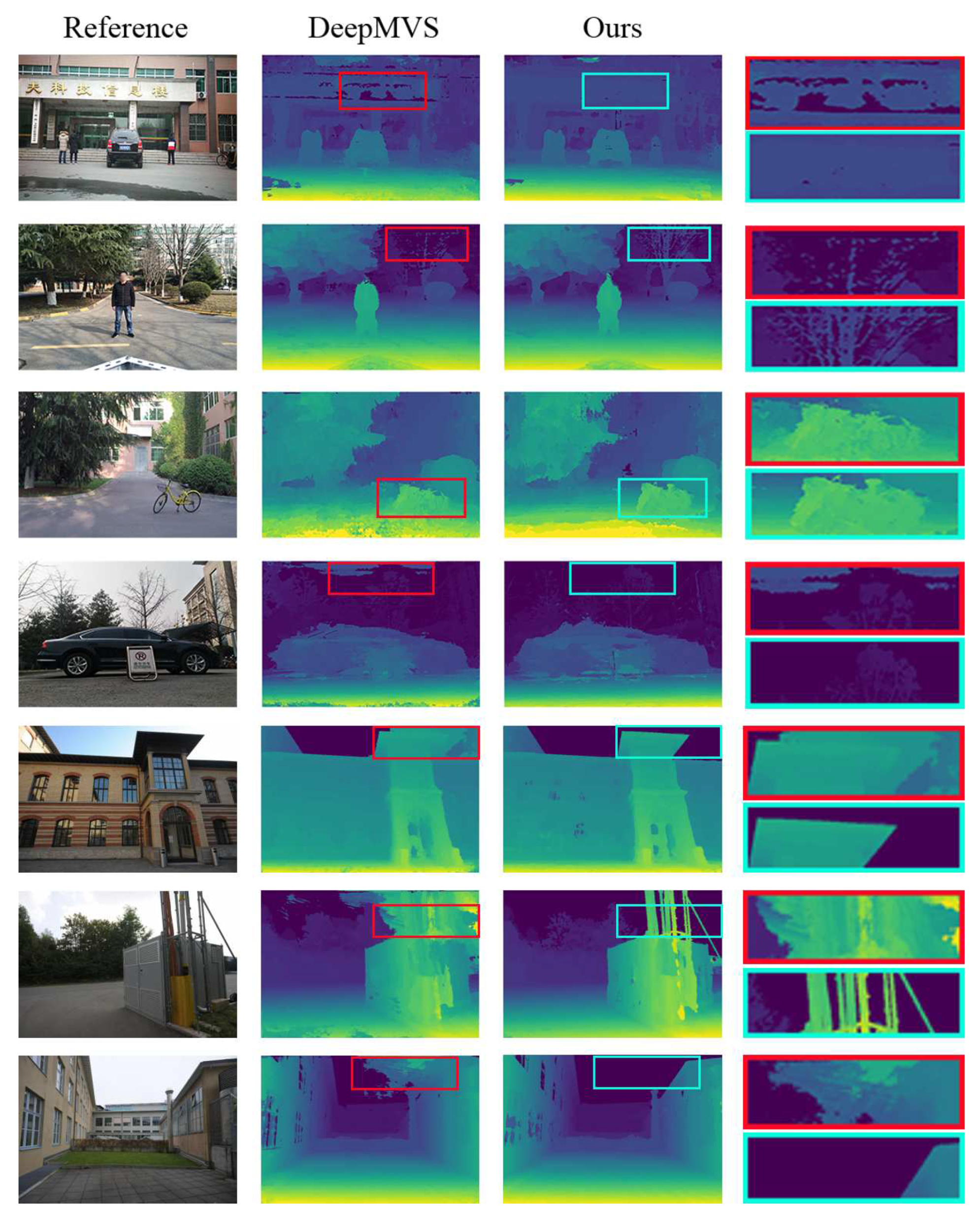
4.4. Evaluation Results

Among traditional algorithms such as PMVS [25], MVE [40] and COLMAP [17], we choose COLMAP to compare with our method, because compared with the other two traditional methods, the COLMAP results are the best on the ETH3D dataset. If not explicitly stated, we use the default settings of COLMAP. An option to filter out geometric inconsistencies is provided in COLMAP. In any case, the filtered disparity map may reduce the impact of the method on the results. Thus, we compare the results without filtering.

We also compare our results with the results of DeMoN [30]. It should be noted that DeMoN can be used for disparity estimation of image pairs only. Therefore, we extend DeMoN to multi-view disparity estimation. The extended method aggregates information from all available image pairs using the median of corresponding pixels in the final disparity map. Since DeMoN uses a fixed image size for disparity estimation, we crop the images in ETH3D to the appropriate size and then use DeMoN for estimation. In the experiments, we select the central parts of the ETH3D images for estimation.

DeepMVS is a multi-view disparity estimation convolutional neural network algorithm [15]. It generates a set of scan volumes by inputting any number of images, and then estimates the corresponding disparity map using the convolutional neural network. In addition to comparing with DeepMVS and DeMoN, we also compare our results with that of the latest methods DPSNet [3] and MVSNet [29]. These two methods have very good performance in multi-view stereo reconstruction.

Figure 5 shows the qualitative comparison of DeMoN, COLMAP, DeepMVS, MVSNet, DPSNet and our proposed method. We can see that because DeMoN uses a fixed image resolution for training, the correct scaling factor cannot be obtained when testing with the ETH3D dataset, resulting in inaccurate final results. While COLMAP has improved over DeMoN in the scaling factor of images, the final estimation results are still very noisy. DPSNet and MVSNet are not very accurate in depth estimation of the scene, and there is noise in the results of MVSNet, which are not very smooth. Compared with the above methods, the results of DeepMVS show more detailed disparity information and are smoother. However, in some irregular areas, such as the sky and areas with thin structures, such as branches and complex structures of the wall, DeepMVS shows poor results. However, these problems are all addressed well in our proposed algorithm. It is noteworthy that the depths of the glass regions are incorrectly estimated in the ground truth data.

Because the DeepMVS algorithm is most similar to our algorithm, we compare DeepMVS with our algorithm. Figure 6 shows the qualitative comparison of DeepMVS and our algorithm. Based on the qualitative comparison, our results are visually better than that of the DeepMVS method.

Table 1. Quantitative comparison of different algorithms on the ETH3D dataset. The best value is highlighted in bold.

	Error Metric	L1-inv	L1-rel	SC-inv
Algorithm Error Metric
DeMoN		0.259	0.300	0.110
COLMAP		0.051	0.392	0.306
DeepMVS		0.048	0.285	0.215
MVSNet		0.199	1.695	0.503
DPSNet		0.052	0.760	0.624
ours		0.044	0.220	0.209

shows the performance of our algorithm and other algorithms on the ETH3D dataset. While DeMoN’s SC-inv is better than that of our algorithm, its L1 geometric error is too large and causes its overall performance to drop.

As shown in

Table 2. The result of normalization of data. The best one is highlighted in bold.

Range Transformation Method
	Error Metric	L1-inv	L1-rel	SC-inv	Sum
Algorithm
DeMoN		1	0.054	0	1.054
COLMAP		0.033	0.117	0.381	0.531
DeepMVS		0.019	0.044	0.204	0.267
MVSNet		0.721	1	0.764	2.485
DPSNet		0.037	0.366	1	1.403
ours		0	0	0.192	0.192
Z-Score Standardization Method
DeMoN		1.731	−0.597	−1.214	−0.08
COLMAP		−0.667	−0.419	−0.121	−1.207
DeepMVS		−0.701	−0.626	−0.628	−1.955
MVSNet		1.039	2.102	0.976	4.117
DPSNet		−0.655	0.293	1.650	1.288
ours		−0.747	−0.752	−0.662	−2.161

, the three metrics in Table 1 are processed using two normalization operations. The range transformation method is to transform the original data into the range of [0, 1] using a linearization method to eliminate the effects of dimension and magnitude. The z-score standardization method normalizes the original data to a mean of 0 and a variance of 1. If the processed data is greater than 0, the data is higher than the mean value. If it is less than 0, the data is lower than the mean value. In terms of overall performance, our proposed algorithm is better than other algorithms.

4.5. Ablation Studies

In this section, we examine the effect of each part of the network on estimation. We have evaluated the results of different structures shown in

Table 3. Ablation studies of our proposed method. “AL” denotes the asymmetric structure, and “Sym” is the symmetric structure of five encoding and five decoding layers, and “disp” is the disparity estimation layer, the “DenseCRF” is the post-optimization process. The best one is highlighted in bold.

	Error Metric	L1-inv	L1-rel	SC-inv
Components
AL		0.059	0.692	0.395
AL+DenseCRF		0.051	0.490	0.281
AL+disp		0.056	0.322	0.283
Sym+disp+DenseCRF		0.050	0.332	0.251
AL+disp+DenseCRF		0.044	0.220	0.209

.

From Table 3, we know that each part of the proposed network is indispensable. The asymmetric structure can help to extract features for more accurate predictions. The disparity estimation layer can help to provide the accuracy during the decoding process. DenseCRF can help to improve the estimation results and to smooth the results. It is noteworthy that we also use a six-layer symmetric network, but the effect is not as good as the five-layer symmetric network.

5. Conclusions

In this paper, we propose a new asymmetric network structure to improve the accuracy of disparity estimation. The experimental results show that the asymmetric network structure that we propose can accurately estimate the disparity map of a scene, and the generated disparity map is smoother and retains more fine structures than that of other state-of-the-art methods. Especially for outdoor scenes or complex scenes with more obvious effect, our method can be applied to multi-view stereopsis with any number of images, which overcomes the limitation of requiring a fixed number of input images in many methods, and can also address some of the deficiencies of traditional methods. The qualitative and quantitative results on multiple datasets show that the performance of our method is better than that of existing methods.

While our model can produce satisfactory results in outdoor scenes, there are still some shortcomings when it is used for indoor scenes. Moreover, our model has a large number of parameters, so it cannot estimate disparity in real-time. Therefore, in future work, we plan to improve the indoor results by incorporating geometric constraints, and to reduce the computation time by optimizing the model structure.

References

1. Szeliski, R. Structure from motion. In Computer Vision; Springer: London, UK, 2011; pp. 303–334. [Google Scholar]
2. Kang, L.; Wu, L.; Yang, Y.H. Robust multi-view l2 triangulation via optimal inlier selection and 3d structure refinement. Pattern Recognit. 2014, 47, 2974–2992. [Google Scholar] [CrossRef]
3. Im, S.; Jeon, H.G.; Lin, S.; Kweon, I.S. DPSNet: End-to-end Deep Plane Sweep Stereo. arXiv 2019, arXiv:1905.00538. [Google Scholar]
4. Furukawa, Y.; Hernández, C. Multi-view stereo: A tutorial. Found. Trends® Comput. Graph. Vis. 2015, 9, 1–148. [Google Scholar] [CrossRef] [Green Version]
5. Langguth, F.; Sunkavalli, K.; Hadap, S.; Goesele, M. Shading-aware multi-view stereo. In Proceedings of the European Conference on Computer Vision, Amsterdam, The Netherlands, 8–16 October 2016; pp. 469–485. [Google Scholar]
6. Kim, H.; Hilton, A. Block world reconstruction from spherical stereo image pairs. Comput. Vis. Image Underst. 2015, 139, 104–121. [Google Scholar] [CrossRef] [Green Version]
7. Häne, C.; Zach, C.; Cohen, A.; Pollefeys, M. Dense semantic 3d reconstruction. IEEE Trans. Pattern Anal. Mach. Intell. 2017, 39, 1730–1743. [Google Scholar] [CrossRef] [PubMed]
8. Agarwal, S.; Snavely, N.; Simon, I.; Seitz, S.M.; Szeliski, R. Building rome in a day. In Proceedings of the IEEE International Conference on Computer Vision, Kyoto, Japan, 27 September–4 October 2009; pp. 72–79. [Google Scholar]
9. Li, X.; Wu, C.; Zach, C.; Lazebnik, S.; Frahm, J.M. Modeling and recognition of landmark image collections using iconic scene graphs. In Proceedings of the European Conference on Computer Vision, Palais des Congrès Parc Chanot, Marseille, France, 12–18 October 2008; pp. 427–440. [Google Scholar]
10. Simonyan, K.; Zisserman, A. Very Deep Convolutional Networks for Large-Scale Image Recognition. arXiv 2014, arXiv:1409.1556. [Google Scholar]
11. Long, J.; Shelhamer, E.; Darrell, T. Fully convolutional networks for semantic segmentation. In Proceedings of the IEEE Conference on Computer Vision and Pattern Recognition, Boston, MA, USA, 7–12 June 2015; pp. 3431–3440. [Google Scholar]
12. Yin, S.; Qian, Y.; Gong, M. Unsupervised hierarchical image segmentation through fuzzy entropy maximization. Pattern Recognit. 2017, 68, 245–259. [Google Scholar] [CrossRef]
13. Laina, I.; Rupprecht, C.; Belagiannis, V.; Tombari, F.; Navab, N. Deeper depth prediction with fully convolutional residual networks. In Proceedings of the 2016 Fourth International Conference on 3D Vision (3DV), Stanford, CA, USA, 25–28 October 2016; pp. 239–248. [Google Scholar]
14. Feng, Y.; Liang, Z.; Liu, H. Efficient deep learning for stereo matching with larger image patches. In Proceedings of the 2017 10th International Congress on Image and Signal Processing, BioMedical Engineering and Informatics, Shanghai, China, 14–16 October 2017; pp. 1–5. [Google Scholar]
15. Huang, P.H.; Matzen, K.; Kopf, J.; Ahuja, N.; Huang, J.B. DeepMVS: Learning Multi-view Stereopsis. In Proceedings of the IEEE Conference on Computer Vision and Pattern Recognition, Salt Lake City, UT, USA, 18–22 June 2018; pp. 2821–2830. [Google Scholar]
16. MMayer, N.; Ilg, E.; Hausser, P.; Fischer, P.; Cremers, D.; Dosovitskiy, A.; Brox, T. A large dataset to train convolutional networks for disparity, optical flow, and scene flow estimation. In Proceedings of the IEEE Conference on Computer Vision and Pattern Recognition, Las Vegas, NV, USA, 27–30 June 2016; pp. 4040–4048. [Google Scholar]
17. Schönberger, J.L.; Zheng, E.; Frahm, J.M.; Pollefeys, M. Pixelwise view selection for unstructured multi-view stereo. In Proceedings of the European Conference on Computer Vision, Amsterdam, The Netherlands, 10–16 October 2016; pp. 501–518. [Google Scholar]
18. Eigen, D.; Puhrsch, C.; Fergus, R. Depth map prediction from a single image using a multi-scale deep network. In Proceedings of the Advances in Neural Information Processing Systems, Palais des Congrès de Montréal, Montreal, QC, Canada, 8–13 December 2014; pp. 2366–2374. [Google Scholar]
19. Godard, C.; Mac Aodha, O.; Brostow, G.J. Unsupervised monocular depth estimation with left-right consistency. In Proceedings of the IEEE Conference on Computer Vision and Pattern Recognition, Honolulu, HI, USA, 21–26 July 2017; pp. 6602–6611. [Google Scholar]
20. Saxena, A.; Sun, M.; Ng, A.Y. Make3d: Learning 3d scene structure from a single still image. IEEE Trans. Pattern Anal. Mach. Intell. 2008, 31, 824–840. [Google Scholar] [CrossRef] [PubMed] [Green Version]
21. Ji, R.; Cao, L.; Wang, Y. Joint depth and semantic inference from a single image via elastic conditional random field. Pattern Recognit. 2016, 59, 268–281. [Google Scholar] [CrossRef]
22. Mancini, M.; Costante, G.; Valigi, P.; Ciarfuglia, T.A.; Delmerico, J.; Scaramuzza, D. Toward domain independence for learning-based monocular depth estimation. IEEE Robot. Autom. Lett. 2017, 2, 1778–1785. [Google Scholar] [CrossRef] [Green Version]
23. Li, B.; Dai, Y.; He, M. Monocular depth estimation with hierarchical fusion of dilated cnns and soft-weighted-sum inference. Pattern Recognit. 2018, 83, 328–339. [Google Scholar] [CrossRef] [Green Version]
24. Zhang, Z.; Xu, C.; Yang, J.; Tai, Y.; Chen, L. Deep hierarchical guidance and regularization learning for end-to-end depth estimation. Pattern Recognit. 2018, 83, 430–442. [Google Scholar] [CrossRef]
25. Furukawa, Y.; Ponce, J. Accurate, dense, and robust multiview stereopsis. IEEE Trans. Pattern Anal. Mach. Intell. 2010, 32, 1362–1376. [Google Scholar] [CrossRef] [PubMed]
26. Furukawa, Y.; Curless, B.; Seitz, S.M.; Szeliski, R. Towards internet-scale multi-view stereo. In Proceedings of the IEEE Conference on Computer Vision and Pattern Recognition, San Francisco, CA, USA, 13–18 June 2010; pp. 1434–1441. [Google Scholar]
27. Kendall, A.; Martirosyan, H.; Dasgupta, S.; Henry, P.; Kennedy, R.; Bachrach, A.; Bry, A. End-to-End Learning of Geometry and Context for Deep Stereo Regression. In Proceedings of the IEEE International Conference on Computer Vision, Venice, Italy, 22–29 October 2017; pp. 66–75. [Google Scholar]
28. Pizzoli, M.; Forster, C.; Scaramuzza, D. REMODE: Probabilistic, monocular dense reconstruction in real time. In Proceedings of the International Conference on Robotics and Automation, Hong Kong, China, 31 May–5 June 2014; pp. 2609–2616. [Google Scholar]
29. Yao, Y.; Luo, Z.; Li, S.; Fang, T.; Quan, L. Mvsnet: Depth inference for unstructured multi-view stereo. In Proceedings of the European Conference on Computer Vision, Munich, Germany, 8–14 September 2018; pp. 785–801. [Google Scholar]
30. Ummenhofer, B.; Zhou, H.; Uhrig, J.; Mayer, N.; Ilg, E.; Dosovitskiy, A.; Brox, T. Demon: Depth and motion network for learning monocular stereo. In Proceedings of the IEEE Conference on Computer Vision and Pattern Recognition, Honolulu, HI, USA, 21–26 July 2017; pp. 5622–5631. [Google Scholar]
31. Sun, D.; Yang, X.; Liu, M.Y.; Kautz, J. Pwc-net: Cnns for optical flow using pyramid, warping, and cost volume. In Proceedings of the IEEE Conference on Computer Vision and Pattern Recognition, Salt Lake City, UT, USA, 18–22 June 2018; pp. 8934–8943. [Google Scholar]
32. Shi, J.; Jiang, X.; Guillemot, C. A framework for learning depth from a flexible subset of dense and sparse light field views. IEEE Trans. Image Process. 2019, 28, 5867–5880. [Google Scholar] [CrossRef] [PubMed] [Green Version]
33. Shi, J.; Jiang, X.; Guillemot, C. A learning based depth estimation framework for 4D densely and sparsely sampled light fields. In Proceedings of the ICASSP 2019-2019 IEEE International Conference on Acoustics, Speech and Signal Processing, Brighton, UK, 12–17 May 2019; pp. 2257–2261. [Google Scholar]
34. Ronneberger, O.; Fischer, P.; Brox, T. U-net: Convolutional networks for biomedical image segmentation. In Proceedings of the International Conference on Medical Image Computing and Computer-Assisted Intervention, Munich, Germany, 5–9 October 2015; pp. 234–241. [Google Scholar]
35. Klambauer, G.; Unterthiner, T.; Mayr, A.; Hochreiter, S. Self-normalizing neural networks. In Proceedings of the Advances in Neural Information Processing Systems, Long Beach, CA, USA, 4–9 December 2017; pp. 971–980. [Google Scholar]
36. Qi, C.R.; Yi, L.; Su, H.; Guibas, L.J. Pointnet++: Deep hierarchical feature learning on point sets in a metric space. In Proceedings of the Advances in Neural Information Processing Systems, Long Beach, CA, USA, 4–9 December 2017; pp. 5099–5108. [Google Scholar]
37. Krähenbühl, P.; Koltun, V. Efficient inference in fully connected crfs with gaussian edge potentials. In Proceedings of the Advances in Neural Information Processing Systems, Granada, Spain, 12–15 December 2011; pp. 109–117. [Google Scholar]
38. Schops, T.; Schonberger, J.L.; Galliani, S.; Sattler, T.; Schindler, K.; Pollefeys, M.; Geiger, A. A Multi-view Stereo Benchmark with High-Resolution Images and Multi-camera Videos. In Proceedings of the IEEE Conference on Computer Vision and Pattern Recognition, Honolulu, HI, USA, 21–26 July 2017; pp. 2538–2547. [Google Scholar]
39. Kingma, D.P.; Ba, J. Adam: A Method for Stochastic Optimization. arXiv 2014, arXiv:1412.6980. [Google Scholar]
40. Fuhrmann, S.; Langguth, F.; Goesele, M. MVE: A multi-view reconstruction environment. In Proceedings of the Eurographics Workshop on Graphics and Cultural Heritage, Darmstadt, Germany, 6–8 October 2014; pp. 11–18. [Google Scholar]
Figure 1. Illustration of high-quality disparity maps.
Electronics 09 00924 g001
Figure 2. The plane-sweep volume diagram.
Electronics 09 00924 g002
Figure 3. The structure of the multi-view disparity estimation method using an asymmetric network (MDEAN). Our proposed MDEAN contains six-layer encoder and five-layer decoder.
Electronics 09 00924 g003
Figure 4. The overall structure of the network. We use three channel color images for disparity estimation. The maximum number of disparity levels is set to 100, the adjacent image is warp transformed to the reference image for each disparity level. Then the transformed layers are stacked to form a 300 layer volume that serves as input to the network.
Electronics 09 00924 g004
Figure 5. Qualitative comparison of different algorithms on the ETH3D dataset.
Electronics 09 00924 g005
Figure 6. Qualitative comparison with DeepMVS. From the first, fourth, fifth and seventh rows, it can be seen that DeepMVS made many incorrect estimations on the wall and the sky, and the results of our method are visually better. The estimation for detailed structure is shown in the second row, the third row and the sixth row, where our method can accurately show the shapes of the branches, the bicycle and the metal rod, while DeepMVS cannot.
Electronics 09 00924 g006