Abstract
The global market for MoD services is in a state of rapid and challenging transformation, with new market entrants in Europe, such as Uber, MOIA, and CleverShuttle, competing with traditional taxi providers. Rapid developments in available algorithms, data sources, and real-time information systems offer new possibilities of maximizing the efficiency of MoD services. In particular, the use of demand predictions is expected to contribute to a reduction in operational costs and an increase in overall service quality. This paper examines the potential of predictive fleet management strategies applied to a large-scale real-world taxi dataset for the city of Munich. A combination of state-of-the art dispatching algorithms and a predictive RHC optimization for idle vehicle rebalancing was developed to determine the scale by which a fleet size can be reduced without affecting service quality. A simulation study was conducted over a one-week period in Munich, which showed that predictive fleet strategies clearly outperform the present strategy in terms of both service quality and costs. Furthermore, the results showed that current taxi fleets could be reduced to 70% of their original size without any decrease in performance. In addition, the results indicated that the reduced fleet size of the predictive strategy was still 20% larger compared to the theoretical optimum resulting from a bipartite matching approach.
1. Introduction
The global mobility market is undergoing considerable changes, primarily due to developments in connectivity, autonomous driving, electrification, and shared mobility. Besides these four major technological advances, trends in population growth, shifting consumer behavior, and sustainability serve to promote these disruptive changes, especially in urban areas.
These developments are set to bring about multiple challenges in terms of sustainable traffic flow management and an increased demand for transport, which future megacities will have to face. Most notably, the demand for mobility as a service (MaaS) is expected to grow disproportionately in urban environments. Viewed in more detail, the global MaaS market capitalization is estimated to quadruple from a net present value of less than $2 trillion in 2017 to approximately $9 trillion in 2030 [1]. The rapid emergence of such new entrants as car or ride sharing companies, as well as software producers for mobility purposes serves to confirm this development.
Taxi drivers, in particular, are worried about losing their monopolistic position. This has resulted in frequent protests, especially in major European cities such as London, Paris, and Barcelona. Demonstrations against online ride hailing operators such as Uber, CleverShuttle, or MOIA have also taken place in some German cities, such as in Berlin in February 2019 [2]. In the same context, the great competitive pressure among new entrants to the electric scooter market (Lime, Bird, TIER, etc.) demonstrates the increasing need for cost efficiency among on-demand operators. The predicted growth of the global fleet management market from $15.9 billion in 2019 to $31.5 billion in 2023 confirms this need [3].
Thanks to the availability of real-time data (e.g., GNSS positions, vehicle occupancy, or customer demand), supply and demand predictions can be used to optimize the routing, customer matching, and scheduling of entire fleets. In particular, it is anticipated that the use of demand predictions will lead to a reduction in empty fleet mileages and, in turn, to a decrease in variable costs, such as fuel and wear and tear. It is therefore quite possible that predictive fleet management strategies will increase the operational efficiency of operators, thus giving this industry a competitive advantage.
2. Outline
The objective of this paper is to demonstrate the benefits of a predictive fleet management strategy on operational efficiency, with the example of a taxi fleet in Munich. It is anticipated that a fleet strategy relying on demand predictions might both improve the service level measured in terms of customer waiting time and reduce the fleet size in terms of the number of vehicles. To test this hypothesis, two predictive fleet management strategies were developed and simulated and subsequently compared to the current strategy of a local taxi fleet.
The remainder of this paper is structured as follows: In Section 3, we present an overview of relevant publications in the field of passenger demand prediction, fleet sizing, dispatching, and rebalancing. Section 4 gives an overview of the underlying real-world dataset of a taxi fleet in Munich. Section 5 presents the implementation of the real-world reference strategy along with a profit-maximizing predictive fleet management strategy and an optimal fleet sizing approach. Section 6 describes the implementation of the strategies defined above and the chosen simulation parameters. Section 7 presents the results of a one-week simulation of the different fleet management strategies and their potential in optimizing overall fleet efficiency. We end with a discussion of our findings (Section 8) and a final conclusion in Section 9.
3. Related Work
The optimization of mobility-on-demand (MoD) services is of enormous importance as an emerging field of research, as real-world datasets become more and more accessible to the research community [4,5,6]. This paper focuses on the most relevant publications on the subjects of fleet sizing, dispatching, and rebalancing methods. It primarily highlights publications that utilize demand forecasts in combination with fleet control mechanisms to increase the efficiency of MoD services.
3.1. Passenger Demand Prediction
Methods of passenger demand prediction range from neural networks to simple probabilistic estimations. Oda and Joe-Wong [7] relied on a convolutional neural network to forecast pickup locations. Xu et al. [8] used two different neural networks to predict absolute demand and the destination distribution in an area. On the other hand, Miao et al. [9] used probability functions based on historic and real-time data to predict future demand. Tsao et al. [10] assumed a spatial and time variant Poisson process to predict the customer arrival rate over the following two hours with a short-term memory (LSTM) network. Dandl et al. [11] used a time-varying Poisson model, which was based on the historic average over a three-month-long period.
Further research employs a time-invariant Poisson process with a constant customer arrival rate to account for future demand, such as proposed by [10,12,13,14]. They rely on the same probabilistic process that does not consider potential fluctuations in customer demand. Existing ride-sharing approaches likewise utilize constant arrival rates [15,16] or historic probability distributions [17] that account for future demand without forecasting.
3.2. Dispatching and Rebalancing Strategies
Taxi fleet management techniques range from simple heuristic approaches to bipartite matching and multi-objective optimization models and on to negotiation-based and deep-learning methods. Maciejewski and Bischoff [18], Maciejewski et al. [19] applied a “nearest-idle-taxi” heuristic to large-scale taxi datasets from Berlin and showed the benefit of a combined heuristic relying on a “nearest-open-request” dispatch in the case of undersupply. Bipartite matching techniques minimize the total waiting times and arrival distances when matching a set of idle taxis and requests over a period of time [20,21]. Other mathematical optimization approaches typically aim to minimize a fleet’s idle distances, supply-demand gap [9], and rebalancing flows [12] or else maximize driver reward [7]. These single- or multiple-objective optimization approaches are commonly formulated in the form of an integer linear program (ILP) or a mixed integer linear program (MILP). By solving two linear programs, Tsao et al. [10] used bipartite matching in conjunction with a rebalancing approach. Dandl et al. [11] combined a predictive rebalancing and matching approach in a single ILP.
Ruch et al. [22] presented a comparison of different fleet operating strategies [12,23,24] applied to real-world use cases in Chicago, San Francisco, and Zurich. To ensure comparability with real-world conditions, they developed an algorithm to estimate traffic flow based on taxi trip metrics.
Negotiation-based fleet management methods such as proposed by Seow et al. [25,26] allow for the exchange of information among several drivers in order to generate more efficient dispatching solutions. The authors were able to achieve a reduction in customer waiting time using this decentralized approach as compared with a centralized nearest-taxi heuristic. Deep-learning approaches were applied to manage the coordination of taxi fleets and commonly aspired to optimizing the behavior of an individual driver. Based on a set of different actions, the maximization of the driver reward function was shown in [7,27,28]. Oda and Joe-Wong [7] showed that a reinforcement-learning approach in the form of a deep Q network (DQN) could achieve lower waiting times and reject rates than a centralized multiple-objective optimization technique, but based on different time steps.
3.3. Fleet Sizing Strategies
The goal of fleet sizing is to estimate the number of vehicles required over a period of time, to minimize costs from the operator perspective. Bipartite matching approaches are commonly used to find the minimum fleet size, by integrating as many customer trips into the route of a vehicle [20,29]. A drawback of this method is that it assumes perfect knowledge of future customer demand over the respective period. This means that the origin and destination, as well as the start and end times of every customer ride are known over a period of time. By applying full demand knowledge, Vazifeh et al. [20] computed an average minimum fleet size for New York that was 40% smaller than its current taxi fleet. Similarly, Reference [29] showed that two thirds of New York’s fleet would be sufficient for handling demand at most times of the day.
Zhu and Prabhakar [30] utilized a network flow model that discretized New York in time and space to approximate the minimum number of yellow cabs required. The authors found that 72% of the current fleet size could handle the rides occurring over a 12-hour period.
Further literature sources have investigated the impact of various fleets of constant sizes on such metrics as customer waiting time, rejection rate, or vehicle availability [11,20,31,32]. Vazifeh et al. [20] employed a batch-based matching procedure to maximize the number of clients served for fleet sizes that exceeded the optimal quantity. This method could serve over 90% of requests with a fleet 20% larger than the theoretical minimum, but only if a customer delay of 6 min was accepted. Hörl et al. [31] sized an autonomous fleet for Zurich such that the waiting time remained acceptable for a variety of fleet management strategies. Bischoff and Maciejewski [32] determined the autonomous taxi fleet size for Berlin by ensuring that utilization levels reached their limits only temporarily during peak hours and average waiting times stayed low. Spieser et al. [33] relied on a queueing network and a Poisson process to determine Singapore’s fleet size, such that waiting time and supply availability were acceptable for two different time slots of the day.
3.4. Conclusion and Research Question
The literature analysis showed that only some studies relied on time-varying demand forecasts [7,8,10,11]. Oda and Joe-Wong [7] presented two predictive fleet management strategies, the first involving decentralized reinforcement learning and the second using an optimization approach based on centralized receding horizon control (RHC). Both strategies incorporated a local dispatching heuristic. This research issue was in line with the goal of this study: to improve the current taxi dispatch system by taking demand predictions into account. [21,22,23,24,31] presented various fleet management methods for large-scale real-world scenarios in San Francisco, Chicago, and Zurich. Since the way the taxi business works differs greatly from place to place, our study contributed a new real-world scenario of a representative German city to render the results globally comparable.
In our previous work [34], we mentioned that the current fleet size of the underlying dataset may not be optimal. Consequently, a second objective of this study was to compute an optimal fleet size and test the extent to which it could be attained using a predictive strategy. Existing predictive fleet strategies [7,8,11] assumed a constant fleet size over the simulation period, which did not, however, reflect real-world conditions. Some fleet-sizing approaches simply increase the number of simulation scenarios to determine an appropriate fleet size [11,20,31,32]. For instance, Dandl et al. [11] performed test simulations before selecting a sufficiently large fleet size, thereby allowing the predictive RHC optimizer to perform rebalancing actions. Vazifeh et al. [20] computed an optimal fleet size and upscaled it to test the performance of a reactive real-time dispatching method. However, the authors chose not to rely on demand predictions. To the best of our knowledge, there is no predictive strategy that applies a time-dependent fleet size to the taxi sector.
This led us to formulate the following two research questions:
- To what degree can the current fleet size be reduced with the aid of a predictive fleet strategy without decreasing the service quality?
- To what extent can a predictive fleet management strategy achieve the optimal fleet size with respect to a defined service level?
4. Reference Dataset
This study relies on a reference scenario based on real-world FCD provided by a local taxi agency in Munich. The total dataset currently comprises taxi rides from March 2015 to April 2020. This study focuses on the period from 1 January 2018 to 31 December 2018. The test fleet under consideration contained 490 vehicles in 2018 (14% of the total taxi fleet in Munich). An initial analysis of the dataset over a 19-week period in 2015 as already presented in [34].
Table 1 summarizes the key metrics of the dataset. In total, this dataset contained 1.87 million customer rides for 2018, with a total distance of 9.4 million km. This corresponded to an average customer trip length of 5.02 km. The entire intra-urban distance covered by the fleet totaled 16.97 million km in 2018. This implied that a vehicle traveled on average 55.39% of its total distances with a customer. Moreover, the mean speed of all customer rides was 22.31 km/h.

Table 1.
Key metrics for reference dataset from 1 January 2018 to 31 December 2018.
Figure 1a shows a typical taxi demand curve in Munich for 2018. As found in [34], the demand was mainly affected by repetitive patterns on a weekly timescale. On regular weekdays, taxi demand was virtually identical from Monday to Thursday. The lowest number of requests was received in the early morning hours. The daily demand peaks in the morning and afternoon were about half the size of the weekly demand maximum. The weekly maximum was reached on Friday and Saturday evenings. Disregarding individual deviations during holidays or special events such as Oktoberfest, the taxi demand was regular, which resulted in a small standard deviation over 52 weeks. Figure 1b shows the average fleet utilization rate for 2018, aggregated at five-minute intervals. It can be seen that the mean utilization oscillated between 32% and 56%, with an overall mean of 41%. The highest measured utilization rate of 75% was observed at 1:55 a.m. on the night of New Years Eve 2018. This showed that the fleet spent on average 59% of its time in an idle state. These findings supported the assumption that a reduction in fleet size would offer huge leverage to reducing operational costs.
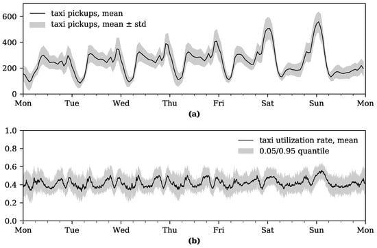
Figure 1.
Demand and supply metrics for the reference dataset: (a) hourly aggregated taxi pickups in 2018; (b) taxi utilization rate in 2018 aggregated at 5-min intervals.
5. Fleet Strategies for MoD Services
5.1. Munich Reference Strategy
In order to compare new fleet strategies, it is essential to build a reference scenario based on real-world circumstances. For this reason, the present strategy of a local taxi agency was modeled as a reference strategy. The strategy mainly resulted from the fleet management software in place. This software is an industry standard that is used in a multitude of European taxi agencies. Therefore, it was likely that similar results could be achieved in other major European cities.
In the case of Munich, the dispatching strategy relied on a heuristic based on defined sectors and ranks. For this purpose, the city was divided into 165 non-overlapping sectors and 167 taxi ranks, as displayed in Figure 2.
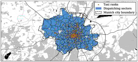
Figure 2.
Overview of sectors and ranks used for a dispatching heuristic in Munich (map tiles by Stamen Design under CC BY 3.0; data by OSM [35] under ODbL).
In general, the strategy resembled the nearest-idle-taxi dispatch approach, with fist come, first served (FCFS) sequencing on a regional scale. However, taxis awaiting customers at a rank had priority over taxis idling within the same zone. This dispatching strategy contained four major steps for assigning immediate requests to vehicles (cf. Figure 3):
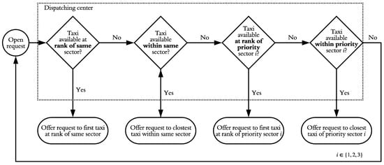
Figure 3.
Reference dispatching strategy.
- The dispatching center first assigned an incoming request to a sector based on the start location. If at least one taxi was waiting at a rank within the same sector, the request was proposed to the first taxi in the queue.
- If no taxis were present at a rank of the same sector, the ride was assigned to the closest idle taxi within the sector.
- In case of unavailability, the dispatching unit looked for idle taxis at ranks of three predefined neighboring priority sectors. The dispatching center sequentially searched for available taxis at the ranks of these sectors.
- If no taxis were present at the ranks of the neighboring sectors, open requests were offered to taxis idling in a neighboring sector.
Advance bookings with at least 15 min of reservation time were only offered to taxis waiting at a rank. Hence, the current strategy did not consider idling taxis when allocating advance bookings to vehicles.
The present fleet strategy did not involve any rebalancing of vehicles. After a customer ride, taxi drivers usually returned to sectors/ranks where they assumed the best chance of obtaining a profitable ride. As this individual choice was hard to model with the underlying dataset, the model assumed that taxi drivers returned to the nearest (shortest distance) rank following a customer drop-off.
5.2. A Profit-Maximizing Predictive Fleet-Management Strategy
As evidenced by the literature analysis, heuristic and bipartite matching models are state-of-the-art dispatching methods. To conduct matching between taxis and clients, the proposed strategy relied either on a supply-demand balancing heuristic [18] or a bipartite matching model minimizing customer waiting time. Besides these two regional dispatching methods, a dual-objective RHC-based linear optimization model was used to relocate idle vehicles among regions of over-/under-supply, based on the predicted passenger demand. Both methods were subsequently compared to each other to determine the best predictive strategy.
5.2.1. Dispatching
This analysis compared two state-of-the-art dispatching methods (NTNR, BPM) matching idle vehicles to open requests.
Supply-Demand-Balancing Strategy: NTNR
The first dispatching method used the NTNR approach applied by Maciejewski and Bischoff [18], Maciejewski et al. [19,36]. This approach differentiates between periods of over- and under-supply. If the number of idle vehicles exceeds the number of open requests (oversupply), a client is assigned to the nearest taxi in FCFS order. In contrast, if the number of open requests is higher than the amount of idle taxis (undersupply), then a taxi drives to the closest customer. This matching procedure might lead to longer waiting times for individual customers in times of undersupply, since vehicles only pick up the nearest clients. On the other hand, it decreases average waiting times when demand is high, in comparison to a simple nearest-idle-taxi heuristic [18,19,36]. The implemented NTNR algorithm had a complexity of for undersupply and respectively for oversupply, with T as the number of taxis and R as the number of requests. To utilize the potential of demand forecasts fully, this strategy was applied at regular time intervals (e.g., 1 min) to the entire set of open requests and idle vehicles. Thus, the dispatching unit periodically collected incoming requests and idle taxi data over the entire area of Munich. By conducting matching over the whole area within Munich’s borders, it was possible to increase the efficiency in terms of space. This excluded inefficient matchings, which occurred particularly at the borders of sectors such as performed by the currently practiced allocation strategy per sector. By neglecting partitioning in space, higher runtimes were accepted in favor of a better solution with respect to customer waiting time. This solution might only be practicable to a limited extent for real-time applications.
Maximum Bipartite Matching
The second dispatching strategy minimized the average customer waiting time. Here as well, idle vehicles and open requests were collected over a short period in time and matched in such a way that total waiting times were minimized. This optimization strategy is familiar from the literature as the minimum cost maximum bipartite matching technique [20,21,29]. Here, the set of incoming requests and idle vehicles was divided into two disjoint node sets. In this case, the edge cost between a vehicle and a request node represented the waiting time a client experienced when he or she was picked up by the respective taxi. A minimum cost maximum matching algorithm could be used to find the customer-vehicle allocation with the lowest total waiting time. A drawback of this approach is that several customers might suffer long waiting times in favor of the common good. From a holistic viewpoint, this approach was optimal with respect to the community. Since this study assumed constant hourly speeds, the minimized arrival times and arrival routes of taxis coincided. Thus, this technique helps a fleet operator to increase short-term profit, since the total arrival costs are minimal. However, if this results in customers who experience exceptionally long waiting times not returning as clients, this strategy can have a negative impact on an operator’s long-term profits. Similarly, a maximum bipartite matching approach was applied to the entire area of Munich for a given interval period. As mentioned above, this may lead to an increase in runtime in favor of a better matching solution. The bipartite graph made up of customer requests and idle vehicles grew in space and time, i.e., the number of nodes increased linearly, while the number of edges increased quadratically with respect to the number of incoming requests and vehicles.
5.2.2. Rebalancing
Our approach was an extension of the RHC approach formulated by Oda and Joe-Wong [7]. To recapitulate, this linear optimization located the optimal set of rebalancing flows over several discrete time horizons by maximizing the total expected reward. However, this approach rejected all requests that could not be served within a time step. Therefore, this approach was extended by considering open requests for future optimization steps. In addition, Oda and Joe-Wong [7] assumed that vehicles departed a cell at the end of a time step and arrived at the target cell at the beginning of the following time step. Since this assumption did not reflect real-world circumstances, our adaption also considered a travel time of up to one rebalancing period . Both extensions were needed to assure realistic customer servicing and supply behavior.
The resulting optimization problem could be formulated as follows: The profit to be maximized was defined as the incremental income (additionally or previously served customers) minus the supplementary costs incurred when picking up these clients. Furthermore, the space was discretized into a set of two-dimensional grid cells G. We define the supply (number of idle vehicles) within a cell, , at a given point in time t as . Similarly, we define the demand (number of open requests) in between t and as . The optimization function is limited such that no additional income is generated if the supply exceeds the demand in a cell. Consequently, up to the equilibrium of supply and demand.
By summing over all grid cells, this term counts the number of requests additionally or earlier served by rebalancing vehicles and is therefore proportional to the supplementary reward of the fleet operator. The costs of rebalancing movements result from the number of vehicles that are sent from to at a time t multiplied by variable costs, , based on the distance between and .
Since customers in undersupplied cells might be served at a later time, a weighting parameter is added to reflect the additional income from previously served requests. Hence, the weighting parameter can be interpreted as the value of time (VoT) of a customer and a driver. Furthermore, a second weighting parameter discounts the profit of future time steps in the objective function to account for prediction uncertainty. Since the customer demand in future time steps is more uncertain than the incoming demand of the next interval, near-term requests are assigned with a higher monetary value than long-term requests. In addition to maximizing the total profit over time, a set of constraints must be respected, as follows:
- The number of rebalancing vehicles leaving cell is limited by the number of available vehicles present in the respective cell. Equation 2 expresses this condition when inserting the supply definitions from below.
- All rebalancing flows must be completed within a rebalancing period . This is ensured by setting such that the cell-to-cell distance can be covered on the basis of average hourly speed . In so doing, inter-cellular distances are approximated through street distances between cell centers and .
Finally, the optimization problem is formulated as:
restricted to:
and:
Describing the vehicle supply, we define:
where is the number of idle vehicles at time t in cell and:
where:
- is the number of idle vehicles remaining from the previous time step,
- is the number of occupied vehicles becoming empty between and t,
- is the number of rebalancing vehicles from the previous time step arriving at , and is the number of vehicles, which are sent off from at the beginning of the current interval.
- Furthermore, the number of currently idle vehicles predicted to pick up a customer in region and drop off a customer in region within is estimated on the basis of the historic likelihood of possible origin-destination (OD) pairs in combination with the expected travel time of a customer ride from to depending on .
We define the customer demand over a period as:
where is the predicted number of requests for time step t, and is the amount of remaining open requests from the previous interval.
5.3. An Optimal Fleet Sizing Approach
To test the extent to which this predictive strategy could achieve the optimal fleet size, we utilized a bipartite matching fleet sizing technique. As mentioned above, this approach relies on full demand knowledge over a period . It is assumed that a customer ride can be uniquely described by the pickup and drop-off locations, and their timestamps, , such that:
Minimizing the number of taxis for a set of customer rides corresponds to solving the minimum path cover problem on the corresponding directed graph [20,29]. Thereby, the nodes of two trips and are only linked with an edge if ride can be carried out after ride by the same vehicle. This is only the case if the ride starts after the drop-off of a previous trip and if the driving distance between and can be covered within that time. Furthermore, the idle time of taxis between trips is limited by a maximum empty trip time , as follows:
Zhan et al. [29] showed that solving the minimum path cover problem corresponds to solving a maximum bipartite matching procedure on the equivalent bipartite graph. Hence, is transformed into a bipartite graph , such that the origin and destination vertexes represent two disjoint node sets (). The maximum bipartite matching problem can then be solved with a maximum flow algorithm after adding a source and sink node to with respective connections to all destination and origin nodes. Although the problem is NP-hard, it can be solved in polynomial time, for instance, by applying the Hopcroft–Karp algorithm with a complexity of where n represents the number of nodes of the bipartite graph [37].
6. Simulation Model and Parameters
6.1. Simulation Model
To compare the predictive BPM and NTNR strategies with Munich’s state-of-the-art method, this approach made use of a modular simulation model that combined independent functions; see Figure 4.
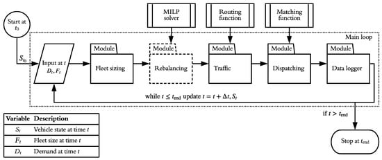
Figure 4.
Structure of the simulation model.
First of all, the fleet sizing module adjusts the number of active vehicles as a function of the input fleet size . If the current fleet size is lower than the input size, the module adds new vehicles to the simulation. If the number of active vehicles exceeds the desired fleet size, the module logs off idle taxis, until equilibrium is achieved. Then, the rebalancing module periodically directs idle vehicles to undersupplied cells by solving the MILP resulting from the linear program of Section 5.2.2 (only applies to predictive strategies). Finally, the traffic module routes the rebalancing and occupied vehicles throughout Munich’s street network. The road network used relied on data from OSM [35]. All routes (arrival, customer, and rebalancing) resulted from Dijkstra’s shortest path algorithm. Hence, the distance of every trip was minimized on the basis of the total edge length from the origin to the destination (speed differences between road classes were neglected). In the case of rebalancing vehicles, idle taxis were sent from their current location to the center node of the destination cell in accordance with the current optimal solution .
The dispatching module assigned customer requests to idle vehicles in accordance with one of the policies described in Section 5.2.1.
6.2. Simulation Parameters
For this study, a representative week in the year 2018 (11 May 2018 to 11 November 2018) was simulated. The simulated period comprised 35,602 customer requests, which reflected the average weekly demand in 2018. As the fleet of the reference dataset mainly operated in the city of Munich, only rides that started and ended within the city boundaries were considered. Furthermore, rides to and from the airport were neglected, as the reference dataset did not contain other taxi operators who mainly served this area. With a view to decreasing current costs, the current fleet size was either down- or up-scaled to the optimal fleet size. Since an analysis of the dataset showed that the real fleet size varied on a minute scale, the number of active vehicles was adjusted every 5 min so as to reflect real-world conditions.
The predicted customer demand was assumed to rely on perfect demand knowledge for computing the maximum achievable performance for the chosen algorithms as an upper bound.
The matching period not only influenced the choice of the dispatching technique, but also the dispatching behavior. The matching interval was therefore set to = 1 min both to reduce computational effort and to represent near-realistic dispatch conditions. A customer request was rejected after 20 min corresponding to the 99th percentile of observed real-world customer waiting times. Empty, idle vehicles remained at their drop-off location if no rebalancing was applied.
The main parameters of the rebalancing module were grid shape, grid size, interval length , horizons T, and frequency . For reasons of simplicity, a square grid was chosen. The finer the grid, the higher the possible performance of an optimizer. However, the number of unknown variables increased quadratically with the number of cells, since the optimizer of Section 5.2.2 had T variables with N grid cells and T optimization horizons. Spatial analysis of the origin distribution of the dataset showed that demand was concentrated at the center of Munich and decreased towards the suburbs. Consequently, the grid covered the central area with a fine resolution of 1 km × 1 km and the suburban region with a coarser resolution of 2 km × 2 km. This hybrid approach resulted in a decrease from 375 cells to 143 cells, as well as a decrease in unknowns by a factor of 7, compared to a grid with a cell size of 1 km.
The rebalancing interval must allow vehicles to reach a neighboring cell within a certain period. On the other hand, in order to limit idle times, the period should not be significantly longer than the average rebalancing durations to neighboring regions, which varied between 2 min and 10 min depending on the travel speed. Thus, a period of = 10 min was selected to allow rebalancing vehicles to reach neighboring cells within an optimization period. To avoid over- and non-optimized periods, the rebalancing frequency was also set to 10 min.
The number of control horizons was fixed to T = 2, which corresponded to a prediction horizon of 30 min. To determine the weighting parameter , a range between 0.02 and 20 was analyzed, based on realistic combinations of customer and driver VoT and possible waiting time reductions. Based on test simulations, was set to 1, since this value achieved good waiting time reductions and reasonably limited the distance of a rebalancing trip to 5.39 km.
Additionally, the travel speed of a vehicle was assumed as the hourly mean speed for the dataset for all actions (idle and customer rides).
To calculate the optimal fleet size, the request collection period was set to 1 h. This value represented a reasonable time span for the shift planning of a fleet operator. The maximum idle time of vehicles was limited by setting the inter-trip time to min.
6.3. Validation
The reference strategy was validated by comparing fleet size, average customer waiting time, and distances (arrival, idling, and customer) between the simulation and the dataset. First of all, simulated and actual fleet size coincided precisely on a temporal interval of 5 min. The distributions of simulated and real occupied distances were rather similar, but 54% of the customer trips actually made were up to 1 km longer (taxis in the dataset covered 13% more distance with a customer). One reason for this might be that taxi drivers opt for slightly longer routes than the shortest path if they allow for a higher average speed. The mean simulated idle distance of 1.3 km fell below that of 2.6 km in the dataset, since the simulated vehicles returned to the nearest rank. However, this difference was considered as acceptable as long as the waiting time and arrival distances to the customer matched. This was indeed the case, since the distribution of arrival distances was similar, i.e., simulated taxis covered only 300 m more when picking up a customer. Additionally, the simulated customer waiting time of 5.4 min reflected the actual attendance time (5.5 min) for a matching interval of 1 min. To conclude, simulated vehicles covered slightly greater distances, but the service quality almost reflected the real-world circumstances.
7. Results
7.1. Performance Based on Current Fleet Size
To evaluate the performance of the predictive strategies, the current fleet size was linearly decreased, and customer waiting time, rejected requests, and profit increase for the operator were analyzed. The waiting time was calculated as the average difference between arrival and servicing of a request over the simulated week. The profit increase for the test fleet in this study was calculated as the sum of labor and distance-based savings over the week, assuming a labor cost of 11 €/h before social security contributions and fuel plus wear and tear cost of 18.55 cts/km (based on the assumptions in [38]).
Figure 5 shows the waiting times of predictive strategies in comparison to the reference strategy. Both predictive approaches, predictive maximum bipartite matching (PR-BPM) and predictive nearest-taxi/nearest-request (PR-NTNR), were able to reduce the fleet size by 30% while maintaining the current service level. Any further decrease in fleet size would aggravate the current situation irrespective of the strategy. For small fleet sizes, the reference strategy performed significantly worse than its predictive alternatives (because it distributed vehicles evenly across the space). Table 2 confirmed that the fleet size could be reduced to no more than 70%, since customers would otherwise have to be rejected. It likewise confirmed that the predictive strategies could serve more customers than the reference approach in the event of an extreme undersupply.
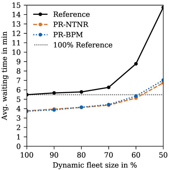
Figure 5.
Customer waiting time with respect to the current fleet size.
Table 2.
Denied requests.
Besides upholding the current service level, a strategy was expected to maximize the profit of a fleet operator on the supply side. Apart from equal labor savings, the predictive strategies showed smaller arrival distances than their non-predictive counterpart, as reflected by the income differences shown in Table 3. A 70% fleet dispatched by the PR-BPM and PR-NTNR covered 234,228 km and 236,957 km respectively, whereas the fleet controlled by the reference strategy travels 253,427 km over the course of the simulated week (Figure 6). Similarly, it showed that the operator’s incremental income increased for smaller fleets. Since fleet sizes of 60% and 50% were excluded due to the insufficient service level, an operator would opt for a PR-BPM strategy, which generated slightly more revenues than a PR-NTNR approach. The reason for this difference was that the PR-BPM minimized total arrival distances.
Table 3.
Increase in variable profit in k€.
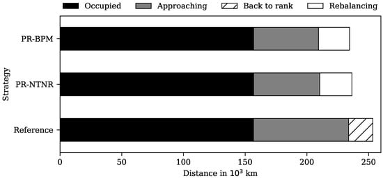
Figure 6.
Cumulative distance by taxi status for different strategies at 70% fleet size.
7.2. Performance Based on Optimal Fleet Size
Before applying the proposed fleet management methods, the optimal fleet size in the week under consideration was computed as described in Section 5.3. This hourly optimum was then fed into the fleet sizing module to adjust the number of simulated vehicles. In detail, the optimal fleet supplied only 58% of the currently provided hours, i.e., the average number of active vehicles decreased from 177 to 104. Moreover, the hourly maximum number of taxis needed fell from 292 to 188.
Again, the performance of all three policies on the basis of optimal fleet size was evaluated. Table 4 shows that both approaches were able to uphold the current waiting time level of 5.5 min for the theoretical optimum, but were not able to fulfill all customer requests. Therefore, the optimal fleet size was increased by 10% and 20%, resulting in both strategies, PR-BPM and PR-NTNR, being able to assure the current service level at 120% of the optimal fleet size. All other combinations either exceeded the threshold or were not able to serve all customers. It is interesting to note that the reference strategy rejected fewer customers than the predictive approaches. This was because its FCFS dispatching method served requests in chronological order, whereas the other strategies rejected clients during a supply shortage on Wednesday evening.
Table 4.
Waiting time in minutes (rejected requests) for the percentages of the optimal fleet size.
To conclude, the predictive approaches were not able to attain the optimum fleet size without a deterioration in service level, since the degree of information accuracy provided to the controller was too imprecise in terms of space and time. Since the number of supplied hours for 120% of the optimal fleet was roughly equal to those of 70% of the current fleet and the waiting time was no lower, there was no advantage to be had by upscaling the theoretical optimum in this case. Hence, the optimal fleet sizing approach did not increase the performance by supplying the right amount of hours at the right point in time. This may also have been because a maximum customer waiting time of 20 min was relatively high and provided for the possibility of compensating for short periods of undersupply.
8. Discussion
The aim of this study was to test the potential of a predictive strategy under a realistic MoD scenario. The performance of the proposed strategy depended first of all on the input data and parameters of the optimizer. It also relied on forecasts of pickup points; however, we assumed that the OD distribution resembled historic travel behavior (Section 5.2.2). Future models might also incorporate predictions of drop-off distributions. Furthermore, rebalancing vehicles were sent to the center of a cell. Besides modifying the shape and size of the grid cells, a higher resolution of rebalancing destinations might yield another increase in performance, which would, however, entail greater computational effort. This could, for example, be realized by predictively directing empty vehicles to the centers of demand clusters. This approach did not account for the customers’ shifting readiness to pay for a ride, e.g., clients’ willingness to pay higher prices during nighttime. This could be improved in further studies by introducing a time-dependent reward parameter .
Secondly, the reference model was not able to reproduce the idling behavior of taxi drivers accurately. To incorporate this, we would need to take into account the individual decision making process of a single driver. Nevertheless, we always compared the results with the simulated reference model rather than actual values of the real-world dataset, in order to exclude side effects and possible model inaccuracies. Furthermore, we relied on a batch matching technique, with a period of = 1 min, although this could be reduced further to simulate real-time dispatching.
Finally, we found that there was no advantage of upscaling the perfect fleet size by reducing the current amount of vehicles in the week investigated. This result might vary if the reject period of 20 min changes. The importance of a predictive strategy and accurate vehicle positioning might increase if the customers’ willingness to wait for a taxi decreases. Besides this simple percentage-based modification, we aim to test fleet scaling methods that integrated demand forecasts.
The present simulation model lacked computational efficiency. In order to compute simulations over a long-term period (one year), we plan to integrate our algorithms into a more efficient and scalable framework such as amodeus [23].
The presented fleet strategy assumed that fleet operators were able to control actions taxi drivers usually decide as individuals. Even if this strategy offered cost-reductions and operational benefits in a global perspective, not all drivers would profit from this approach. For example, drivers who had high turnovers, because they anticipated demand or adapted quickly to dynamic changes, were now forced to act in the interest of the global optimum. Fleet operators may therefore rethink their salary models to compensate such effects.
This study did not reflect on the dynamic reassignment of taxis. It has to be investigated to what extent dynamic reassignment of customers is beneficial to further reduce waiting times and operational costs.
9. Conclusions
A literature analysis of predictive fleet management strategies, including fleet sizing, was conducted for MoD scenarios. None of the existing predictive approaches were tested in conjunction with a dynamic, time-varying fleet size. Our contribution was to improve an existing model and apply it to different time-dependent fleet sizes, as well as to the optimal fleet size, of a large-scale taxi dataset.
As a result, it was found that the current fleet size could be reduced by 30% without aggravating the current service level. By applying a PR-BPM model, a fleet operator could save up to 120,670€ per week and reduce the fleet’s total distance by 19,199 km. However, the simulation results also showed that the the optimum fleet size could only be attained to a limited extent using the proposed strategies. Both predictive strategies in conjunction with the theoretical fleet minimum upscaled by 20% were able to serve all customers without increasing the present waiting time threshold.
We further intend to show that this reduction potential also holds for other periods of the year, for instance by performing simulations of low-demand (e.g., Christmas) and high-demand periods (e.g., Oktoberfest). Additionally, we aim to test the controller in combination with demand forecasts of an LSTM neural network to evaluate the extent to which prediction accuracy influences the optimizer’s performance. This work represents a first step towards testing the potential of predictive strategies for dynamic fleet sizes based on a real-world dataset.
Author Contributions
M.W. as the first author primarily developed the research question and made an essential contribution to the overall structure of the software, the methodology of the algorithms, and the validation of the data. Conceptualization, M.W. and L.N.; data curation, M.W.; formal analysis, M.W. and L.N.; investigation, M.W. and L.N.; methodology, M.W.; resources, M.W.; software, M.W. and L.N.; supervision, M.W. and M.L.; validation, M.W. and L.N.; visualization, M.W.; writing, original draft, M.W. and L.N.; writing, review and editing, M.W., L.N., and M.L. All authors have read and agreed to the published version of the manuscript.
Funding
The Chair of Automotive Technology at the Technical University of Munich funded the project independently.
Acknowledgments
The authors would like to thank IsarFunk Taxizentrale GmbH & Co. KG for providing useful taxi data.
Conflicts of Interest
The authors declare no conflict of interest.
Abbreviations
| MoD | mobility-on-demand |
| MaaS | mobility as a service |
| GNSS | Global Navigation Satellite System |
| RHC | receding horizon control |
| DQN | deep Q network |
| ILP | integer linear program |
| MILP | mixed integer linear program |
| FCD | floating car data |
| LSTM | long short-term memory |
| FCFS | fist come, first served |
| VoT | value of time |
| OD | origin-destination |
| BPM | maximum bipartite matching |
| NTNR | nearest-taxi/nearest-request |
| PR-BPM | predictive maximum bipartite matching |
| PR-NTNR | predictive nearest-taxi/nearest-request |
| OSM | Open Street Map |
Nomenclature
| G | Set of grid cells |
| N | Number of grid cells |
| Matching period | |
| Rebalancing period | |
| Rebalancing frequency | |
| T | Number of control horizons |
| Total number of available vehicles in cell i at t | |
| Number of open requests in cell i between t and | |
| Number of predicted requests in cell i between t and | |
| Number of rebalancing vehicles sent from cell i to j at t | |
| Number of already idle vehicles in cell i at t | |
| Number of occupied vehicles turning idle in cell i between and t | |
| Variable cost for traveling from cell i to j | |
| Weighting parameter | |
| Probability distribution of the destination cell j based on starting cell i at time t | |
| Street distance between cell centers and | |
| Discount factor | |
| Vehicle speed at time t | |
| Pickup location of ride i | |
| Drop-off location of ride i | |
| Pickup time of ride i | |
| Drop-off time of ride i | |
| Optimization horizon | |
| Street distance between the drop-off location of ride i and the pickup location of ride j | |
| Maximum trip connection time |
References
- Keeney, T. Mobility-As-a-Service: Why Self-Driving Cars Could Change Everything. Available online: https://research.ark-invest.com/self-driving-cars-white-paper (accessed on 16 April 2020).
- Willmroth, J. Freie Fahrt für Freie Taxler. Available online: https://www.sueddeutsche.de/auto/fahrdienste-taxi-uber-1.4336689 (accessed on 19 February 2020).
- MarketsandMarkets. Fleet Management Market. Available online: https://www.marketsandmarkets.com/updatedreport/fleet-management-market-1020.asp (accessed on 22 February 2020).
- NYC Taxi & Limousine Commission. TLC Trip Record Data. Available online: https://www1.nyc.gov/site/tlc/about/tlc-trip-record-data.page (accessed on 16 April 2020).
- Piorkowski, M.; Sarafijanovic-Djukic, N.; Grossglauser, M. CRAWDAD Dataset Epfl/Mobility. 2009. Available online: https://crawdad.org/epfl/mobility/20090224 (accessed on 24 February 2019).
- Data.world. Uber Pickups in NYC. Available online: https://data.world/data-society/uber-pickups-in-nyc (accessed on 16 April 2020).
- Oda, T.; Joe-Wong, C. MOVI: A Model-Free Approach to Dynamic Fleet Management. In Proceedings of the IEEE INFOCOM 2018-IEEE Conference on Computer Communications, Honolulu, HI, USA, 16–19 April 2018. [Google Scholar] [CrossRef]
- Xu, J.; Rahmatizadeh, R.; Boloni, L.; Turgut, D. Taxi Dispatch Planning via Demand and Destination Modeling. In Proceedings of the 2018 IEEE 43rd Conference on Local Computer Networks (LCN), Chicago, IL, USA, 1–4 October 2018. [Google Scholar] [CrossRef]
- Miao, F.; Han, S.; Lin, S.; Stankovic, J.A.; Zhang, D.; Munir, S.; Huang, H.; He, T.; Pappas, G.J. Taxi Dispatch With Real-Time Sensing Data in Metropolitan Areas: A Receding Horizon Control Approach. IEEE Trans. Autom. Sci. Eng. 2016, 13, 463–478. [Google Scholar] [CrossRef]
- Tsao, M.; Iglesias, R.; Pavone, M. Stochastic Model Predictive Control for Autonomous Mobility on Demand. In Proceedings of the 2018 21st International Conference on Intelligent Transportation Systems (ITSC), Maui, HI, USA, 4–7 November 2018. [Google Scholar] [CrossRef]
- Dandl, F.; Hyland, M.; Bogenberger, K.; Mahmassani, H.S. Evaluating the impact of spatio-temporal demand forecast aggregation on the operational performance of shared autonomous mobility fleets. Transportation 2019, 46, 1975–1996. [Google Scholar] [CrossRef]
- Pavone, M.; Smith, S.; Frazzoli, E.; Rus, D. Load balancing for mobility-on-demand systems. In Robotics: Science and Systems VII; The MIT Press: Cambridge, MA, USA, 2012; pp. 249–256. [Google Scholar]
- Zhang, R.; Pavone, M. Control of robotic mobility-on-demand systems: A queueing-theoretical perspective. Int. J. Robot. Res. 2015, 35, 186–203. [Google Scholar] [CrossRef]
- Iglesias, R.; Rossi, F.; Wang, K.; Hallac, D.; Leskovec, J.; Pavone, M. Data-Driven Model Predictive Control of Autonomous Mobility-on-Demand Systems. In Proceedings of the 2018 IEEE International Conference on Robotics and Automation (ICRA), Brisbane, Australia, 21–25 May 2018. [Google Scholar] [CrossRef]
- Tsao, M.; Milojevic, D.; Ruch, C.; Salazar, M.; Frazzoli, E.; Pavone, M. Model Predictive Control of Ride-sharing Autonomous Mobility-on-Demand Systems. In Proceedings of the 2019 International Conference on Robotics and Automation (ICRA), Montreal, QC, Canada, 20–24 May 2019. [Google Scholar] [CrossRef]
- Miller, J.; How, J.P. Predictive positioning and quality of service ridesharing for campus mobility on demand systems. In Proceedings of the 2017 IEEE International Conference on Robotics and Automation (ICRA), Singapore, 29 May–3 June 2017. [Google Scholar] [CrossRef][Green Version]
- Alonso-Mora, J.; Wallar, A.; Rus, D. Predictive routing for autonomous mobility-on-demand systems with ride-sharing. In Proceedings of the 2017 IEEE/RSJ International Conference on Intelligent Robots and Systems (IROS), Vancouver, BC, Canada, 24–28 September 2017. [Google Scholar] [CrossRef]
- Maciejewski, M.; Bischoff, J. Large-scale Microscopic Simulation of Taxi Services. Procedia Comput. Sci. 2015, 52, 358–364. [Google Scholar] [CrossRef]
- Maciejewski, M.; Bischoff, J.; Nagel, K. An Assignment-Based Approach to Efficient Real-Time City-Scale Taxi Dispatching. IEEE Intell. Syst. 2016, 31, 68–77. [Google Scholar] [CrossRef]
- Vazifeh, M.M.; Santi, P.; Resta, G.; Strogatz, S.H.; Ratti, C. Addressing the minimum fleet problem in on-demand urban mobility. Nature 2018, 557, 534–538. [Google Scholar] [CrossRef] [PubMed]
- Hörl, S.; Ruch, C.; Becker, F.; Frazzoli, E.; Axhausen, K. Fleet operational policies for automated mobility: A simulation assessment for Zurich. TRansp. Res. Part C Emerg. Technol. 2019, 102, 20–31. [Google Scholar] [CrossRef]
- Ruch, C.; Hörl, S.; Hakenberg, J.; Frazzoli, E. The Impact of Fleet Coordination on Taxi Operations. 2019. Available online: https://www.research-collection.ethz.ch/handle/20.500.11850/379519 (accessed on 18 June 2020).
- Ruch, C.; Horl, S.; Frazzoli, E. AMoDeus, a Simulation-Based Testbed for Autonomous Mobility-on-Demand Systems. In Proceedings of the 2018 21st International Conference on Intelligent Transportation Systems (ITSC), Maui, HI, USA, 4–7 November 2018. [Google Scholar] [CrossRef]
- Ruch, C.; Gächter, J.; Hakenberg, J.; Frazzoli, E. The +1 Method Model-Free Adaptive Repositioning Policies for Robotic Multi-Agent Systems. 2019. Available online: https://www.research-collection.ethz.ch/handle/20.500.11850/322945 (accessed on 18 June 2020).
- Seow, K.T.; Dang, N.H.; Lee, D.H. Towards An Automated Multiagent Taxi-Dispatch System. In Proceedings of the 2007 IEEE International Conference on Automation Science and Engineering, Scottsdale, AZ, USA, 22–25 September 2007. [Google Scholar] [CrossRef]
- Seow, K.T.; Dang, N.H.; Lee, D.H. A Collaborative Multiagent Taxi-Dispatch System. IEEE Trans. Autom. Sci. Eng. 2010, 7, 607–616. [Google Scholar] [CrossRef]
- Gao, Y.; Jiang, D.; Xu, Y. Optimize taxi driving strategies based on reinforcement learning. Int. J. Geogr. Inf. Sci. 2018, 32, 1677–1696. [Google Scholar] [CrossRef]
- Xu, Z.; Li, Z.; Guan, Q.; Zhang, D.; Li, Q.; Nan, J.; Liu, C.; Bian, W.; Ye, J. Large-Scale Order Dispatch in On-Demand Ride-Hailing Platforms. In Proceedings of the 24th ACM SIGKDD International Conference on Knowledge Discovery & Data Mining, London, UK, 19–23 August 2018. [Google Scholar] [CrossRef]
- Zhan, X.; Qian, X.; Ukkusuri, S.V. A Graph-Based Approach to Measuring the Efficiency of an Urban Taxi Service System. IEEE Trans. Intell. Transp. Syst. 2016, 17, 2479–2489. [Google Scholar] [CrossRef]
- Zhu, C.; Prabhakar, B. Reducing inefficiencies in taxi systems. In Proceedings of the 2017 IEEE 56th Annual Conference on Decision and Control (CDC), Melbourne, Australia, 12–15 December 2017. [Google Scholar] [CrossRef]
- Hörl, S.; Ruch, C.; Becker, F.; Frazzoli, E.; Axhausen, K.W. Fleet control algorithms for automated mobility: A simulation assessment for Zurich. In Proceedings of the Transportation Research Board 97th Annual Meeting, Washington, DC, USA, 7–11 January 2018. [Google Scholar] [CrossRef]
- Bischoff, J.; Maciejewski, M. Simulation of City-wide Replacement of Private Cars with Autonomous Taxis in Berlin. Procedia Comput. Sci. 2016, 83, 237–244. [Google Scholar] [CrossRef]
- Spieser, K.; Treleaven, K.; Zhang, R.; Frazzoli, E.; Morton, D.; Pavone, M. Toward a Systematic Approach to the Design and Evaluation of Automated Mobility-on-Demand Systems: A Case Study in Singapore. In Road Vehicle Automation; Springer International Publishing: Berlin, Germany, 2014; pp. 229–245. [Google Scholar] [CrossRef]
- Jäger, B.; Wittmann, M.; Lienkamp, M. Analyzing and Modeling a City’s Spatiotemporal Taxi Supply and Demand: A Case Study for Munich. J. Traffic Logist. Eng. 2016, 4, 147–153. [Google Scholar] [CrossRef]
- OpenStreetMap Contributors. Map Data. 2020. Available online: https://download.geofabrik.de/europe/germany/bayern.html (accessed on 16 April 2020).
- Maciejewski, M.; Salanova, J.M.; Bischoff, J.; Estrada, M. Large-scale microscopic simulation of taxi services. Berlin and Barcelona case studies. J. Ambient. Intell. Humaniz. Comput. 2016, 7, 385–393. [Google Scholar] [CrossRef][Green Version]
- Hopcroft, J.E.; Karp, R.M. An n5/2 algorithm for maximum matchings in bipartite graphs. In Proceedings of the 12th Annual Symposium on Switching and Automata Theory (swat 1971), East Lansing, MI, USA, 13–15 October 1971. [Google Scholar] [CrossRef]
- Bundesverband Taxi und Mietwagen e.V. BZP Geschäftsbericht 2017/2018; Technical Report; Bundesverband Taxi und Mietwagen e.V.: Frankfurt am Main, Germany, October 2019. [Google Scholar]
© 2020 by the authors. Licensee MDPI, Basel, Switzerland. This article is an open access article distributed under the terms and conditions of the Creative Commons Attribution (CC BY) license (http://creativecommons.org/licenses/by/4.0/).