Performance Analysis of Cooperative Sensing over Time-Correlated Rayleigh Channels in Vehicular Environments

Abstract

Spectrum starvation is a key challenge for wireless services and applications in vehicular networks with serious negative implications for traffic safety and transportation efficiency. As a promising solution, cognitive radio (CR) allows CR-enabled vehicles to access the spectrum holes of primary users (PUs) in an opportunistic manner, but requires a robust sensing mechanism to provide adequate protection for PUs. However, highly dynamic environments make spectrum sensing an increasingly difficult problem. For example, vehicular communications are subject to multipath fading due to vehicle mobility. In this paper, the wireless channels in vehicular environments are considered to be subject to time-correlated Rayleigh fading. To facilitate the analysis, temporal correlation could be classified into complete correlation, partial correlation and complete independence according to the degree of correlation. The performance of cooperative sensing scheme is investigated for soft fusion (SF) and hard fusion (HF) approaches. The simulation results are presented to verify our theoretical analysis for varying conditions and scenarios. The results indicate that the detecting performance could be importantly influenced by channel correlation, which can be improved by vehicles’ cooperation.

1. Introduction

The concept of vehicular communication networking has fascinated researchers working in various fields because it has the ability and the potential to enhance vehicular safety and transportation efficiency. And for this, national governments have contributed licensed spectrum (a 75 MHz bandwidth in the 5.85–5.925 GHz) to sustain and develop the dedicated short range communications (DSRC) [1]. With an increasing number of vehicles, there is an explosively increasing demand for the radio spectrum resources to satisfy their requirements of future wireless communications. Spectrum deficiency has become so strong pressure and a tremendous challenge in vehicular networks.

In light of the challenge, cognitive radio (CR) [2] incorporated into vehicular networks has been proposed to alleviate the pressure from the increasing demand for the radio spectrum. We call such a vehicular networks with CR capability as a cognitive vehicular network (CVN), as well as vehicles with CR capability as secondary vehicular users (SVUs) [3]. In a CVN, the SVUs need to accurately understand the environmental changes to actively seek out the additional idle spectrum without interfering the incumbent license holders’ usage. However, in the most common scenario, there is no coordination and collaboration between primary users (PUs) and SVUs. To efficiently avoid interfering with PUs and reutilize the spectrum holes, the SVUs should have the ability to quickly and reliably sense the presence or absence of PUs. Ideally, we hope that they must immediately vacate the radio channels as soon as PUs are detected within SUs’ transmission range. Since that is so, it follows that spectrum sensing is a key design issue of CVNs.

1.1. Related Work

Over the last several years, we have witnessed spectrum sensing has been widely investigated [4,5,6]. Individual spectrum sensing is always compromised by multipath fading, shadowing and noise uncertainty. For this, cooperative spectrum sensing [7,8] has received more attention as it can take further advantage of both spatial and temporal diversity, and thereby garner better sensing accuracy and efficiency in the face of deep fading. However, it is worth noting that most of these efforts are focused primarily on a static network and scenario. As a result, they are much less suitable in a vehicular environment. Furthermore, it is all because it is of great importance to take into account the dynamic properties of cognitive environments and the environmental impact on radio propagation when designing sensing scheme for vehicle users [3,9].

So far, Spectrum sensing in vehicular environments have been investigated in some fundamental works [10,11,12,13,14,15,16,17,18,19,20,21]. The work in [10] is among the first to study the influence of mobility on spectrum sensing in a joint optimization framework for sensor cooperation and sensing scheduling. The work in [11] takes advantage of SVU mobility to enhance the detection performance under the emulation attack. In [12], the authors introduced a well-coordinated mechanism of information-adaptive spectrum sensing in CVNs, which can reach a near perfect compromise between local and collaborative sensing. The work in [13] proposed a Bayesian machine learning based cooperative sensing framework in a mobile heterogeneous networks. The proposed framework aims at reducing the number of SVUs participating cooperation. The work in [14] proposed a novel cooperative sensing scheme based on compressive sensing and clustering in order to reduce the processing time while achieving high detection. In [15], it presented a voting-based distributed collaborative sensing strategy, in which the adaptive detection threshold is optimized through the adoption of a computationally efficient numerical approach. The work in [16] proposed a cooperative mechanism with double adjustable thresholds, which has the potential to adjust to the varying environmental conditions while keeping up levels of detection. The work in [17] explored an energy detection based CSS scheme in a CVN with the uniform speed of the PU and SVUs. A distance-dependent distribution function is developed first to find the probability of an SU resides in a specific coverage of the PU transmission zone. This distribution function is then used in deducing the expression of false-alarm and detection probability using majority rule at the fusion center. In addition, the performance of cooperative spectrum sensing were studied over Nakagami-m Fading Channels [18,19] and generalized $\kappa -\mu$ fading [20,21]. For a more in-depth discussion of spectrum sensing in CVNs, the reader is referred directly to [22].

However, there are still many potential problems, which are worthy of thoroughly researching. Most of these previous works either focused mainly on robust technical design of CVNs from the network designer’s angle, or overlooked the effect of temporal correlation due to the mobility of vehicles and the time-variant characteristics of channels.

1.2. Contributions

In this paper, we consider an infrastructure-aided cooperative sensing scheme in cognitive vehicular networks. We treat the PU signal as unknown and deterministic with a known power and the sensing channels as random with a time-correlated Rayleigh distribution. The main contributions and significance of this paper are threefold.

Firstly, we consider a large-scale PUs detection in the infrastructure-aided CVNs based on mutual benefit and acquiring a win-win situation by allowing the back SVUs take advantage of the spectral state information obtained by the front SVUs’ sensing.

Secondly, the radio channel has a major effect on the detecting performance. In this paper, we model the sensing channels in CVNs by a time-correlated Rayleigh fading. Furthermore, in order to facilitate the analysis, the temporal correlation is classified into completely correlated (${\mathcal{C}}_1$), partially correlated (${\mathcal{C}}_2$) and completely independent (${\mathcal{C}}_3$) according to the degree of correlation.

Thirdly, we will consider collaboration strategy, including both soft fusion and hard fusion. The detection performances are evaluated through theoretical analysis or Monte Carlo simulation. The obtained results indicate that radio channel correlation can apparently deteriorate the detection performance. However, the fast time-varying characteristic of sensing channels can give us an opportunity to obtain temporal diversity provided that a proper sensing technique is adopted.

1.3. Organization and Notation

The remainder of the paper is organized as follows. Section 2 describes the detailed system model and assumptions on spectrum sensing in vehicular environments. Then, we mathematically analyze the performance of spectrum sensing over correlated Rayleigh fading in Section 3. The numerical evaluation and simulating results are presented and discussed in Section 4. At last, we conclude our observations and future work in Section 5.

Throughout this paper on the performance, we will declare the local probabilities of false alarm, miss detection, and detection as $P_f$, $P_m$, and $P_d$, respectively, whereas their global probabilities at the FC will be represented by $P_F$, $P_M$, and $P_D$ for soft fusion and $Q_F$, $Q_M$, and $Q_D$ for hard fusion. $X\sim \mathcal{C}\mathcal{N}\left({\mu }_1,{\sigma }_1^2\right)$ denotes that X is a complex Gaussian distribution with mean ${\mu }_1$ and co-variance ${\sigma }_1^2$, while $Y\sim \mathcal{N}\left({\mu }_2,{\sigma }_2^2\right)$ denotes that Y is a real Gaussian distribution with mean ${\mu }_2$ and variance ${\sigma }_2^2$. Let ${\mathcal{H}}_0$ and ${\mathcal{H}}_1$ denote the null and alternative hypotheses associated to the absence and presence of PUs in the considered band, respectively. The probability that the PU is absent is $P\left({\mathcal{H}}_0\right)$ and present is $P\left({\mathcal{H}}_1\right)$.

2. System Description

This section is divided into four subsections, which clearly expound network model, sensing channel model, local and cooperative sensing model in the CVNs, and some assumptions made in the study.

2.1. Network Model

Without loss of generality, we consider an infrastructure-aided CVN consisting of a PU, a roadside unit (which is also referred to as fusion center (FC)) and multiple SVUs, as Figure 1 shows. There is usually an assumption that the SVUs in a steady traffic flow move with a relative steady velocity, so that the network topology appears to be stable in a certain duration as well despite the SVUs move. The roadside unit coordinates SVUs to participate in cooperative spectrum sensing in a synchronous way. The time period is partitioned into frames. Each frame is designed with periodic spectrum sensing for the CVN. Figure 2 shows that the frame structure consists of three phases: a sensing phase, a reporting phase, and a transmission phase. When vehicles are traveling on the road, the following steps show the procedure of the collaborative sensing.

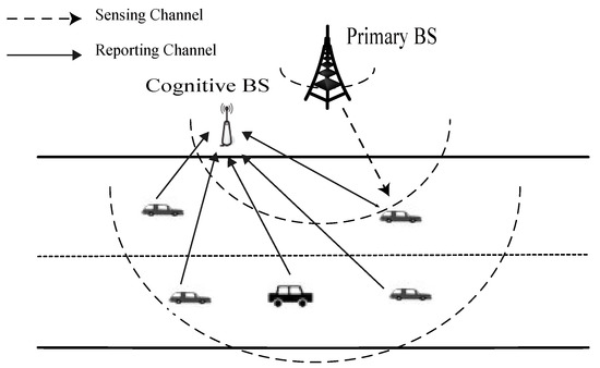
Figure 1. Cooperative spectrum sensing in a cognitive vehicular network. The wireless links between the PU and SVUs are referred to as the sensing channels, whereas the links between the SVUs and FC are the reporting channels.

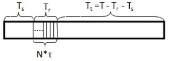
Figure 2. Frame structure for CVNs with periodic spectrum sensing ($T_s$: sensing slot duration; $T_r=N\tau$: reporting slot duration; $T_t=T-T_s-T_r$: data transmission slot duration).

Step 1:

Each SVU senses the PU by means of energy detector in the local sensing slot, and then sends their local information (energy statistics or binary decisions) to the nearby FC through the control channel in the reporting slot.

Step 2:

The FC receives the local information and combines them to reach a global decision on the availability of licensed bands for future passing SVUs.

Step 3:

If the absence of the PU is recognized, the FC feeds back the transmission ACK to all the SVUs in the current cell, and thus the SVUs can send data in the transmission slot.

Step 4:

Or else, if the PU is detected, the FC feeds back the stop ACK to the SVUs, and thus the SVUs wait for the next sensing cycle.

2.2. Sensing Channel Model

In this scenario, we consider the sensing channels, which have no correlation in space but are temporally correlated following the Jakes’ model of land mobile fading channel [23]. Let $\rho$ denotes the temporal correlation coefficient, which satisfies

$$\begin{array}{c}\hfill \rho ={\mathcal{J}}_0\left(2\pi f_d{T}_s\theta \right),\end{array}$$

(1)

where ${\mathcal{J}}_0(·)$ is defined by the $zero$th-order Bessel function of the first kind [24], $f_d$ is the maximal Doppler shift of the CR user, $T_s$ is the sampling interval, and $\theta$ is the time interval.

The time correlation is completely determined by $f_d{T}_s$, like the one depicted in Figure 3. For small values of $f_d{T}_s(<0.001)$, $\rho$ approaches 1, the fading has a strong correlation structure in time. Conversely, as $f_d{T}_s$ increases $(>0.03)$, $\rho$ approaches 0, yet with extremely weak correlation (or completely random). To facilitate the analysis later, we can employ three suitable model, ${\mathcal{C}}_1$, ${\mathcal{C}}_2$ and ${\mathcal{C}}_3$, as follows

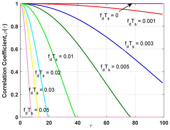
Figure 3. The correlation coefficient for various $f_d{T}_s$.

${\mathcal{C}}_1$:

For smaller values of $f_d{T}_s$ $(<0.001)$, the channel is quasi-static (at least, during a sensing period of time).

${\mathcal{C}}_2$:

When $f_d{T}_s$ is small $(<0.03)$, the channel is time-correlated.

${\mathcal{C}}_3$:

For larger values of $f_d{T}_s$ $(>0.03)$, the channel is completely random time-varying.

It is important to stress that ${\mathcal{C}}_1$ and ${\mathcal{C}}_3$ can be viewed as special cases of time-correlated channel. Without loss of generality, we postulate that the vehicles move independently, so that the sensing channels for different SVUs are independent of each other.

2.3. Local Sensing Model

In general, spectrum sensing is considered as a binary hypothesis testing issue with hypotheses ${\mathcal{H}}_0$ and ${\mathcal{H}}_1$. In the following, we firstly take account of local sensing over a sensing interval of K sampling observations at the i-th SVU.

Under these hypotheses, the received observation at the kth time instant can be formulated as, respectively

$$\begin{array}{c}\hfill \begin{array}{cc}{\mathcal{H}}_0:\hfill & r_i\left(k\right)=n_i\left(k\right)\hfill \\ {\mathcal{H}}_1:\hfill & r_i\left(k\right)=h_i\left(k\right)s\left(k\right)+n_i\left(k\right),\hfill \end{array}\end{array}$$

(2)

where $r_i\left(k\right)$ denotes the signal received by the SVU, $s\left(k\right)$ denotes the baseband-equivalent signal transmitted by the PU, with the power $P_0=\frac{1}{K}{\sum }_{k=1}^K|s\left(k\right){|}^2$, $h_i\left(k\right)$ denotes the sensing channel gain with fading power $\mathbb{E}\left\{h_i\left(k\right){|}^2\right\}=1$, and $n_i\left(k\right)$ denotes white and circularly symmetric complex Gaussian noise with mean zero and variance ${\sigma }_n^2$, i.e., $n_i\left(k\right)\sim \mathcal{C}\mathcal{N}(0,{\sigma }_n^2)$. Moreover, it is also assumed that $s\left(k\right)$ and $h_i\left(k\right)$ are statistically independent for all SVUs, which is entirely rational from actual condition point of view. In the CVN, the average SNR measured at the secondary receiver is ${\eta }_0=\frac{P_0}{{\sigma }_n^2}$.

For local sensing, there are three fundamental sensing techniques namely energy detection, cyclostationary feature detection and matched filter detection. The authors in [6,25] provide a comprehensive comparison among the three sensing techniques. Among them, cyclostationary feature detection and matched filter detection can guarantee better detection performance. However, due to their implementation complexity and need for priori knowledge of the PU signal, the two detection technique are seldom implemented for spectrum sensing in CVNs. So it follows that energy detector [26,27] become a good choice for vehicular environments as a result of its simplicity, low computational cost, and needing no priori information about the PU signal.

In general, the local test statistic related to the energy detector at the ith SVU, denoted as $e_i$, is basically an estimate of received signal power which is represented as:

$$\begin{array}{c}\hfill e_i=\frac{1}{K}\sum _{k=1}^K|r_i{\left(k\right)|}^2,\end{array}$$

(3)

where $\left|·\right|$ denotes the absolute operation.

To make a decision on the spectrum’s occupancy state, the local statistic $e_i$ is compared with a predefined threshold ${\lambda }_{local}$. In other words, the decision rule used by energy detector can be expressed as

$$\begin{array}{c}\hfill u_i=\left\{\begin{array}{cc}1\hfill & \mathrm{if}{e}_i\ge {\lambda }_{local}\hfill \\ 0\hfill & \mathrm{if}{e}_i<{\lambda }_{local}\hfill \end{array}\right..\end{array}$$

(4)

2.4. Cooperative Sensing Model

Cooperative among the SVUs in different positions can improves the spectrum sensing performance. In this paper, we will investigate cooperative sensing including both soft fusion [28,29] and hard fusion [30,31]. In soft fusion, all cooperative SVUs transmit their complete local test statistics directly to the FC. The local test statistics is normally quantized by a large number of bits that is enough to ignore the resulting quantization distortion. In hard fusion, each SVU makes its own individual binary decision, and reports only 1-bit binary decision to the FC. Therefore, we denote the time slot required for reporting the sensing result in hard scheme by $\tau =1$ and in soft scheme by $\tau =B(>1)$. Clearly, the soft fusion scheme can acquire better sensing robustness and reliability at the expense of the reporting overhead while the hard fusion can effectually reduce the required control channel bandwidth with potentially compromised sensing sensitivity due to the message loss.

For fusion rule at the FC, we assume Equal Gain Combining (EGC) for cooperative sensing. As widely known, EGC is a low complexity diversity scheme and approaches near-optimal performance without the need of channel estimation.

Let N denote the number of SVUs collaborating. For simplicity, we make assumptions that the dedicated control channels between SVUs and FC are error-free, and the latencies can be inappreciable as well [32]. Once the FC receives $\left\{e_i\left(u_i\right),i=1,\cdots N\right\}$, we adopt the following linear fusion rule

$$\begin{array}{c}\hfill {\Lambda }_c=\sum _{i=1}^N{e}_i\left(u_i\right)\left\{\begin{array}{cc}\ge {\lambda }_c& {\mathcal{H}}_1\\ <{\lambda }_c& {\mathcal{H}}_0\end{array}\right.\end{array}$$

(5)

where ${\Lambda }_c$ denotes the linear combination of the local test statistics, ${\lambda }_c$ denotes the global threshold of cooperative sensing, and the subscript $c\in \{soft,hard\}$ corresponds to cooperative sensing based on SF or HF.

3. Performance Analysis

Two important metrics for assessing the efficiency of spectrum sensing techniques are the probability of false alarm and the probability of detection. This section thoroughly investigates the detecting performances of spectrum sensing in terms of the probabilities of false alarm $P_f\left(P_F,Q_F\right)$ and detection $P_d\left(P_D,Q_D\right)$ at single secondary user (fusion center) under the considered model.

3.1. False Alarm and Detection for ED-Based Local Sensing

In this subsection, let us focus on the calculation of the average probabilities of false alarm (${\overline{P}}_f$) and detection (${\overline{P}}_d$) for local sensing under time-correlated Rayleigh sensing channel.

For a high number of sensing observations K, on the basis of the Central Limit Theorem (CLT), the local test statistic $e_i$ given by (3) can be well modeled by a normal or Gaussian distribution under either ${\mathcal{H}}_0$ or ${\mathcal{H}}_1$ [26]. To be specific, the probability density function (PDF) of $e_i$ at individual SVU can be compactly characterized by

$$\begin{array}{c}\hfill e_i\sim \left\{\begin{array}{cc}\mathcal{N}\left({\sigma }_n^2,\frac{1}{K}{\sigma }_n^4\right)& {\mathcal{H}}_0\\ \mathcal{N}\left(\left(1+{\eta }_i\right){\sigma }_n^2,\frac{\left(1+2{\eta }_i\right)}{K}{\sigma }_n^4\right)& {\mathcal{H}}_1\end{array}\right.,\end{array}$$

(6)

where

$${\eta }_i=\frac{1}{K}\sum _{k=1}^K{\left|h_i\left(k\right)\right|}^2\frac{P_0}{{\sigma }_n^2},$$

(7)

represents the instantaneous SNR measured at the i-th SVU within the current sensing period. It is straightforward to see that ${\eta }_i$ is a random variable which varies from one (sensing) interval to another. This is due to the fact that it generally hinges upon the fading variations of sensing channels.

In the above discussed case, for an individual SVU i, the probabilities of false alarm and detection can be represented by the following formulas, respectively

$$\begin{array}{cc}\hfill P_{f,i}\left({\lambda }_{local}\right)& =\mathrm{Pr}\left\{e_i\ge {\lambda }_{local}|{\mathcal{H}}_0\right\}\hfill \\ \hfill & =\mathcal{Q}\left(\frac{{\lambda }_{local}-{\sigma }_n^2}{\sqrt{\frac{1}{K}}{\sigma }_n^2}\right),\hfill \end{array}$$

(8)

$$\begin{array}{cc}\hfill P_{d,i}({\lambda }_{local},{\eta }_i)& =\mathrm{Pr}\left\{e_i\ge {\lambda }_{local}|{\mathcal{H}}_1\right\}\hfill \\ \hfill & =\mathcal{Q}\left(\frac{{\lambda }_{local}-(1+{\eta }_i){\sigma }_n^2}{\sqrt{\frac{1+2{\eta }_i}{K}}{\sigma }_n^2}\right).\hfill \end{array}$$

(9)

where $\mathrm{Pr}\left\{·\right\}$ is the cumulative distribution dunction (CDF), and $\mathcal{Q}\left(t\right)$ is defined by the complementary cumulative distribution function (CDF) of standard Gaussian, i.e.,

$$\begin{array}{c}\hfill \mathcal{Q}\left(t\right)=\frac{1}{\sqrt{2\pi }}{\int }_t^{+\infty }{e}^{-\frac{y^2}{2}}dy.\end{array}$$

(10)

Distinctly, $P_{f,i}$ given by (8) is irrelevant to the instantaneous SNR ${\eta }_i$, and while $P_{d,i}$ given by (9) is a conditional probability relying too heavily on ${\eta }_i$, for all i. As a result, the average probability of detection, ${\overline{P}}_d$, could be evaluated through integrating the $P_{d,i}$ over the SNR fading distribution, or quantify the quality of each channel by its corresponding average received SNR.

It is also observed that there is a clear trade-off between $P_{f,i}$ and $P_{d,i}$. According to different frameworks, different detection criteria are claimed to balance the performance. In the Neyman–Pearson criterion, $P_{f,i}$ is fixed as the constraint of the detection problem. Thus, ${\lambda }_{local}$ can be adjusted to ensure the predefined probability (${\overline{P}}_f$), being expressed as follows

$$\begin{array}{c}\hfill {\lambda }_{local}=\left(\sqrt{\frac{1}{K}}{\mathcal{Q}}^{-1}\left({\overline{P}}_f\right)+1\right){\sigma }_n^2,\end{array}$$

(11)

where ${\mathcal{Q}}^{-1}\left(t\right)$ is defined by the inverse function of $\mathcal{Q}\left(t\right)$.

Moreover, plugging the expression of ${\lambda }_{local}$ into (9), we further obtain

$$\begin{array}{c}\hfill P_{d,i}\left({\eta }_i\right)=\mathcal{Q}\left(\frac{{\mathcal{Q}}^{-1}\left({\overline{P}}_f\right)-\sqrt{K}{\eta }_i}{\sqrt{1+2{\eta }_i}}\right).\end{array}$$

(12)

Next, we first consider the case of ${\mathcal{C}}_1$, in which the vehicles move more slowly, $f_d{T}_s$ is small $(<0.001)$. Furthermore, thus, the channel gain $h_i\left(k\right)$ remain virtually unchanged throughout a sensing period but it varies from period to period, i.e., $h_i\left(k\right)=h_i$ for $k=1,2,\cdots ,K$. Thus, ${\eta }_i$ given by (7) can be computed as

$$\begin{array}{c}\hfill {\eta }_i={\left|h_i\right|}^2\frac{P_0}{{\sigma }_n^2}={\left|h_i\right|}^2{\eta }_0,\end{array}$$

(13)

Assuming that the magnitude of received signal follows the Rayleigh distribution, which makes the instantaneous SNR ${\eta }_i$ yield an exponentially distributed [33]. Let $p(·)$ represent the PDF of a continuous variable, then the PDF of ${\eta }_i$ can be written as

$$p_{{\eta }_i}\left({\eta }_i\right)=\frac{1}{{\eta }_0}exp\left(-\frac{{\eta }_i}{{\eta }_0}\right),{\eta }_i\ge 0.$$

(14)

Subsequently, the average probability ${\overline{P}}_d$ could be deduced through integrating (12) using the PDF of ${\eta }_i$ given by (14), being represented as follows

$$\begin{array}{cc}\hfill {\overline{P}}_d& ={\int }_0^{\infty }{P}_{d,i}\left({\eta }_i\right)p_{{\eta }_i}\left({\eta }_i\right)d{\eta }_i\hfill \\ \hfill & =\frac{1}{{\eta }_0}{\int }_0^{\infty }\mathcal{Q}\left(\frac{{\mathcal{Q}}^{-1}\left({\overline{P}}_f\right)-\sqrt{K}{\eta }_i}{\sqrt{1+2{\eta }_i}}\right)exp\left(-\frac{{\eta }_i}{{\eta }_0}\right)d{\eta }_i.\hfill \end{array}$$

(15)

It can be seen that the difficulty in deriving an accurate and analytical formula for ${\overline{P}}_d$ is that the numerator and the denominator have integration variables in the Gaussian $\mathcal{Q}$-function. Hence, we present an approximation for Equation (15) as

$$\begin{array}{cc}\hfill {\overline{P}}_d& \approx \frac{1}{{\eta }_0}{\int }_0^{\infty }\mathcal{Q}\left(\frac{{\mathcal{Q}}^{-1}\left({\overline{P}}_f\right)-\sqrt{K}{\eta }_i}{\sqrt{1+2{\eta }_0}}\right)exp\left(-\frac{{\eta }_i}{{\eta }_0}\right)d{\eta }_i\hfill \\ \hfill & =\frac{1}{{\eta }_0}{\int }_0^{\infty }\mathcal{Q}\left({\beta }_1-{\beta }_2{\eta }_i\right)exp\left(-\frac{{\eta }_i}{{\eta }_0}\right)d{\eta }_i,\hfill \end{array}$$

(16)

where, by definition,

$$\begin{array}{c}\hfill {\beta }_1=\frac{{\mathcal{Q}}^{-1}\left({\overline{P}}_f\right)}{\sqrt{1+2{\eta }_0}},{\beta }_2=\sqrt{\frac{K}{1+2{\eta }_0}}.\end{array}$$

(17)

To this effect and by using the variable substitution $t={\beta }_1-{\beta }_2{\eta }_i$, the followed compact integral expression for ${\overline{P}}_d$ can be derive

$$\begin{array}{cc}\hfill {\overline{P}}_d& =\frac{1}{{\beta }_2{\eta }_0}{\int }_{-\infty }^{{\beta }_1}\mathcal{Q}\left(t\right)exp\left(\frac{t-{\beta }_1}{{\beta }_2{\eta }_0}\right)dt\hfill \\ \hfill & ={\int }_{-\infty }^{{\beta }_1}\mathcal{Q}\left(t\right)d\left(exp\left(\frac{t-{\beta }_1}{{\beta }_2{\eta }_0}\right)\right).\hfill \end{array}$$

(18)

By capitalizing on the integrating characters of the Gaussian $\mathcal{Q}$-function [34], and with some further simplification, one can derive a closed-form approximation for ${\overline{P}}_d$ as

$$\begin{array}{c}\hfill {\overline{P}}_d\approx \mathcal{Q}\left({\beta }_1\right)+exp\left(-\frac{{\beta }_1}{{\beta }_2{\eta }_0}\right)exp\left(\frac{1}{2{\beta }_2^2{\eta }_0^2}\right)\mathcal{Q}\left(\frac{1}{{\beta }_2{\eta }_0}-{\beta }_1\right).\end{array}$$

(19)

For the case of ${\mathcal{C}}_2$, to deduce ${\overline{P}}_d$ in closed form, it would be preferable to derive the accurate distributed function of ${\eta }_i$ in (7). Unfortunately, so far as is known, there is no a precise formula available for such a distribution. Therefore, it is computationally infeasible to deduce a closed-form formula for ${\overline{P}}_d$ in the present of time-correlated fading. Instead of obtaining a closed-form for ${\overline{P}}_d$, the ${\overline{P}}_d$ is estimated through a Monte Carlo simulation.

High mobility of vehicles lead to an increase in Doppler shift $f_d{T}_s$, and thereby resulting in degraded correlation among sampling observations. In the case of ${\mathcal{C}}_3$, the samples of the sensing channel $\left\{h_i\left(k\right)\right\}$ are identically Rayleigh distributed and independent of each other, ${\eta }_i$ in (7) can be expressed as follows

$${\eta }_i=\frac{P_0}{{\sigma }_n^2}.$$

(20)

Intuitively, ${\eta }_i$ given by (20) is a constant regardless of instantaneous fading statistics. So, in a situation like this, it can obtain the closed-form expression for ${\overline{P}}_d$ directly by substituting (20) into (12).

3.2. False Alarm and Detection for SF-Based Cooperative Sensing

In this subsection, we concentrate on the detection performance when soft fusion with EGC scheme is applied. Since the local test statistics $\left\{e_i\right\}$ are i.i.d random variables submitting Gaussian distribution, their linear combination ${\Lambda }_{soft}$ can be approximately conformed to a Gaussian distribution under both hypotheses, being expressed as follows

$$\begin{array}{c}\hfill {\Lambda }_{soft}\sim \left\{\begin{array}{cc}\mathcal{N}\left(N{\sigma }_n^2,\frac{N}{K}{\sigma }_n^4\right)& {\mathcal{H}}_0\\ \mathcal{N}\left(\left(N+{\eta }_{\Sigma }\right){\sigma }_n^2,\frac{\left(N+2{\eta }_{\Sigma }\right)}{K}{\sigma }_n^4\right)& {\mathcal{H}}_1\end{array}\right.\end{array}$$

(21)

where ${\eta }_{\Sigma }$ represents the aggregate SNR at the FC with EGC scheme. It is plain to see that ${\eta }_{\Sigma }$ could be written as

$${\eta }_{\Sigma }=\sum _{i=1}^N{\eta }_i=\frac{1}{K}\sum _{i=1}^N\sum _{k=1}^K{\left|h_i\left(k\right)\right|}^2\frac{P_0}{{\sigma }_n^2}$$

(22)

To make a global decision concerning spectrum availability, the global test statistic ${\Lambda }_{soft}$ is compared against a decision threshold ${\lambda }_{soft}$. The sensing performance of cooperative sensing with the EGC diversity scheme can be calculated as, respectively

$$\begin{array}{cc}\hfill P_F\left({\lambda }_{soft}\right)& =\mathrm{Pr}\left\{\left.{\Lambda }_{soft}=\sum _{i=1}^N{e}_i\ge {\lambda }_{soft}\right|{\mathcal{H}}_0\right\}\hfill \\ \hfill & =\mathcal{Q}\left(\frac{{\lambda }_{soft}-N{\sigma }_n^2}{\sqrt{\frac{N}{K}}{\sigma }_n^2}\right),\hfill \end{array}$$

(23)

$$\begin{array}{cc}\hfill P_D\left({\lambda }_{soft},{\eta }_{\Sigma }\right)& =\mathrm{Pr}\left\{\left.{\Lambda }_{soft}=\sum _{i=1}^N{e}_i\ge {\lambda }_{soft}\right|{\mathcal{H}}_1\right\}\hfill \\ \hfill & =\mathcal{Q}\left(\frac{{\lambda }_{soft}-(N+{\eta }_{\Sigma }){\sigma }_n^2}{\sqrt{\frac{N+2{\eta }_{\Sigma }}{K}}{\sigma }_n^2}\right).\hfill \end{array}$$

(24)

From (23), ${\lambda }_{soft}$ can be set to satisfy the desired probability (${\overline{P}}_F$), being expressed as follows

$$\begin{array}{c}\hfill {\lambda }_{soft}=\left(\sqrt{\frac{N}{K}}{\mathcal{Q}}^{-1}\left({\overline{P}}_F\right)+N\right){\sigma }_n^2,\end{array}$$

(25)

Hence, plugging the expression of ${\lambda }_{soft}$ into (24), we also link the global probability of detection at the FC with the predefined ${\overline{P}}_F$ as follows

$$P_D\left({\eta }_{\Sigma }\right)=\mathcal{Q}\left(\frac{\sqrt{\frac{N}{K}}{\mathcal{Q}}^{-1}\left({\overline{P}}_F\right)-{\eta }_{\Sigma }}{\sqrt{\frac{N+2{\eta }_{\Sigma }}{K}}}\right).$$

(26)

For the special case of ${\mathcal{C}}_1$, the aggregate SNR ${\eta }_{\Sigma }$ given by (22) can be represented as follows

$${\eta }_{\Sigma }=\sum _{i=1}^N{\eta }_i=\sum _{i=1}^N{\left|h_i\right|}^2\frac{P_0}{{\sigma }_n^2}=\sum _{i=1}^N{\left|h_i\right|}^2{\eta }_0.$$

(27)

Departing from the fact that all SVUs undergo independent and identically distributed (i.i.d) Rayleigh fading with the same average SNR (${\eta }_0$), the aggregate SNR ${\eta }_{\Sigma }$ is the sum of many independent random variables and thus can be asymptotically Gaussian distribution as follows

$${\eta }_{\Sigma }\sim \mathcal{N}\left(N{\eta }_0,N{\eta }_0^2\right).$$

(28)

As such, the ${\overline{P}}_D$ for the EGC diversity scheme can be computed by averaging (26) over (28) yielding

$$\begin{array}{cc}\hfill {\overline{P}}_D=& {\int }_0^{\infty }{P}_D\left({\eta }_{\Sigma }\right)p_{{\eta }_{\Sigma }}\left({\eta }_{\Sigma }\right)d{\eta }_{\Sigma }\hfill \\ \hfill =& \frac{1}{\sqrt{2\pi N}{\eta }_0}{\int }_0^{\infty }exp\left(-\frac{{({\eta }_{\Sigma }-N{\eta }_0)}^2}{2N{\eta }_0^2}\right)\hfill \\ \hfill & \times \mathcal{Q}\left(\frac{\sqrt{\frac{N}{K}}{\mathcal{Q}}^{-1}\left({\overline{P}}_F\right)-{\eta }_{\Sigma }}{\sqrt{\frac{N+2{\eta }_{\Sigma }}{K}}}\right)d{\eta }_{\Sigma }.\hfill \end{array}$$

(29)

Similar to local sensing, we present an approximation for Equation (29) as

$$\begin{array}{cc}\hfill {\overline{P}}_D\approx & \frac{1}{\sqrt{2\pi N}{\eta }_0}{\int }_0^{\infty }exp\left(-\frac{{({\eta }_{\Sigma }-N{\eta }_0)}^2}{2N{\eta }_0^2}\right)\hfill \\ \hfill & \times \mathcal{Q}\left(\frac{\sqrt{\frac{N}{K}}{\mathcal{Q}}^{-1}\left({\overline{P}}_F\right)-{\eta }_{\Sigma }}{\sqrt{\frac{N\left(1+2{\eta }_0\right)}{K}}}\right)d{\eta }_{\Sigma }.\hfill \end{array}$$

(30)

By a simple change of variable, $\sqrt{\frac{N}{K}}{\mathcal{Q}}^{-1}\left({\overline{P}}_F\right)-{\eta }_{\Sigma }=t$, Equation (30) can be rewritten as

$$\begin{array}{cc}\hfill {\overline{P}}_D\approx & \frac{1}{\sqrt{2\pi N}{\eta }_0}{\int }_{-\infty }^{{\beta }_3}exp\left(-\frac{{\left(t-{\beta }_3+N{\eta }_0\right)}^2}{2N{\eta }_0^2}\right)\hfill \\ \hfill & \times \mathcal{Q}\left(\frac{t}{\sqrt{\frac{N\left(1+2{\eta }_0\right)}{K}}}\right)dt,\hfill \end{array}$$

(31)

where, by definition,

$$\begin{array}{c}\hfill {\beta }_3=\sqrt{\frac{N}{K}}{\mathcal{Q}}^{-1}\left({\overline{P}}_F\right).\end{array}$$

(32)

From [34], we know a integral property of $\mathcal{Q}$-function as

$$\begin{array}{c}\hfill {\int }_{-\infty }^{\infty }exp\left(-a^2{(x+\mu )}^2+bx\right)\mathcal{Q}\left(cx\right)dx\\ \hfill =\frac{\sqrt{\pi }}{a}exp\left(\frac{b^2}{4a^2}-b\mu \right)\mathcal{Q}\left(\frac{c\left(b-2a^2\mu \right)}{\sqrt{2}a\sqrt{c^2+2a^2}}\right).\end{array}$$

(33)

By setting $b=0$, it can be obtained that

$$\begin{array}{c}\hfill {\int }_{-\infty }^{\infty }exp\left(-a^2{(x+\mu )}^2\right)\mathcal{Q}\left(cx\right)dx\\ \hfill =\frac{\sqrt{\pi }}{a}\mathcal{Q}\left(\frac{-\sqrt{2}ac\mu }{\sqrt{c^2+2a^2}}\right).\end{array}$$

(34)

More specifically making the best of the integral expression (34), we will be able to get an approximated expressions in closed form for ${\overline{P}}_D$ as follows

$$\begin{array}{c}\hfill {\overline{P}}_D\approx \mathcal{Q}\left(\frac{{\beta }_3-N{\eta }_0}{\sqrt{N\left({\eta }_0^2+\frac{1+2{\eta }_0}{K}\right)}}\right).\end{array}$$

(35)

It should also be pointed out that, similar to local sensing, it is not feasible to obtain a closed-form expression for the ${\overline{P}}_D$ in the presence of correlation. Therefore, we will also derive the ${\overline{P}}_D$ through computer simulation in the case of ${\mathcal{C}}_2$. For the special case of ${\mathcal{C}}_3$, ${\eta }_{\Sigma }$ given by (22) can be rewritten as

$${\eta }_{\Sigma }=\frac{N{P}_0}{{\sigma }_n^2}.$$

(36)

Since ${\eta }_{\Sigma }$ as denoted in (34) is independent of instantaneous fading coefficients and remains static, the ${\overline{P}}_D$ in such case could be calculated directly by (26) and (36).

3.3. False Alarm and Detection for HF-Based Cooperative Sensing

In this subsection, we confine our attention to the analysis of cooperative sensing performance when hard fusion scheme are employed. Apparently, for the two hypothesis ${\mathcal{H}}_0$ and ${\mathcal{H}}_1$, $u_i$ is a random variable in 0–1 distribution characterized by the probability $P_{f,i}$ and $P_{d,i}$,

$$\begin{array}{c}\hfill P\left(u_i\left|{\mathcal{H}}_0\right.\right)=\left\{\begin{array}{cc}{P}_{f,i}& u_i=1\\ 1-P_{f,i}& u_i=0\end{array}\right.,\end{array}$$

(37)

$$\begin{array}{c}\hfill P\left(u_i\left|{\mathcal{H}}_1\right.\right)=\left\{\begin{array}{cc}{P}_{d,i}& u_i=1\\ 1-P_{d,i}& u_i=0\end{array}\right..\end{array}$$

(38)

As noted before, we assume all SVUs apply the identical local threshold ${\lambda }_{local}$. Thus, the false alarm probability would be identical for all the SVUs, i.e., $P_{f,i}={\overline{P}}_f$, for all $i=1,2,\cdots ,N$. In this setting, ${\Lambda }_{hard}={\sum }_{i=1}^N{u}_i$ obeys a Binomial distribution with the number of trials N and the probabiliy of success ${\overline{P}}_f$, i.e., ${\Lambda }_{hard}\sim B\left(N,{\overline{P}}_f\right)$. Hence, for a predefined threshold ${\lambda }_{hard}$, the global probability of false alarm can be computed as

$$\begin{array}{cc}\hfill {\overline{Q}}_F& =P\left(\left.{\Lambda }_{hard}=\sum _{i=1}^N{u}_i\ge {\lambda }_{hard}\right|{\mathcal{H}}_0\right)\hfill \\ \hfill & =\sum _{i={\lambda }_{hard}}^N\left(\begin{array}{c}N\\ i\end{array}\right){{\overline{P}}_f}^i{\left(1-{\overline{P}}_f\right)}^{N-i},\hfill \end{array}$$

(39)

where ${\lambda }_{hard}=⌈\alpha N⌉,\left(0<\alpha \le 1\right).$

However, if N is large enough, a Laplace-DeMoivre approximation can be used so that ${\overline{Q}}_F$ in (39) can be approximately calculated as

$${\overline{Q}}_F\approx \mathcal{Q}\left(\frac{{\lambda }_{hard}-N{\overline{P}}_f}{\sqrt{N{\overline{P}}_f(1-{\overline{P}}_f)}}\right).$$

(40)

Therefore, Equation (39) or (40) could be used to compute the local probability of false alarm (${\overline{P}}_f$) when the values of the global probability of false alarm (${\overline{Q}}_F$), the global threshold (${\lambda }_{hard}$) and the number of SUVs (N) are precisely known. Furthermore, then, we use Equation (11) to calculate the local threshold for HF-based cooperative sensing.

In the next steps, we turn to the problem of deriving the corresponding expression for ${\overline{Q}}_D$. It is straightforward to show that different SVUs may posses different $P_{d,i}$ which largely depends on instantaneous SNR. In consequence, given the hypothesis ${\mathcal{H}}_1$, ${\Lambda }_{hard}$ can be viewed as the summation of N independent, but not necessarily identical, Bernoulli random variables with success probabilities $P_{d,i}$, which will not approach the Binomial distribution any more. This makes the theoretical analysis and evaluation of ${\overline{Q}}_D$ even more sophisticated since it is indeed arduous to obtain an exact resolvabilityexpression for such a distribution. As a consequence, instead of relying solely upon the accurate distributed function of ${\Lambda }_{hard}$, we take advantage of a approximation by mean of a modified version of the CLT, which is referred to as the Lindberg-Feller CLT [35].

In light of the Lindberg-Feller CLT, when N is sufficient large, ${\Lambda }_{hard}$ is asymptotically Gaussian distributed with mean and variance given by, respectively

$$\begin{array}{cc}\hfill {\mu }_1& =\mathbb{E}\left\{\left.{\Lambda }_{hard}\right|{\mathcal{H}}_1\right\}=\sum _{i=1}^N\mathbb{E}\left\{u_i\left|{\mathcal{H}}_1\right.\right\}\hfill \\ \hfill & =\sum _{i=1}^N{P}_{d,i},\hfill \end{array}$$

(41)

$$\begin{array}{cc}\hfill {\sigma }_1^2& =\mathbb{D}\left\{\left.{\Lambda }_{hard}\right|{\mathcal{H}}_1\right\}=\sum _{i=1}^N\mathbb{D}\left\{u_i\left|{\mathcal{H}}_1\right.\right\}\hfill \\ \hfill & =\sum _{i=1}^N{P}_{d,i}(1-P_{d,i}),\hfill \end{array}$$

(42)

where $\mathbb{E}\{·\}$ and $\mathbb{D}\{·\}$ denote the expectation and variance operations, respectively.

Consequently, the global probability of detection in this case could be described by

$$\begin{array}{cc}\hfill {\overline{Q}}_D& \approx \mathcal{Q}\left(\frac{{\lambda }_{hard}-{\mu }_1}{\sqrt{{\sigma }_1^2}}\right)\hfill \\ \hfill & \approx \mathcal{Q}\left(\frac{{\lambda }_{hard}-\sum _{i=1}^N{P}_{d,i}}{\sqrt{\sum _{i=1}^N{P}_{d,i}(1-P_{d,i})}}\right)\hfill \\ \hfill & \approx \mathcal{Q}\left(\frac{{\lambda }_{hard}-N{\overline{P}}_d}{\sqrt{N{\overline{P}}_d(1-{\overline{P}}_d)}}\right).\hfill \end{array}$$

(43)

4. Performance Evaluation

In order to elaborate more clearly the performance, the effects of various parameters on the detecting performance are illustrated in this section. The number of realizations made to compute the simulating probability of detection is 10,000, which are set to guarantee the simulation results can validate the theoretic analysis in the low probability region. The PU signal is a BPSK modulated signal and its power is set at 1. The sensing channel gain $\left\{h_i\left(k\right)\right\}$ is a complex Gaussian random variable with mean 0, variance 1, and correlation coefficient $\rho \left(f_d{T}_s\right)$, where $f_d{T}_s=\frac{f_{c}v}{c}{T}_s$. Here, $f_c$ is the carrier frequency of PU signal, $T_s$ is the sampling interval, and v is the movement speed of SVUs. The AWGN noise is produced in accordance with the target value of SNR $\left({\eta }_0\right)$. In this paper, $P{(\mathcal{H}}_0)$ = $P\left({\mathcal{H}}_1\right)$ = 0.5 is assumed as a special case; however, the proposed approach is general. Without being explicitly specified, the key parameters used in our simulations are listed in Table 1.

Table 1. System Parameters.

Parameters	Semantic Meaning	Value
K	the number of samples	50
N	the number of SVUs	20
${\eta }_0$	the average SNR measured at the SVU	−8 dB
$P_0$	the PU transmitted power	1
$f_d{T}_s$	the normalized Doppler shift	0.01
$\alpha$	the parameter of threshold for hard fusion	0.5
${\overline{P}}_f({\overline{P}}_F,{\overline{Q}}_F)$	the desired probability of false alarm	0.1

To begin with, we manifest the performance of ED-based spectrum sensing in non-collaborative cases, which is a key springboard of the study in the collaborative cases. To evaluate the effects of correlated fading on the detecting performance, Figure 4 provides the curves of the performance of local sensing based on energy detection as a function of the normalized Doppler shift $f_d{T}_s$. The temporal correlation coefficient is a decreasing function of $f_d{T}_s$, while $f_d{T}_s$ is a linear increasing function of vehicle’s velocity v. In other words, high mobility makes the correlation among samples smaller. It is illustrated that the detection probability improves at a higher running velocity of vehicles. This is because lower correlation among samples or a greater number of samples could offer more information about received signal, and thus increase sensing performance. From Figure 4, we can also see that when $f_d{T}_s>0.03$, further increasing $f_d{T}_s$ will not improve the probability of detection.

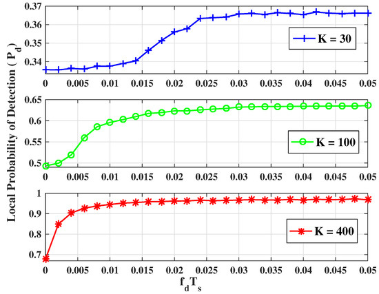
Figure 4. The detection probability of local sensing for various $f_d{T}_s$ (N = 1, ${\eta }_0$ = −8 dB, ${\overline{P}}_f$ = 0.1).

The deterioration in the performance for a reasonably high correlation can be compensated by using a larger number of samples. Next, let us define the minimum number of samples, $K^{*}$, which could be designed and evaluated so as to satisfy any given detecting requirement as

$$\begin{array}{c}\hfill K^{*}\stackrel{\Delta }{=}arg\underset{K}{min}\left\{K:{\overline{P}}_f\le {\xi }_1,{\overline{P}}_d\ge {\xi }_2\right\}\end{array}$$

(44)

In Figure 5, we plot the minimum number of sampling observations required to obtain the desired values (${\xi }_1=0.1,{\xi }_2=0.9$). It is clear that the required number of sampling observations increased dramatically when the normalized Doppler shift, $f_d{T}_s$, is smaller.

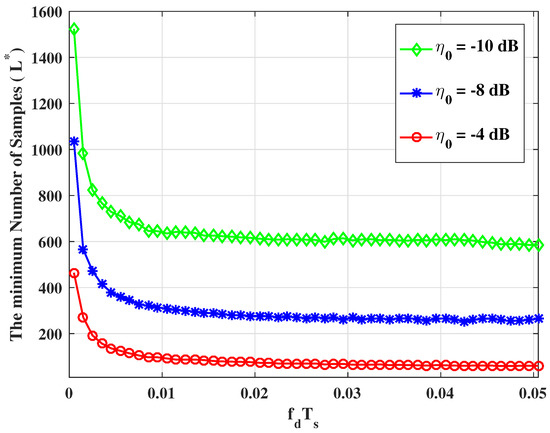
Figure 5. The minimum number of sampling observations required to come up to an expected detecting performance for local sensing ($N=1$, ${\xi }_1=0.1$, ${\xi }_2=0.9$).

The performance of any spectrum sensing technology is dependent evidently on the SNR of detective signal. In Figure 6, we present the complementary receiver operating characteristic (ROC) curves for various average SNR. As shown, the detection accuracy of energy detector can be consistently enhanced by increasing the SNR. With the SNR increasing, the gap of the detection performance between ${\mathcal{C}}_3$ and ${\mathcal{C}}_1$ has become wider. Meanwhile, the theoretical results here compared with the simulating results for both ${\mathcal{C}}_1$ and ${\mathcal{C}}_3$, so that the effectiveness of the analysis is justified (relative error less than $5\%$). The figure indicates that the expression (19) and (12), (20) give the lower and upper bounds of the detection probability for ED-based spectrum sensing under time-correlated Rayleigh fading channels.

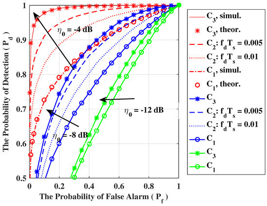
Figure 6. The ROC curves of local sensing for various average SNR ($N=1$, $K=100$).

In the following, we are going to focus attention on cooperative cases. For any cooperation strategy, the number of SVUs participating in the cooperation is of utmost importance. In Figure 7 and Figure 8, the average probability of detection (${\overline{P}}_D$/${\overline{Q}}_D$) are plotted as a function of the number of SVUs for soft fusion and hard fusion strategy, respectively. As expected, the sensing performance shows a upward trend as the number of SVUs increases regardless of fusion strategy. Regarding soft fusion, Figure 7 clearly demonstrate that the theoretical and simulating results also keep in consistent with each other for both ${\mathcal{C}}_1$ and ${\mathcal{C}}_3$, confirming the accuracy of theoretical calculation. Regarding hard fusion, as can be seen from Figure 8, the fit between the theoretical and simulating results may not be very good when the number of SVUs is small but is very accurate for a relatively larger number of SVUs. Similarly, let us define the minimum number of SVUs, $N^{*}$, which could be evaluated so as to satisfy the desired detection requirements as

$$\begin{array}{c}\hfill N^{*}\stackrel{\Delta }{=}arg\underset{N}{min}\left\{N:{\overline{P}}_F\left({\overline{Q}}_F\right)\le {\xi }_1,{\overline{P}}_D\left({\overline{Q}}_D\right)\ge {\xi }_2\right\}\end{array}$$

(45)

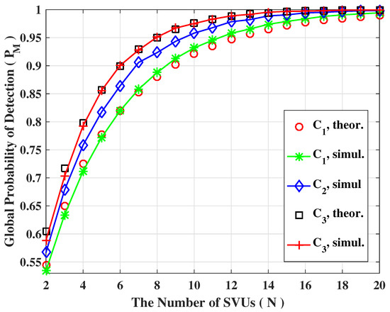
Figure 7. The detection probability of soft fusion scheme for various number of SVUs ($K=50$, ${\eta }_0$ = −8 dB, ${\overline{P}}_F$ = 0.1, ${\mathcal{C}}_2:f_d{T}_s$ = 0.01).

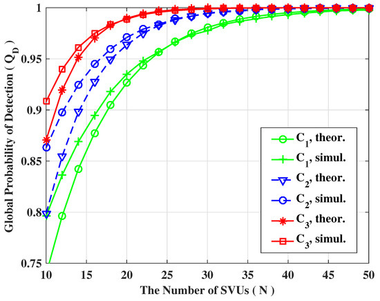
Figure 8. The detection probability of hard fusion scheme for various number of SVUs ($K=50$, ${\eta }_0$ = −8 dB, ${\overline{Q}}_F=0.1$, ${\mathcal{C}}_2:f_d{T}_s=0.01$).

In Figure 9, we plot the minimum number of SVUs required to obtain the desired performance (${\xi }_1=0.05,{\xi }_2=0.95$). It is clear that, as the average SNR decreases, the gap between the required minimum number of SVUs for HF and SF based cooperative sensing is getting further apart, which is because energy detector performed poorly at low average SNR. Moreover, soft fusion has found favor in low traffic, while hard fusion might be preferred in dense traffic.

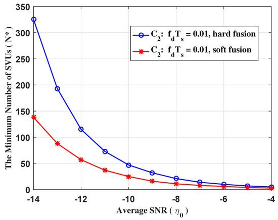
Figure 9. The minimum number of SVUs required to come up to an expected detecting performance for cooperative sensing ($K=50$, ${\xi }_1=0.05$, ${\xi }_2=0.95$).

Besides, we demonstrate the comparison for the performance of soft fusion and hard fusion based cooperative sensing, and present the corresponding results in Figure 10 and Figure 11. It can also be seen clearly that, although soft fusion imposes a large control overhead, soft fusion is always more competitive than hard fusion.

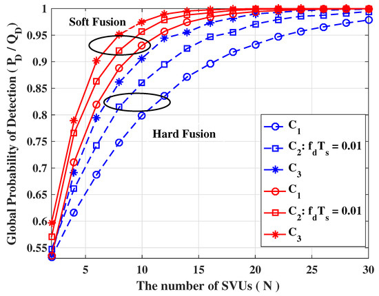
Figure 10. The detection probability of cooperative sensing for various number of SVUs ($K=50$, ${\eta }_0$ = −8 dB, ${\overline{P}}_F/{\overline{Q}}_F=0.1$).

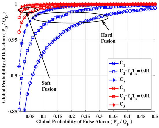
Figure 11. The ROC curves of cooperative sensing ($N=20$, $K=50$, ${\eta }_0$ = −8 dB).

5. Conclusions and Future Work

This paper contains a theoretical and simulated discussion of the performance of spectrum sensing in time-correlated Rayleigh vehicular environments. To study the effect of correlation on detecting performance we considered three models. The probability of detection expressions are given for the special cases. The results obtained reveal the detection performance exasperates with the increasing correlation among the samples. Therefore, it is clearly shown that the effect of correlation cannot be neglected in cognitive vehicular environments operating in a time-correlated case. In our future work, we will continue our efforts to propose a novel soft-hard combination scheme for cooperative spectrum sensing in an inhomogeneous CVN. According to its own conditions, the SVU transmits its hard-decision or soft-data to the FC. Based on the received hard-decision and soft-data, the FC employs a hybrid fusion scheme to make a global decision on the status of the PU. The soft-hard combination scheme aims at taking the best of the two previously fusion scheme (SF and HF) while avoiding the respective disadvantages. As an element task, the current work plays a helpful role in designing a novel soft-hard fusion methods to combat the channel correlation effects for an optimal CVN.

References

- Karagiannis, G.; Altintas, O.; Ekici, E.; Heijenk, G.; Jarupan, B.; Lin, K.; Weil, T. Vehicular networking: A survey and tutorial on requirements, architectures, challenges, standards and solutions. IEEE Commun. Surv. Tutor. 2011, 13, 584–616. [Google Scholar] [CrossRef]
- Haykin, S. Cognitive radio: Brain-empowered wireless communications. IEEE J. Sel. Areas Commun. 2005, 23, 201–220. [Google Scholar] [CrossRef]
- Singh, K.D.; Rawat, P.; Bonnin, J. Cognitive radio for vehicular ad hoc networks (CR-VANETs): Approaches and challenges. EURASIP J. Wirel. Commun. Netw. 2014, 2014, 49. [Google Scholar] [CrossRef]
- Ali, A.; Hamouda, W. Advances on spectrum sensing for cognitive radio networks: Theory and applications. IEEE Commun. Surv. Tutor. 2017, 19, 1277–1304. [Google Scholar] [CrossRef]
- Awin, F.; Abdel-Raheem, E.; Tepe, K. Blind spectrum sensing approaches for interweaved cognitive radio system: A tutorial and short course. IEEE Commun. Surv. Tutor. 2019, 21, 238–259. [Google Scholar] [CrossRef]
- Arjoune, Y.; Kaabouch, N. A comprehensive survey on spectrum sensing in cognitive radio networks: Recent advances, new challenges, and future research directions. Sensors 2019, 19, 126. [Google Scholar] [CrossRef] [PubMed]
- Akyildiz, I.; Lo, B.; Balakrishnan, R. Cooperative spectrum sensing in cognitive radio networks: A survey. Phys. Commun. 2011, 4, 40–62. [Google Scholar] [CrossRef]
- Cichon, K.; Kliks, A.; Bogucka, H. Energy-efficient cooperative spectrum sensing: A survey. IEEE Commun. Surv. Tutor. 2016, 18, 1861–1886. [Google Scholar] [CrossRef]
- Kremo, H.; Altintas, O. On detecting spectrum opportunities for cognitive vehicular networks in the TV white space. J. Sign. Process. Syst. 2013, 73, 243–254. [Google Scholar] [CrossRef]
- Min, A.W.; Shin, K.G. Impact of mobility on spectrum sensing in cognitive radio networks. In Proceedings of the ACM Workshop on Cognitive Radio Network (CoRoNet), Beijing, China, 21 September 2009; pp. 13–18. [Google Scholar]
- Gao, N.; Jing, X.; Huang, H.; Mu, J. Robust collaborative spectrum sensing using PHY-layer fingerprints in mobile cognitive radio networks. IEEE Commun. Lett. 2017, 21, 1063–1066. [Google Scholar] [CrossRef]
- Wang, X.Y.; Ho, P.H. A novel sensing coordination framework for CR-VANETs. IEEE Trans. Veh. Technol. 2010, 59, 1936–1948. [Google Scholar] [CrossRef]
- Xu, Y.; Cheng, P.; Chen, Z.; Li, Y.; Vucetic, B. Mobile collaborative spectrum sensing for heterogeneous networks: A bayesian machine learning approach. IEEE Trans. Signal Process. 2018, 66, 5634–5647. [Google Scholar] [CrossRef]
- Salahdine, F.; Ghribi, E.; Kaabouch, N. A cooperative spectrum sensing scheme based on compressive sensing for cognitive radio networks. Int. J. Digit. Inf. Wirel. Commun. (IJDIWC) 2019, 9, 124–136. [Google Scholar]
- Aygun, B.; Wyglinski, A.M. A voting based distributed cooperative spectrum sensing strategy for connected vehicles. IEEE Trans. Veh. Technol. 2017, 66, 5109–5121. [Google Scholar] [CrossRef]
- Hill, E.; Sun, H. Double threshold spectrum sensing methods in spectrum-scarce vehicular communications. IEEE Trans. Ind. Inform. 2018, 14, 4072–4080. [Google Scholar] [CrossRef]
- Paul, A.; Kunarapu, P.; Banerjee, A.; Maity, S. Spectrum sensing in cognitive vehicular networks for uniform mobility model. IET Commun. 2019, 9, 1–17. [Google Scholar] [CrossRef]
- Bera, D.; Chakrabarti, I.; Pathak, S.S.; Karagiannidis, G.K. Another look in the analysis of cooperative spectrum sensing over nakagami-m fading channels. IEEE Trans. Wirel. Commun. 2017, 16, 856–871. [Google Scholar] [CrossRef]
- Souid, I.; Chikha, H.B.; Attia, R. Blind spectrum sensing in cognitive vehicular ad hoc networks over Nakagami-m fading channels. In Proceedings of the IEEE International Conference on Electrical Sciences and Technologies in Maghreb (CISTEM), Tunis, Tunisia, 3–6 November 2014; pp. 1–5. [Google Scholar]
- Balam, S.K.; Siddaiah, P.; Nallagonda, S. Performance analysis of decision/data fusion-aided cooperative cognitive radio network over generalized fading channel. IEEE Trans. Aerosp. Electr. Syst. 2019, 55, 2269–2276. [Google Scholar] [CrossRef]
- Nallagonda, S.; Kumar, G.K.; Nallagonda, A.K. A comprehensive performance analysis of data-fusion aided cooperative cognitive radio network over η-μ fading channel. IET Commun. 2019, 13, 2558–2566. [Google Scholar] [CrossRef]
- Chembe, C.; Noor, R.M.; Ahmedy, I.; Oche, M.; Kunda, D.; Liu, C.H. Spectrum sensing in cognitive vehicular network: State-of-art, challenges and open issues. Comput. Commun. 2017, 97, 15–30. [Google Scholar] [CrossRef]
- Jakes, W.C. Microwave Mobile Communications; Wiley: New York, NY, USA, 1974. [Google Scholar]
- Gradshteyn, I.; Ryzhik, I. Table of Integrals, Series, and Products; Academic: San Diego, CA, USA, 2007. [Google Scholar]
- Manesh, M.R.; Apu, M.S.; Kaabouch, N.; Hu, W. Performance evaluation of spectrum sensing techniques for cognitive radio systems. In Proceedings of the 2016 IEEE 7th Annual Ubiquitous Computing, Electronics & Mobile Communication Conference (UEMCON), New York, NY, USA, 20–22 October 2016; pp. 1–7. [Google Scholar]
- Li, B.; Zhao, C.; Sun, M.; Zhou, Z.; Nallanathan, A. Spectrum sensing for cognitive radios in time-variant flat-fading channels: A joint estimation Approach. IEEE Trans. Commun. 2014, 62, 2665–2680. [Google Scholar] [CrossRef]
- Atapattu, S.; Tellambura, C.; Jiang, H. Energy detection based cooperative spectrum sensing in cognitive radio networks. IEEE Trans. Wirel. Commun. 2011, 10, 1232–1241. [Google Scholar] [CrossRef]
- Wonseok, C.; Moon-Gun, S.; Jaeha, A.; Gi-Hong, I. Soft combining for cooperative spectrum sensing over fast-fading channels. IEEE Commun. Lett. 2014, 18, 193–196. [Google Scholar]
- Guo, H.; Reisi, N.; Jiang, W.; Luo, W. Soft combination for cooperative spectrum sensing in fading channels. IEEE Access 2017, 5, 975–986. [Google Scholar] [CrossRef]
- Peh, E.C.Y.; Liang, Y.-C.; Guan, Y.L.; Zeng, Y. Cooperative spectrum sensing in cognitive radio networks with weighted decision fusion schemes. IEEE Trans. Wirel. Commun. 2010, 9, 3838–3847. [Google Scholar] [CrossRef]
- Nardelli, P.H.J.; Ramezanipour, I.; Alves, H. Average error probability in wireless sensor networks with imperfect sensing and communication for different decision rules. IEEE Sens. J. 2016, 16, 3948–3957. [Google Scholar] [CrossRef]
- Bae, S.; So, J.; Kim, H. On optimal cooperative sensing with energy detection in cognitive radio. Sensors 2017, 17, 2111. [Google Scholar]
- Juboori, S.A.; Hussain, S.J.; Fernando, X. Cognitive spectrum sensing with multiple primary users in Rayleigh fading channels. Electronics 2014, 3, 553–563. [Google Scholar] [CrossRef]
- Nuttall, A.H. Some integrals involving the QM function. IEEE Trans. Inf. Theory 1975, 21, 95–96. [Google Scholar] [CrossRef]
- Peebles, P.Z.; Shi, B.E. Probability, Random Variables, and Random Signal Principles; McGraw-Hill: New York, NY, USA, 2001. [Google Scholar]
© 2020 by the authors. Licensee MDPI, Basel, Switzerland. This article is an open access article distributed under the terms and conditions of the Creative Commons Attribution (CC BY) license (http://creativecommons.org/licenses/by/4.0/).