Improved RSSI-Based Data Augmentation Technique for Fingerprint Indoor Localisation

Abstract

Recently, deep-learning-based indoor localisation systems have attracted attention owing to their higher performance compared with traditional indoor localization systems. However, to achieve satisfactory performance, the former systems require large amounts of data to train deep learning models. Since obtaining the data is usually a tedious task, this requirement deters the use of deep learning approaches. To address this problem, we propose an improved data augmentation technique based on received signal strength indication (RSSI) values for fingerprint indoor positioning systems. The technique is implemented using available RSSI values at one reference point, and unlike existing techniques, it mimics the constantly varying RSSI signals. With this technique, the proposed method achieves a test accuracy of 95.26% in the laboratory simulation and 94.59% in a real-time environment, and the average location error is as low as 1.45 and 1.60 m, respectively. The method exhibits higher performance compared with an existing augmentation method. In particular, the data augmentation technique can be applied irrespective of the positioning algorithm used.

1. Introduction

Indoor localisation is essential for mobile systems (smartphones, robots, Internet of Things devices, etc.) at several places such as exhibition halls, shopping malls, and office buildings [1]. Accurate, reliable, and real-time localisation is the basis for automatic navigation and task allocation [2]. In particular, the easy accessibility of the Global Positioning System (GPS) from mobile devices such as smartphones has enabled travellers to move around the world more freely. However, the GPS is sensitive to occlusion and cannot be accessed from indoor environments. Several indoor localisation systems [3,4,5,6] with different sensors have been presented. With the pervasive penetration of wireless local area networks and wireless access equipment [7,8,9,10,11,12], Wi-Fi-based indoor localisation [13] has recently attracted considerable attention. In such localisation systems, the use of fingerprint approaches [14] based on the received signal strength have shown significant advantages. If a series of physical locations are selected in a workspace, the signals received at these locations from the access points (APs) in the vicinity of the locations are defined as the fingerprints for the locations. Furthermore, the locations for their corresponding fingerprints are defined as reference points (RPs). In the training phase for fingerprint positioning, the received signal strength indication (RSSI) values are acquired at the identified RPs. In the positioning phase, the observed RSSI is used to determine the device location based on a fingerprint map. WiFi-based fingerprint approaches require neither AP locations nor angle measurements of the signal receiver, and therefore, they are highly feasible for indoor localisation. However, several key problems in Wi-Fi-based indoor localisation are yet to be solved. First, the Wi-Fi signal strength is relatively susceptible to multipath effects and external interference. In addition, the presence of noise may cause the received signal strength to deviate from its true value, leading to a large location error. Second, higher localisation accuracy requires faster Wi-Fi scanning and intensive CPU computations, which involve higher energy consumption. Third, most indoor localisation systems have a time-consuming calibration process. An extensive site survey for fingerprint map construction is time-consuming and labour-intensive. Moreover, a change in the spatial distribution or Wi-Fi environment increases the site survey cost. Consequently, it is required to reduce deployment effort during the calibration of maps for indoor Wi-Fi localisation systems.

Different machine learning methods are used for WiFi fingerprinting to build localization models like k-Nearest Neighbours (KNN) [15], Random forest [16] and Support Vector Machines (SVM) [17]. However, these methods can suffer from limitations on their ability to fully to learn complex features from the training data. On the other hand, deep learning (DL) has been widely applied in various fields. Therefore, the recent works on WiFi-based indoor localization started to use DL models to estimate nodes’ locations [18,19].

The purpose of an augmentation technique is to increase the number of data according to a given measured training set. In [20], mean and uniform random number (MURn) augmentation was proposed to generate the training dataset for the convolutional neural network (CNN) model, for achieving optimum performance for WiFi-based fingerprint indoor localisation. The augmented data were subsequently used to enhance the robustness and accuracy of indoor localisation. In our previous study [21], we employed the data augmentation techniques and resulted in simulation results with the CNN model for indoor positioning. The CNN model was utilized to compare the performance with other CNN applications such as AlexNet, ResNet, ZFNet, Inception v3, and MobileNet v2, for WiFi-based fingerprint datasets. We performed comprehensive testing of our algorithms with these CNN applications to demonstrate the effectiveness of our proposed CNN model.

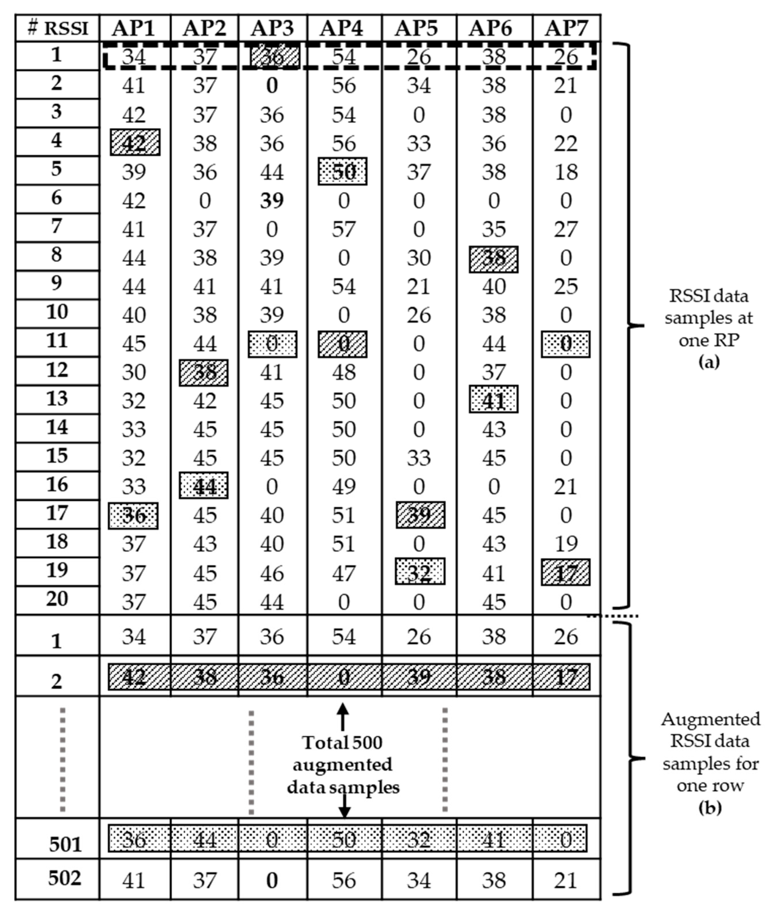
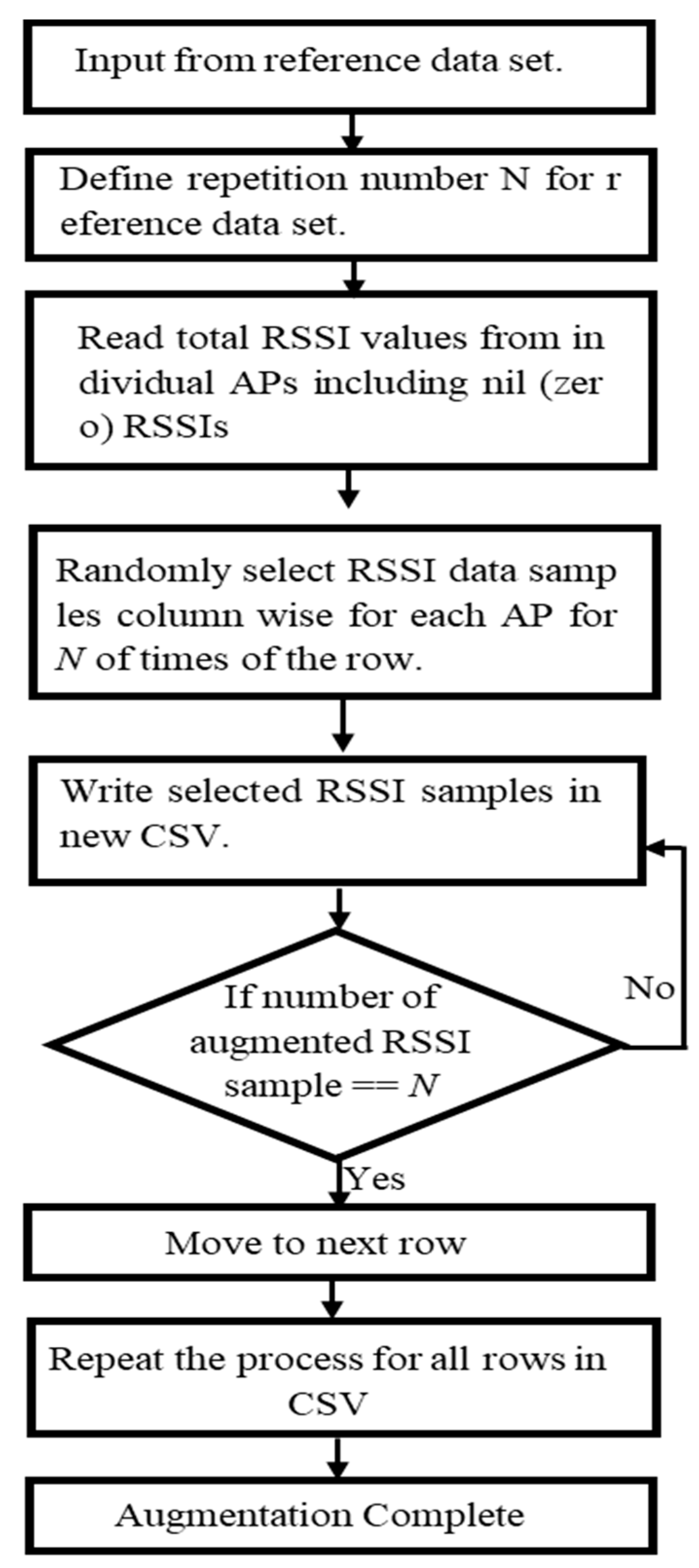
In this study, fingerprint augmentation is conducted for indoor Wi-Fi localisation in order to reduce site survey work and improve the location accuracy in the deployment stage. The RSSI augmentation technique that can be implemented in any deep-learning-based fingerprinting system is proposed. Here, an improved augmentation technique based on RSSI values at APs is introduced. The proposed RSSI-based augmentation is robust, unique and simple to implement, which based on only RSSI values collected at each RP to produce augmented output. The RSSI value present at target RP is randomly selected and written in new output. The robustness lies in the fact that the pattern of augmented output matches with the input RSSI pattern of the target RP. The number of repeated times for random RSSI selection is decided by ‘N’ which is global repetition number. The generated output is based on only target RSSI values for augmentation. Furthermore, we compare the RSSI-based augmentation technique with the MURn augmentation technique with evaluating the performance of the localisation in a six-layer CNN model. The comparison is performed through both laboratory simulation and real-time experiment. The remainder of the paper is structured as follows. Section 2 describes the background work of this study. The proposed RSSI technique is described in Section 3, and a system model and an experimental setup are presented in Section 4. Section 5 compares the numerical results of the RSSI and MURn augmentation techniques. Finally, Section 6 concludes the paper.

2. Background

Figure 1 shows fingerprint indoor localisation systems. Basically, the system operation comprises two states. In the offline stage, the RSSIs for known positions, referred to as RPs, are collected from all APs to construct a fingerprint database for the environment. Therefore, each RP has a fingerprint characterised by its position and the RSSIs captured at the location from all APs in the vicinity. In the positioning stage, the currently captured RSSIs are matched with those of the RPs, and the position is determined from the positions of the best-fitting RPs. In the technique, the data collected by traditional localisation systems are used as the input, and a new larger data set that should be used for training the localisation system is generated; the amount of input data is typically small. In the remainder of this section, we start by describing the hardware and software setup and input data set format and subsequently provide details of the CNN model that we used for position estimation.

All our experiments were conducted on a server with powerful computational capability. The server had 16 GB of memory and was equipped with two GeForce GTX 1080Ti graphics cards to accelerate computing. We installed Windows 10 in conjunction with Python. Python has very efficient libraries for matrix multiplication, which are very useful when working with deep neural networks (DNNs). TensorFlow provides a very efficient framework for implementing the CNN architecture. We also installed dependencies, such as the CUDA Toolkit and CuDNN, before using TensorFlow. The CUDA Toolkit provides a comprehensive development environment for NVIDIA-GPU-accelerated computing, while CuDNN can optimise CUDA to improve its performance.

2.1. Input Data Sets

The data set collected during the measurement was in text format. This text data is converted into a comma-separated values (CSV) file as an input to deep learning code for training and testing purposes. The CSV file contains 257 columns, where column 1 to 256 contains the MAC address of the RP while the 257th column has the RP number from 1 to 74 (Figure 2). The 257th column is the label for deep learning code. The text file is converted to CSV file by a specific conversion code designed by python. The first step of this code is to take input from the folder containing text file. Later, the code reads the RPs and the related MAC addresses. Every new MAC address is given on a column in the CSV file and the corresponding RSSI value is written in the following row. For the other MAC addresses which are not present in the current text file, the RSSI values of zero are entered into the current row. The process continues until all the text files in all the folders are processed. If the total number of columns in the final CSV file is lower than 256, then the remaining columns are filled with zeros. If the total number of columns is greater than 256, then the extra columns are deleted on the basis of minimum RSSI entries for individual MAC addresses. If the total number of columns in the final CSV file is equal to 256, then the reference data set is complete. Figure 2 shows the CSV format for the input file; NN represents an RSSI value.

For our CNN model, a six-layer network was designed to predict 74 classes. The input image was generated from RSSI values received at 74 RPs during the experiment. At each RP, the RSSI value was recorded for 256 APs, although only a small subset of these APs was visible. These RSSI values from different APs were used to generate a 16 × 16 image. In the example in Figure 3, there are nine visible APs out of 256 with RSSI values between 25 and 70, and the RSSI values of the other APs are 0. The RSSI values from different APs were converted into a greyscale image, and the image brightness depended on the recorded RSSI values, with higher RSSI values generating a brighter image. In Figure 3a, the highest RSSI value is 70, and it produced the brightest spot in the greyscale image in Figure 3b; by contrast, the lowest value (25) corresponds to the darkest non-black spot. RSSI values of 0 produce no brightness, and therefore, the remaining 247 spots are black. Similarly, the input RSSI files for the other 73 RPs produce different images when input into the DL network.

2.2. CNN Model

A deep learning architecture is useful for audio, video and image data types. For a CNN, the output from one layer is the input for the subsequent layer. In the CNN, each neuron is interconnected, and it has weight associated to each neuron in the following layer. As a result, the number of required connections in this type of network rapidly grows as the input size increases to an unmanageable level. For example, in [22], if the input to the CNN network is through a VGA camera (640 × 480 × 3 pixels), there would be a weight difference of 921,600 between an input neuron and a single hidden neuron. In addition, the first hidden layer needs to comprise of thousands of neurons to manage the dimensionality of the input, leading to a model with billions of weight values, all of which would need to be learned. It is very difficult to work with this many weight values since it increases the computation complexity as well as the memory requirements. A significant advantage of this method compared with conventional approaches, especially for pattern recognition, is its ability to reduce the dimensions of the data, extract features sequentially, and classify the image at the output of CNN network [23]. Figure 4 presents the architecture of the CNN in this study. We trained the data on a CNN network with different convolutional layers to find the best architecture. In each architecture, we adjusted the filter size, number of feature maps, pooling size, learning rate and batch size in the hyperparameter tuning process to retain the best configuration. We chose the best suited parameter-setting as the final configuration. The list of hyperparameters and their candidate values can be found in our previous work [21]. The best outcome CNN architecture used in our work is as follows-CNN network comprises six layers with first four convolutional layer and two fully connected layer, the first consisting of input 16 × 16 × 1 greyscale images along with a rectified linear unit (ReLU) and dropout. Owing to the input data set’s small size, the first layer does not use max pooling. The second layer consists of a 16 × 16 convolution with an ReLU and an 8 × 8 max pooling layer with 18,496 parameters, and its output is the input of the third 8 x 8 convolution layer (with an ReLU and an 8 × 8 max pooling layer). This output of the third layer is fed to the fourth layer, which is an 8 × 8 convolution layer with an ReLU and an 8 × 8 max pooling layer. This output of the fourth layer is directly fed to a fully connected (FC) layer with 2176 nodes, which leads to another hidden FC layer with 1088 nodes. Finally, the output is calculated using a softmax layer with 74 nodes, which is equal to the total number of RPs in our setup. The inner width is 128, and while the first three layers have no dropout, the fourth layer has a dropout of 0.5. The learning rate of our CNN model is 0.001, and the total number of parameters is 233,418 [21].

3. Proposed Augmentation Technique

3.1. RSSI Samples

The RSSI measured by smartphones contains complex noise, which seriously affects the positioning accuracy. Furthermore, it is difficult for a Wi-Fi system to transmit signals with a fixed power, which results in time-varying characteristics of the RSSI. Moreover, indoor electromagnetic environments are complex and are characterised by multipath fading and other noise. We examined the RSSI fluctuation for five different APs by considering 20 RSSI samples; the fluctuations are shown in Figure 5. These RSSI samples have been acquired in the same way as the training data set. i.e., the device is set on a target RP and 20 RSSI sample values are collected. Clearly, owing to the instability of the Wi-Fi system, the RSSI values were time-varying, with the maximum fluctuation value being about 37 units for AP 1, 40 units for AP 2, 44 units for AP 3, 50 units for AP 4 and 39 units for AP 5. Figure 5 confirms the unstable nature of the RSSI signals transmitted by the Wi-Fi AP. The maximum fluctuation for each AP confirms that the variation of the RSSI signals is uncertain. This characteristic of the RSSI signals affected the overall test accuracy of the DL system and resulted in erroneous predictions of locations. At an RP, approximately 130 RSSI data samples obtained from 256 APs can be used to generate RSSI with a variation and uncertainty characteristic of the APs at the location. These generated RSSI data samples are called augmented RSSI data samples, and they mimic the original RSSI values. Hence, they can be used to train the CNN model for position estimation.

3.2. Proposed RSSI-Based Augmentation Technique

In a fingerprinting algorithm, the fingerprint of each training point is a sequence of measurements from different APs; the numbers of measurements from any two APs are identical. Therefore, for M measurements per RP and A APs, the fingerprint at each RP has the dimensions A × M. The objective of the algorithm is to classify a test point as one of those RPs by using CNN classifiers. However, if only a few observations are available for a given class, the CNN will not be able to gather sufficient information for a particular location. Therefore, multiple observations are required for each class. To increase the training data set to an appropriate size, augmentation is employed. The RSSI-based augmentation deals with the collected RSSI data sets at 74 RPs. If the data set has ‘X’ RSSI value at each RP, then for each RSSI reading, it randomly selects ‘N’ number of RSSI values at the RP. Therefore, total number of RSSI values at one RP will be (X × N) + 1. These randomly selected RSSI values are written in separate CSV file. Note that by using the collected RSSI values at each RP, this augmentation can not only increase the number of RSSI signals for the DL classifier but it also successfully retains the pattern of the collected RSSI values at the RP. Figure 6 shows the patterns of RSSI and augmented RSSI data at an RP for 100 RSSI data samples obtained from one AP (dotted red curve). The solid green curve connects 100 augmented RSSI data for the same AP at the same RP, and it mimics the curve connecting the original RSSI samples. The trend lines (straight lines), also known as ‘best-fit lines’, indicate the overall data pattern trend of both RSSI and augmented RSSI data samples. The dotted straight line shows the trend of the RSSI data samples, and the solid straight line indicates the trend of the augmented RSSI data samples. The overall patterns of the two trend lines are similar. This shows the similarity in data variation over a period of time and the correlation of a variable before and after augmentation.

The further technical detail of RSSI augmentation are as follows. In the augmentation technique, the data are augmented on the basis of previously collected RSSI data samples from each RP. As discussed in Section 2, an input RSSI sample with 256 values generates a 16 × 16 greyscale image. Therefore, each row of the input CSV file containing RSSI data samples contributes to one training input image for the CNN model. Figure 7 shows 130 RSSI data samples for seven of the 256 APs (Figure 7a). The global repetition number N is declared, and the input data set is obtained in the form of CSV files. The first row of the figure (red dotted box) contains the first RSSI data samples for data augmentation. For AP 1, the complete column with 130 RSSI data samples is selected. With the help of the Python function ‘enumerator’, the initial counter is set for AP 1 to AP 7, and it selects one RSSI value out of the 130 RSSI data samples. In Figure 7a, row 1 (dashed-line box) value is selected and written in the CSV file, the counter’s count increases by one for all 256 APs. Figure 7b row 2 shows the selected RSSI data samples with diagonal-lined box. In Figure 7a diagonal-lined box represents the first augmented RSSI data sample row, while the dotted-lined box represents the last augmented RSSI data sample row. In this work, the optimum value of N was selected as 500. Therefore, this process was repeated until the number of rows for the selected input row equalled 500. The first row of the augmented RSSI data is the same row as that of the input CSV file. The total number of rows for one input row is N + 1. In Figure 7b, the first row is the same as the red dotted row of Figure 7a, and the index count of the augmented rows increases up to N + 1, that is, row 501 for the given input CSV file. From row 502 (Figure 7b), the RSSI augmentation process is repeated same as row 1 of Figure 7a. The pseudocode scheme (Algorithm 1) and flow graph (Figure 8) explain the coding for the RSSI augmentation technique in considerable detail. There were a total of 65,130 augmented image files for one RP and a total of about 4,819,620 images for 74 RPs.

Algorithm 1: Pseudocode for RSSI augmentation technique

Define ‘N’ DefineHeader for input CSV file       for total number of reference points (RPs)             for each AP address per RP                    if current RSSI ≠ 0                         Read total of the RSSI values for the current RP                                 Randomly select N RSSI from current RP.                                 if current RSSI value == 0                                     Repeat zero value RSSI == N times                                 end if                            Repeat the process for all the RSSI values for the current RP                         end if              end for        end for  end for

4. System Model and Experimental Setup

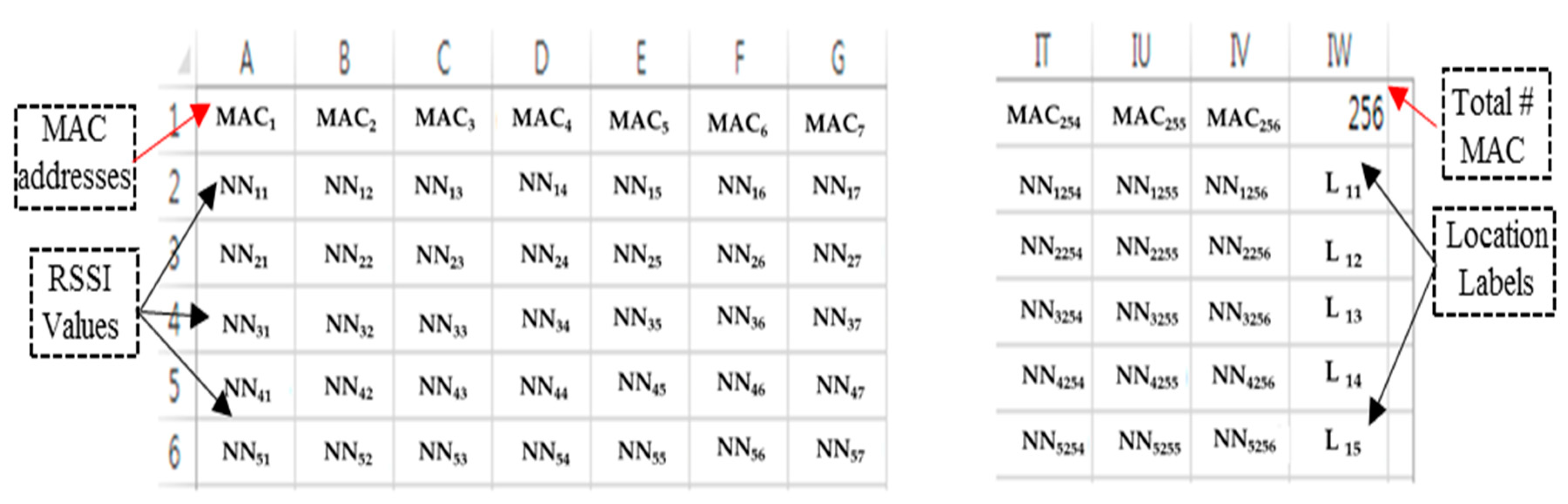
The CSV files used in this study contained 257 columns and 74 RPs in the 257th column; the RPs served as labels. Data conversion was performed using Python. The input for the file converter code (written in Python) comprised folders containing text files. To assess the validity of our approach, we collected seven data sets over a week, which were then used to assess the CNN layer that was best suited to transfer knowledge from classification to indoor positioning as well as to identify the optimal classification algorithm. The results showed that a relatively simple classification model fitted the data well, producing about 95% generalisation over a one-week period in laboratory-based simulations with RSSI augmentation. It was necessary to train the classification model with data reflecting the effect of the introduction of new APs’ and changes in the existing APs. To generate the data set, the data were collected over seven days in four directions namely forward, backward, left and right at the 74 RPs to reflect the dynamic environment on training data set. As summarized in

Table 1. Data set collection.

Training Data Set Collection
Days	Morning/Afternoon		Afternoon/Evening
	09:30 am. to 11:30 am.	12:00 pm. to 02:00 pm.	2:30 pm. to 04:30 pm.	05:00 pm. to 07:00 pm.
Day-1	Forward	Left	Right	Backward
Day-2	Left	Right	Backward	Forward
Day-3	Right	Backward	Forward	Left
Day-4	Backward	Forward	Left	Right
Day-5	Forward	Left	Right	Backward
Day-6	Left	Right	Backward	Forward
Day-7	Right	Backward	Forward	Left
Real time testing
Day-1	Forward		Backward
Day-2	Backward		Forward
Day-3	Forward		Backward
Day-4	Backward		Forward
Day-5	Forward		Backward

, the training data set was collected over two time periods, namely, Morning/Afternoon and Afternoon/Evening to reflect the human activities. The Morning/Afternoon includes 09:30 to 11:30, a highly active period and 12:00 to 14:00, a moderately active period. The Afternoon/Evening covers low to high active time from 14:30 to 16:30 and 17:00 to 19:00. Also, the orientation of the device is kept in four directions to reflect the diversity in the training data set, which considered the diversity of the RSSI values from the surrounding APs with the different directions. Using this training with such data set, the CNN classifier may correctly predict the use position for online experiment, even if the user moves in a slightly or fully left- or right-oriented way. In the real time testing, the movement of people went forward and backward, which was done for five days.

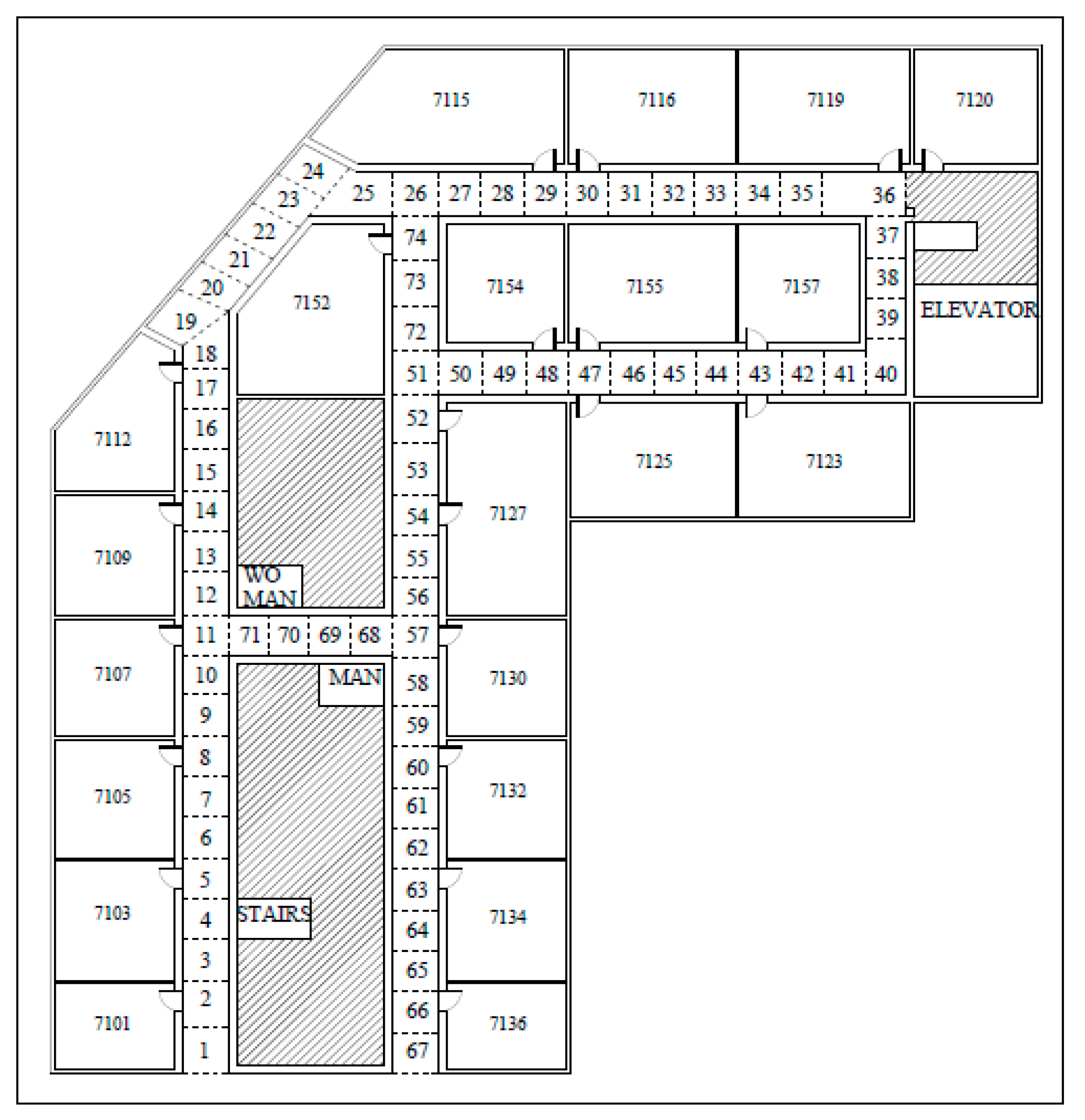
RSSI fingerprint data collection and the final experiment were both performed on the 7th floor of the new engineering building at Dongguk University, Seoul, Korea. As shown in Figure 9, the 52 × 32 m target area with the roof height of 3 m is divided into 74 target RPs. The RPs such as 1, 25, 36, 40 and 67 are at the corner and their sizes vary between 2 m to 3 m, i.e., +1 m difference. Meanwhile, the RPs such as 10, 11, 18, 50, and 71 are at the ending spot and their sizes vary between 1 m to 2 m, i.e., −1 m difference. Note that the RP block size is approximately 2 m × 2 m while ranging from 1 m to 3 m for specific locations. The positioning server used in this study is a Dell Alienware Model P31E (Alienware, hardware subsidiary of Dell, Miami, FL, USA), and the smartphone for data collection is a Samsung SHV-E310K (chip fabrication Yongin-si, Gyeonggi-do, Korea). The fingerprint database construction, classification (i.e., position prediction), and online experimental setup are developed with Python.

The data read by an Android device were stored in a buffer. If there was an error in the recorded data, an error message was displayed on a serially connected console. Otherwise, the RSSI data were stored in the buffer, and after a complete scan, they were transferred by the Android console, which was connected by an interface cable to the server, to the server through a Wi-Fi AP. The server determines the Android device’s location by comparing the measured RSSI values with reference data. It was serially connected to the Android console and processed the RSSIs obtained from the surrounding APs with its CPU. The operating frequency of the device was 2.412–2.480 GHz for the 802.11bgn wireless standard. The input/output sensitivity was 15–93 dBm.

5. Numerical Results

We compared our RSSI augmentation technique with MURn augmentation. As mentioned in the previous section, the RSSI data samples were collected over seven days. The total number of RSSI data samples for one RP was approximately 130. These RSSI data samples were used as the input image for the augmentation. Few RPs had only 128 or 129 samples since the collected RSSI sample text file sometimes contained no data and was therefore deleted from the data set. The global value of RSSI augmentation was 500, and the total number of images for one RP was about 65,130. A total of 4,819,620 CNN training images were used for the RSSI-based augmentation technique and 596,440 CNN training images were employed for MURn augmentation. The total number of images used for the MURn augmentation technique for the 130 input image files was about 8060. The total number of test images for the laboratory simulations is 1479. The laboratory simulation is a process where the augmented data set is used to train the CNN classifier and the remaining data set is tested by the trained CNN classifier. Meanwhile, real time testing is a process where, with the trained CNN classifier, the user’s position is predicted by using the RSSI dataset received from the APs.

The global repetition number is important when choosing an augmentation technique.

Table 2. Effect of global repetition number on augmentation techniques.

Global Repetition Number N	Data Set Size (Kilobyte)		Training Accuracy (%)		Test Accuracy (%)
	RSSI-Based Aug.	MURn Aug.	RSSI-Based Aug.	MURn Aug.	RSSI-Based Aug.	MURn Aug.
60	301,679	326,658	63.10	86.99	93.80	94.11
100	495,128	500,503	63.46	83.37	95.06	93.78
150	985,013	746,861	62.26	87.97	94.99	93.78
200	1,008,954	994,166	61.96	83.95	95.06	93.78
500	2,455,849	2,247,999	63.26	95.39	95.26	89.04
1000	4,906,760	4,951,046	63.46	96.23	94.79	88.95

shows the impact of N with six different values on the augmentation technique. The value of N determines whether the training of the CNN model is optimised, since it can help the CNN model to learn more efficiently. The training accuracy can be defined in the terms of loss value, which tells how well the CNN classifier learns from the training images to predict the test image correctly for each reference point. The test accuracy indicates how many test data are identified correctly. A higher test accuracy is desirable in accuracy of positioning case since it reflects least error between training and testing environments. With N = 60, the training accuracy of the CNN model is 63.10% for RSSI-based augmentation and 86.99% for MURn augmentation, and the test accuracy is 93.80% and 94.11%, respectively. Similarly, at N = 200 the training accuracy is 61.92% and 83.95% and the test accuracy is 95.06% and 93.78%, respectively. For N = 500, the training accuracy is 63.26% and the test accuracy is 95.26% which is the highest for the RSSI-based augmentation. Meanwhile, the test accuracy for MURn augmentation is as low as 89.04%. Therefore, the RSSI-based augmentation gives an advantage in test accuracy since increasing the data set size can retain the characteristics of the RSSI values for the augmentation.

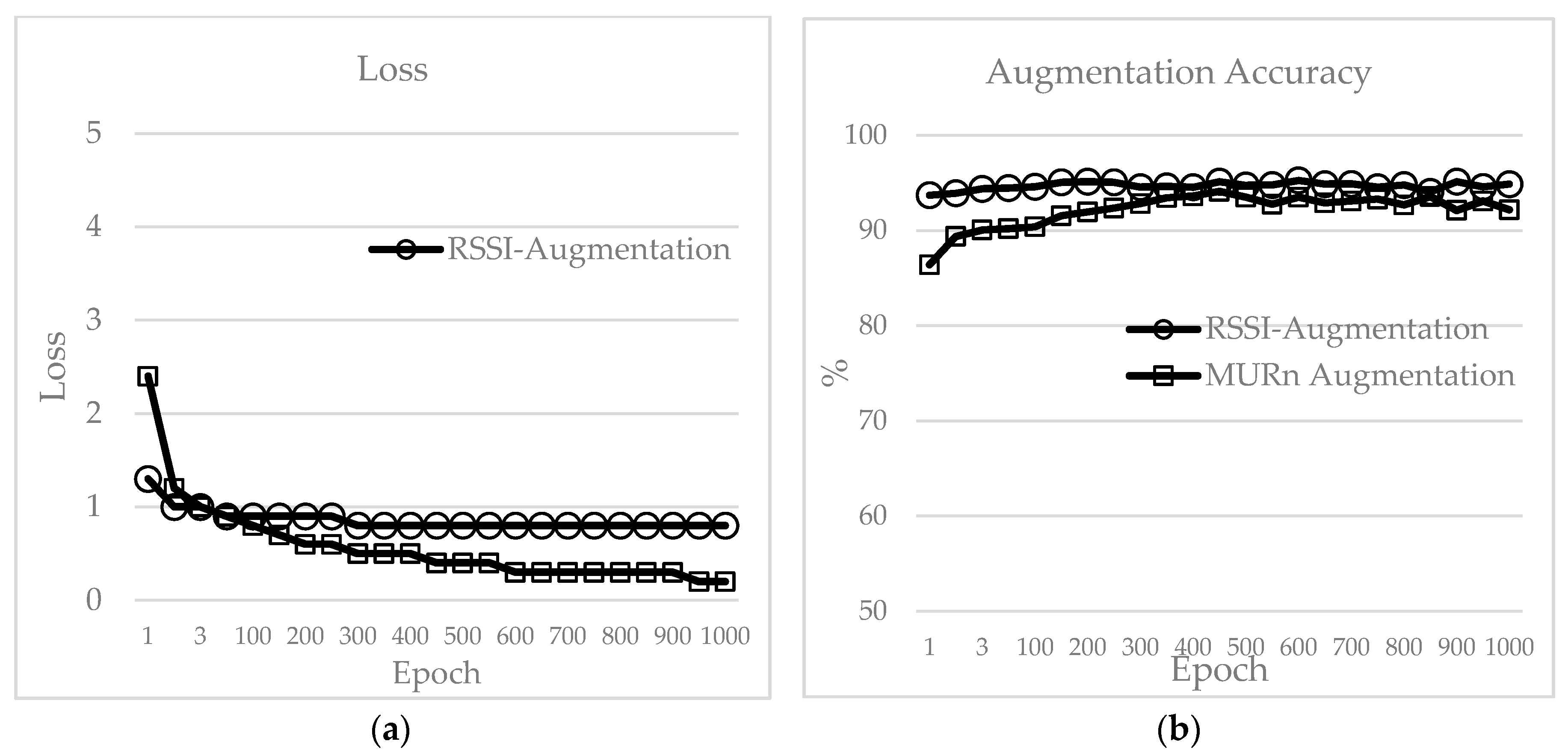
Figure 10a,b shows the laboratory simulation results for the loss and test accuracy of the RSSI augmentation and MURn augmentation techniques. The loss values for RSSI and MURn augmentation start at 1.3 and 2.4, respectively, and they reach to 0.8 and 0.4, at epoch 500, respectively. The loss value after epoch 1000 remains at 0.8 for the RSSI augmentation technique, while for MURn augmentation, the loss reduces to 0.2. The loss decreases after epoch 1000 for MURn, and this shows the robustness of the training data and CNN model. However, the accuracy of the model also decreases, which is undesirable for indoor positioning. The highest accuracy achieved in the laboratory simulations for each of the techniques was used as the optimum value to generate the metafile [7] for the real-time testing of the techniques. Therefore, the highest accuracies were chosen for the RSSI augmentation and MURn augmentation data sets in this study. The highest accuracy for the RSSI augmentation data set was 95.26%, and it was achieved after epoch 643; the loss value was 0.8. For the MURn augmentation technique, the highest accuracy chosen was 94.44% at epoch 450, and the loss at this point was 0.4. After epoch 1000, the test accuracy of RSSI augmentation remained constant at about 94% (loss: 0.8), while the MURn augmentation accuracy decreased to about 92% (loss: 0.2).

Table 3. Laboratory simulation results for training CNN models with augmented data sets.

Augmentation	Epoch Time (Minute)	Loss	Training Accuracy	Test Accuracy
RSSI-based Augmentation	2.50	0.8	63.26	95.26
MURn Augmentation [21]	0.13	0.4	86.99	94.44

summarises the CNN model performance for both augmentation techniques. The longer epoch time of RSSI augmentation compared to that of MURn augmentation was because of the effect of N (Table 3). Each collected RSSI sample was repeated N (=500) times, and therefore, the overall data set size increased to 2 GB, thereby increasing the epoch time. Thus, there is a trade-off between the test accuracy and the epoch time in the RSSI augmentation technique.

The number of RPs predicted accurately in the real-time experiment by the CNN model trained with augmented RSSI data sets was called the zero-margin accuracy, i.e., zero meter error. When the predicted test RP matches with neighbouring RP it is called one margin accuracy, i.e., 2 m error. Similarly, when the test RP matches with difference of two RP it is known as two margin accuracy, i.e., 4 m error. A comparison of the real-time prediction accuracies of the CNN mode for different margins and for the two techniques is presented in

Table 4. Real-time accuracy comparison for zero, one and two margins for CNN models trained with augmented RSSI data sets.

Augmentation	Zero Margin	One Margin	Two Margins
RSSI-based Augmentation	43.78	83.24	94.59
MURn Augmentation	37.30	75.40	92.44

. The model had the highest zero-margin accuracy, 43.78%, for RSSI augmentation, while for MURn augmentation, the zero-margin accuracy was 37.30%, which is lower than that for RSSI augmentation by 6.48%. A two-meter difference between the actual and predicted RP was termed one-margin accuracy. For RSSI augmentation and MURn augmentation, the one-margin accuracy was 83.24% and 75.40%, respectively, is the difference being 7.84%. A difference of four meters between the predicted and actual outputs was called two-margin accuracy. The highest two-margin accuracy for RSSI and MURn augmentation was 94.54% and 92.44%, respectively. Thus, the two-margin accuracy difference between both augmentation techniques was only 2.15%.

An indoor localisation system is best evaluated on the basis of performance statistics by using the mean value, variations, and standard deviation. The mean is the average value of all distance errors in terms of metres for indoor localisation, which is desirable to be as close to zero as possible.

Table 5. Performance statistics of CNN trained on RSSI data sets.

Augmentation	Mean (m)		Variation (m)		Standard Deviation (m)
	Real Time	Lab Simulation	Real Time	Lab Simulation	Real Time	Lab Simulation
RSSI-based Augmentation	1.60	1.45	3.33	3.22	1.83	1.79
MURn Augmentation	2.06	1.48 [21]	5.96	5.54 [21]	2.44	2.38 [21]

shows a comparison of the performance of both augmentation techniques in the laboratory simulation as well as real-time experiment. RSSI augmentation achieved mean errors as low as 1.60 m in the real-time experiment, which is close to the laboratory simulation mean error of 1.45 m. The MURn augmentation mean error was 2.06 m in the real-time experiment and 1.48 m in the laboratory simulation. The mean errors of the two augmentation techniques in the laboratory simulation were very close, while they varied by 0.5 m in the real-time experiment. This variation is continued to be observed in real time and lab simulation for both augmentation results. The RSSI augmentation variation was 3.33 m in the experiment and 3.22 m in the simulation. The variation for MURn augmentation was 5.96 m in the experiment and 5.54 m in the simulation, which was about 2 m higher compared with that for the RSSI augmentation technique. The standard deviation for RSSI augmentation was 1.83 m in the experiment and 1.79 m in the simulation; the values are close to each other. The standard deviations for MURn augmentation in the experiment and simulation were 2.44 and 2.38 m, respectively. The performance in the lab simulation matches with that in the real-time experiment for both augmentation techniques. The RSSI augmentation technique’s performance was better that the MURn augmentation technique’s performance.

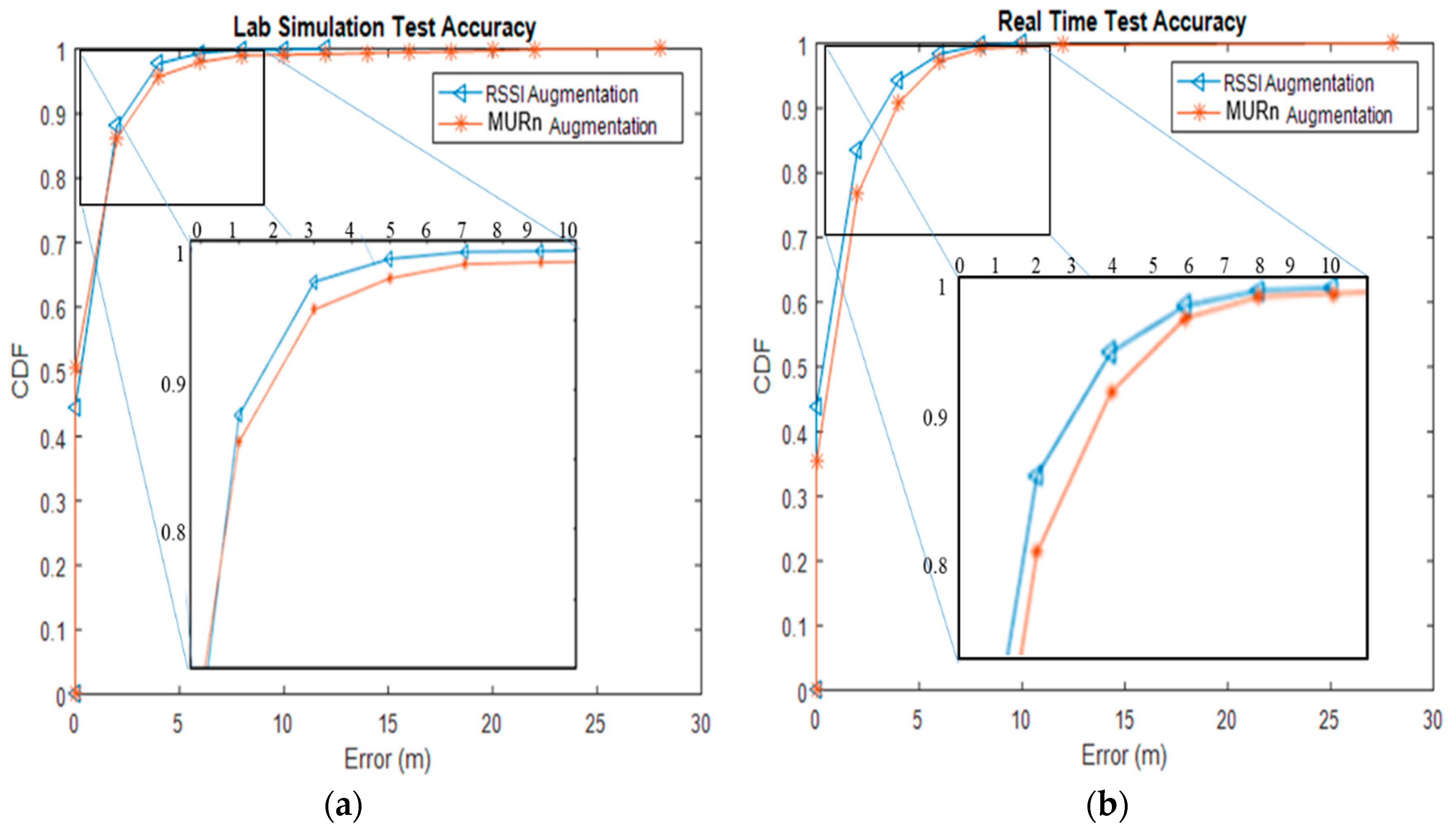
We also evaluated the effectiveness of indoor positioning (i.e., positioning accuracy), defined as the cumulative percentage of the location error within a specified distance (Figure 11). This was evaluated in real time as well as in the laboratory simulation. In the laboratory simulation, the test accuracy of the RSSI augmentation technique did not differ significantly with a change in the positioning accuracy (e.g., cases where the error distance was within 5 m). The probability of being within an error distance of 5 m was above 90% for both augmentation techniques. However, for cumulative distribution functions over 90%, the positioning accuracy of MURn augmentation falls below that of the RSSI augmentation technique. Under 90%, the error distance for the augmentation techniques in the laboratory simulation was about 2.5 m, with RSSI augmentation being more accurate than MURn augmentation by around 0.50 m. The performance gap between the two techniques increased gradually, and eventually the error distance increased to nearly 10 m for RSSI augmentation and 28 m for MURn augmentation. The real-time position accuracies for both augmentation techniques are shown in Figure 11b. The error distance of the RSSI augmentation technique was lower than that of the MURn augmentation technique in the range 0–10 m. Under 90%, the error distance for both augmentation techniques in the real-time simulation was about 2.5 m, with the RSSI augmentation technique being more accurate by around 0.50 m. The performance gap between the two techniques increased gradually, and eventually the error distance increased to nearly 10 m for the RSSI augmentation technique and 28 m for MURn augmentation.

The average test accuracies for both augmentation techniques were compared for a real environment. The environmental conditions were the same for all five days of the test. The RSSI augmentation technique showed the highest accuracy of 94.53% for Day 5 and the lowest test accuracy of 86.36% for Day 2. MURn augmentation showed the highest accuracy of 92.44% for Day 1 and the lowest accuracy of 87.03% for Day 4. Overall, the RSSI augmentation technique performed better. For example, this technique had a mean error of 1.60 m when an augmented training data set with data for seven days was used to assist in localisation, while MURn had a mean error of 2.06 m. In other words, the RSSI augmentation technique performed better than MURn augmentation by 2.65%. Furthermore, the performance of the former in terms of accuracy was very close to the lower error bound, for which the median error was 1.45 m.

6. Conclusions

In this paper, an efficient data augmentation technique for DL-based indoor positioning is proposed. We propose an RSSI augmentation technique that can generate augmented RSSI data that mimic the original RSSI samples and that can be integrated with any fingerprinting-based DL technique to increase the training data set by varying the global repetition number N. A four-layer CNN structure was trained to extract features from fluctuating Wi-Fi signals and to construct fingerprints. We implemented and evaluated the impact of the RSSI and MURn augmentation techniques on the CNN model’s localisation accuracy. Our results showed that the former technique can significantly improve the localisation accuracy up to a value of 94.59%, while the latter technique achieves a localisation accuracy of 92.44% for the indoor positioning system.

References

1. Hwang, I.; Jang, Y.J. Process Mining to Discover Shoppers’ Pathways at a Fashion Retail Store Using a WiFi-Base Indoor Positioning System. IEEE Trans. Autom. Sci. Eng. 2017, 14, 1786–1792. [Google Scholar] [CrossRef]
2. Tseng, P.-H.; Chan, Y.-C.; Lin, Y.-J.; Lin, D.-B.; Wu, N.; Wang, T.-M. Ray-Tracing-Assisted Fingerprinting Based on Channel Impulse Response Measurement for Indoor Positioning. IEEE Trans. Instrum. Meas. 2017, 66, 1032–1045. [Google Scholar] [CrossRef]
3. Liu, H.; Sun, F.; Fang, B.; Zhang, X. Robotic Room-Level Localization Using Multiple Sets of Sonar Measurements. IEEE Trans. Instrum. Meas. 2017, 66, 2–13. [Google Scholar] [CrossRef]
4. Truong, X.-T.; Ngo, T.D. Toward Socially Aware Robot Navigation in Dynamic and Crowded Environments: A Proactive Social Motion Model. IEEE Trans. Autom. Sci. Eng. 2017, 14, 1743–1760. [Google Scholar] [CrossRef]
5. Luo, C.; Cheng, L.; Chan, M.C.; Gu, Y.; Li, J.; Ming, Z. Pallas: Self-Bootstrapping Fine-Grained Passive Indoor Localization Using WiFi Monitors. IEEE Trans. Mob. Comput. 2017, 16, 466–481. [Google Scholar] [CrossRef]
6. Chen, C.; Chen, Y.; Han, Y.; Lai, H.-Q.; Liu, K.R. Achieving Centimeter Accuracy Indoor Localization on WiFi Platforms: A Frequency Hopping Approach. IEEE Internet Things J. 2016, 4, 111–121. [Google Scholar] [CrossRef]
7. He, S.; Gary Chan, S.-H. Wi-Fi Fingerprint-Based Indoor Positioning: Recent Advances and Comparisons. IEEE Commun. Surv. Tutor. 2015, 18, 466–490. [Google Scholar] [CrossRef]
8. He, S.; Lin, W.; Chan, G.S.H. Indoor Localization and Automatic Fingerprint Update with Altered AP Signals. IEEE Trans. Mob. Comput. 2017, 16, 1897–1910. [Google Scholar] [CrossRef]
9. Yen, H.-C.; Wang, C.-C. Cross-Device Wi-Fi Map Fusion with Gaussian Processes. IEEE Trans. Mob. Comput. 2016, 16, 44–57. [Google Scholar] [CrossRef]
10. He, S.; Chan, G.S.H.; Yu, L.; Liu, N.; Suining, H. Fusing noisy fingerprints with distance bounds for indoor localization. In Proceedings of the 2015 IEEE Conference on Computer Communications (INFOCOM), Hong Kong, China, 26 April–1 May 2015; pp. 2506–2514. [Google Scholar]
11. Wang, J.; Jiang, C.; Zhang, H.; Zhang, X.; Leung, V.C.; Hanzo, L. Learning-Aided Network Association for Hybrid Indoor LiFi-WiFi Systems. IEEE Trans. Veh. Technol. 2017, 67, 3561–3574. [Google Scholar] [CrossRef]
12. Wu, C.; Yang, Z.; Zhou, Z.; Liu, Y.; Liu, M. Mitigating Large Errors in WiFi-Based Indoor Localization for Smartphones. IEEE Trans. Veh. Technol. 2017, 66, 6246–6257. [Google Scholar] [CrossRef]
13. Wang, Y.; Shao, L. Understanding occupancy pattern and improving building energy efficiency through Wi-Fi based indoor positioning. Build. Environ. 2017, 114, 106–117. [Google Scholar] [CrossRef]
14. Lin, K.; Chen, M.; Deng, J.; Hassan, M.M.; Fortino, G. Enhanced Fingerprinting and Trajectory Prediction for IoT Localization in Smart Buildings. IEEE Trans. Autom. Sci. Eng. 2016, 13, 1294–1307. [Google Scholar] [CrossRef]
15. Liu, H.; Darabi, H.; Banerjee, P.; Liu, J. Survey of Wireless Indoor Positioning Techniques and Systems. IEEE Trans. Syst. Man Cybern. Part C 2007, 37, 1067–1080. [Google Scholar] [CrossRef]
16. Lee, S.; Kim, J.; Moon, N. Random forest and WiFi fingerprint-based indoor location recognition system using smart watch. Hum. Cent. Comput. Inf. Sci. 2019, 9, 6. [Google Scholar] [CrossRef]
17. Zhang, W.; Liu, K.; Zhang, W.; Zhang, Y.; Gu, J. Deep Neural Networks for wireless localization in indoor and outdoor environments. Neurocomputing 2016, 194, 279–287. [Google Scholar] [CrossRef]
18. Félix, G.; Siller, M.; Álvarez, E.N. A fingerprinting indoor localization algorithm based deep learning. In Proceedings of the 2016 Eighth International Conference on Ubiquitous and Future Networks (ICUFN), Vienna, Austria, 5–8 July 2016; pp. 1006–1011. [Google Scholar]
19. Nowicki, M.; Wietrzykowski, J. Low-Effort Place Recognition with WiFi Fingerprints Using Deep Learning. In Advances in Intelligent Systems and Computing; Springer: Berlin/Heidelberg, Germany, 2017; Volume 550, pp. 575–584. [Google Scholar]
20. Sinha, R.S.; Lee, S.-M.; Rim, M.; Hwang, S.-H. Data Augmentation Schemes for Deep Learning in an Indoor Positioning Application. Electronics 2019, 8, 554. [Google Scholar] [CrossRef] [Green Version]
21. Sinha, R.S.; Hwang, S.-H. Comparison of CNN Applications for RSSI-based Fingerprint Indoor Localization. Electronics 2019, 8, 989. [Google Scholar] [CrossRef] [Green Version]
22. Lauzon, J.F. Sensor Fusion and Deep Learning for Indoor Agent Localization. Master’s Thesis, Rochester Institute of Technology, Rochester, NY, USA, June 2017. [Google Scholar]
23. Liu, W.; Wang, Z.; Liu, X.; Zeng, N.; Liu, Y.; Alsaadi, F.E. A survey of deep neural network architectures and their applications. Neurocomputing 2017, 234, 11–26. [Google Scholar] [CrossRef]
Figure 1. The fingerprint indoor localisation system [20].
Electronics 09 00851 g001
Figure 2. Comma-separated values (CSV) file format of the input file used for data augmentation [20].
Electronics 09 00851 g002
Figure 3. Conversion of the deep learning input file containing 256 received signal strength indication (RSSI) values to a 16 × 16 image. (a) Input comma-separated values (CSV) readings of the RSSI values from the nine visible access points (APs) from a total of 256 access points (APs). (b) Converted greyscale image showing nine bright spots representing the APs visible at the reference point (RP) [20].
Electronics 09 00851 g003
Figure 4. Architecture of the convolutional neural network (CNN) used in the indoor Wi-Fi positioning system in this study [21].
Electronics 09 00851 g004
Figure 5. RSSI fluctuation and instability for five different APs and 20 RSSI samples.
Electronics 09 00851 g005
Figure 6. Patterns of RSSI data (dotted) and augmented RSSI data (solid line) for one hundred RSSI data samples.
Electronics 09 00851 g006
Figure 7. RSSI augmentation technique. (a) 130 RSSI data sample values acquired at one RP for seven APs. (b) The augmented RSSI data set for N = 500; there are a total of 500 augmented RSSI data samples for each row.
Electronics 09 00851 g007
Figure 8. Flow graph for the RSSI augmentation technique.
Electronics 09 00851 g008
Figure 9. Indoor environment (radio map) considered for data collection. The indoor environment was divided into 74 RPs (2 m × 2 m each).
Electronics 09 00851 g009
Figure 10. Lab simulation results for the two augmentation techniques: (a) Loss and (b) Test accuracy.
Electronics 09 00851 g010
Figure 11. Cumulative distribution function (CDF) curves comparing the location error for different data augmentation techniques. (a) CDF for the laboratory simulation test accuracy. (b) CDF for the real-time test accuracy.
Electronics 09 00851 g011