Social Network Analysis Based Localization Technique with Clustered Closeness Centrality for 3D Wireless Sensor Networks

Abstract

In this paper, we proposed a new wireless localization technique based on the ideology of social network analysis (SNA), to study the different properties of networks as a graph. Centrality is a main concept in SNA, so we propose using closeness centrality (CC) as a measurement to denote the importance of the node inside the network due to its geo-location to others. The node with highest degree of CC is chosen as a cluster heads, then each cluster head can form its trilateration process to collect data from its cluster. The selection of closest cluster based on CC values, and the unknown node’s location can be estimated through the trilateration process. To form a perfect trilateration, the cluster head chooses three anchor nodes. The proposed algorithm provides high accuracy even in different network topologies like concave shape, O shape, and C shape as compared to existing received signal strength indicator (RSSI) techniques. Matlab simulation results based on practical radio propagation data sets showed a localization error of 0.32 m with standard deviation of 0.26 m.

1. Introduction

Recent advancement in wireless technologies and electronic systems leads to the implementation of wireless sensor networks (WSN), which is a most important part of the internet of things (IoT). A WSN consists of sensor nodes, which include sensing units, power supply, on-board memory and transceiver [1]. These nodes are able to sense physical phenomena, exchange data among nodes with in a network. The WSN might have some anchor, beacons and sink node, which is used to collect data from other sensor nodes and send to the end user or applications. The sensor network can be deployed with the passion of low cost solution, which makes this technology more practical in many applications like home automation, surveillance, cattle farming and even in areas where human interaction is almost impossible [2]. For inaccessible areas, the nodes are dropped using planes or robots. However, to gain important and useful data some application requires to have the location information. In future sensors will deploy everywhere due to cost effective solution, so the sensor location issues become more and more important. To date many solutions come to the market on the problem of indoor location estimation for both commercial and research purpose. The research environment attentive on different communication networks, such as LANs, infrared, low rate WPAN, WLAN’s, ultrasound and recently visible light communication. The determination of sensor location is an important and crucial issue for wireless ad-hoc sensor network. Since sensor networks are often developed in a layered network protocol stack. Sensor localization is necessary for those location aware applications, processed data based on physical location. It is therefore necessary to detect the each sensor location in a wireless sensor network after their deployment. One of the most popular and widely used technologies for localization is global positioning system (GPS). But practically it is hard to use GPS due to (1) Because of line of sight issue GPS is not always available. For instance, it does not work indoors, under water or in a subway; (2) Due to high energy consumption and cost it is impossible to equip each sensor node with GPS and other devices; (3) Sensors are designed to require low-power but GPS receivers are highly power consuming. Therefore, we look forward towards some indirect methods to determine the locations of sensor nodes [3].

Many network design challenges can influence the localization process [4]. Obviously, the design objective is to gain high accuracy, full network coverage and with the consumption of low energy. Most of research work has been investigated on two dimensional (2D) localization, which require at least three independent measurements to unambiguously find a location. To compensate stochastic (unpredictable) faults, there must be an optimal solution for addressing the error budget significantly. Therefore, this paper addresses a technique based on three dimensional (3D) localization based on social network analysis (SNA). SNA views the social relationship in nodes and ties form in which nodes are the individual actors and ties are the relationship among actors. In many applications of sensor networks some important components need to be explored. In SNA Centrality is a metric which is used to denote such importance within a network. There are various measurements of centrality presented in SNA, the detail of which is available in Section 3. The rest of the paper is organized as follows. Section 2 describes the related work while a brief review of wireless localization techniques and SNA is provided in Section 3. Section 4 presents the system model, followed by the proposed SNA-based localization algorithm for WSNs in Section 5. Finally, Section 6 presents the simulation results and Section 7 concludes the paper.

2. Related Work

Short range wireless communication technologies for WSNs include Wi-Fi, Zigbee, and Bluetooth, and so forth. ZigBee is a low cost, low power consumption, large network size and low data rate which is a communication protocol based on IEEE 802.15.4 standard [3]. Applications of Zigbee based WSNs include agriculture and smart homes, habitat/environmental monitoring, and device tracking [5]. For example, the most popular 6LoWPAN, LoRA, and WirelessHART, based on radio standard, are progressively used for office automation and wireless machine-to-machine (M2M) communication [6].

In general, the localization algorithms are classified into two categories, range based and range free, as shown in Figure 1.

In range-based localization systems, distance is estimated using techniques like Time of Arrival (ToA) [7], Time Difference of Arrival (TDoA) [8], Angle of Arrival (AoA) [9] and RSSI [10,11,12,13,14]. After getting the distance measurement, the localization is performed by using triangulation, trilateration or the maximum likelihood method [15,16]. Range-based systems are fairly accurate except those using RSSI as a distance estimator because RSSI measurements are intrinsically noisy [16]. In a range based algorithms, one may focus on reducing the adverse effects such as nonline-of-sight problems. This may function well for single-target localization. However, multiple objects localization is required in many applications. Although it is possible to implement a single target algorithm for all the nodes within a network, it will unavoidably increase the communication as well as computation cost.

On the other hand, range-free localization systems used sensing features such as event proximity or wireless connectivity information [17,18,19]. These can provide location information in low cost but with reduced localization accuracy. The most well-known solution for range free algorithms is fingerprinting (computed in two phases—online and offline). Fingerprinting-based localization algorithms can be divided into several groups such as the ray tracing model [20], support vector machine [21], data mining techniques [22], probabilistic methods [23] and others based on kalman filtering [24], which were designed to explore online RSS samples that are stored in the first phase of offline data base. Fingerprinting may result in large localization errors in dense environments due to reflection, multipath fading, diffraction and other factors like terrain and signal attenuation [25,26]. The range-free localization schemes become more renowned in WSN localization due to its reasonable accuracy, ease of implementation, low cost and low power utilization. A very well-known range-free scheme, approximation point-in-triangle (APIT) was proposed in Reference [27], which was based on point-in-triangle test (PIT). In APIT scheme, a target node selects three other beacon on the network and tests whether it is inside the triangle or not. This can be accomplished by exchanging the reference coordinates, performing PIT test, aggregation of the data elements and computing the location information using centroid method. Ad hoc position (APS) algorithm was proposed in Reference [28] is another range-free localization technique based on multilateration. APS is a distributed technique and does not require any special deployment infrastructure, which use global coordinates with better localization accuracy. Another well-known method based on multiple dimensional scaling mapping (MDS-MAP) was proposed in Reference [29], which is a range free algorithm based on mathematical psychology that provides location information as a gemotrical proximity.

In the literature, the idea of social networks is only used for two-dimensional (2D) localization systems by using Betweenness centrality [30]. In this paper, we propose to use closeness centrality (CC) for measuring the localization. The formation of clusters and cluster head for initiating the process will also decrease the communication and computation cost. Furthermore, the nature of CC motivates us to utilize it for computing the localization error that work in hybrid nature. CC will avoid any extra shortest path algorithm in computation process, because CC itself acts as a distance measurement using the shortest path scenario.

3. Review of Wireless Localization and SNA

The main consideration to develop an indoor positioning system is through analyzing the application description and user requirements to justify the research and development in the field. Performance parameters need to be matched with user requirements before choosing the suitable positioning technology for a specific system.

3.1. RSSI

In Wireless Location Systems (WLS), RSSI values have been widely used for the estimation of distance between neighbors. The theoretical properties of RSSI can be directly derived from the Friis’ free space transmission equation [31], that is, the received signal strength decreases quadratically with the distance to the sender.

$$P_{RX}=P_{TX}\times G_{RX}\times G_{TX}{(\frac{\lambda }{4\pi d})}^2,$$

(1)

where $P_{RX}$ is the received power and $P_{TX}$ is the transmission power of the sender. $G_{RX}$ and $G_{TX}$ are the gains of receiver and transmitter, respectively. d is the distance between transmitter and receiver and $\lambda$ denotes the wavelength of RF signals. Equation (1) shows that most power loss occurs at higher frequencies. Therefore, for given antenna with specified gains, there will be better signal quality at lower frequencies. Due to various signal path factors, the loss in wireless communications is different from Equation (1). These signals are presented in the environment and may affect the overall accuracy of the localization system. There may be several types of noises like Gaussian noise, white Gaussian noise and intelligent noise. By merging the constants, adding losses and using logarithmic power values, Equation (1) can be further expressed as [32]

$$d=d_0\times {10}^{(\frac{P_0-P_{RX}+E_{\sigma }}{10\eta })}.$$

(2)

In Equation (2), $d_0$ is a reference distance corresponding to a reference transmission power $P_0$. There is also a path loss factor $\eta$, which is typically between 2–5 for outdoor environment and 2–4 for indoor environment [31]. The RSSI value from a receiving device can be expressed, using logarithmic power values.

$$RSSI\left(dBm\right)=-10n{log}_{10}d+T_x\left(dBm\right),$$

(3)

where n is an attenuation constant that equals nearly 2 in free space, d is the distance(m) estimated from RSSI, and $T_X$ is the transmission power.

3.2. Trilateration

Trilateration is one of the well-known methods to compute the center of the intersection of three spheres, provided that the center points and radii of the three spheres are known. The other methods like triangulation and multilateration are more expensive, as they require specific hardware to enable the calculation of angles [33]. Hence, we use trilateration due to its low cost and requirement for minimum number of anchor nodes which is three nodes in two-dimensional (2D) localization and four nodes for three-dimensional (3D) localization as shown in Figure 2.

3.3. Social Network Analysis (SNA)

SNA basically studies the relationship between groups, people and other similar entities. This relationship shows in the form of nodes and ties in SNA [27]. Nodes are the individual actors and ties are the relationship between the actors (sensor) within the networks. Many applications in sensor networks require identification of important components [3]. The relationship may be directional, non-directional, dichotomous or values. In a directional relationship, one node is an initiator (source of relationship) and the other is a receiver (destination of relationship). A dichotomous relationship is one where information only exists in whether or not a relationship exists between two nodes, whereas in a valued relationship a weight indicates the strength of relationship. SNA introduces a metric known as centrality to denote such importance of nodes in a network [27]. In graph theory and network analysis, various metrics of centrality of a vertex are used within a network. In total, there are four measures of centrality widely used in a network analysis.

3.3.1. Degree Centrality

The first and simplest measure is a degree centrality (DC), which counts the number of neighbors a node has in a network (i.e., the number of ties that a node has). Indegree and outdegree centrality are used for directed relationship [34]. For a given graph $G=(V,E)$ with n vertices, the degree centrality $C_D\left(\nu \right)$ for $\nu$ is:

$$C_D\left(v\right)=\frac{deg\left(\nu \right)}{n-1}.$$

(4)

In extension to graph, Let $\nu \ast$ have highest degree centrality in G. Let $X=(Y,Z)$ be the graph with n nodes and $y\ast$ having highest degree centrality in X.

$$H=\sum _{j=1}^{\mid V\mid }{C}_D(y\ast )-C_D\left(y_j\right).$$

(5)

The DC of graph G is:

$$C_D\left(G\right)=\frac{{\sum }_{j=1}^{\mid V\mid }[C_D(\nu \ast )-C_D\left({\nu }_j\right)}{Q},$$

(6)

if $Q=0$ (graph X contains one node),

$$Q=(n-1)(1-\frac{1}{n-1})=n-2,$$

(7)

$$C_D\left(G\right)=\frac{{\sum }_{j=1}^{\mid V\mid }[C_D(\nu \ast )-C_D\left({\nu }_j\right)}{n-2}.$$

(8)

3.3.2. Betweenness Centrality

Betweenness centrality (BC) is used to measure the centrality in a network based on the shortest path theory. Vertices on shortest path always have higher BC than others. A graph $G=(V,E)$ having n vertices the BC is computed as follows [34].

• For each pair of nodes $(a,b)$, find all possible shortest paths.
• For each pair of nodes $(a,b)$, compute all fractional path that are in question.
• Sum the fraction over all possible nodes in pairs.

$$C_B\left(v\right)=\sum _{a\ne v\ne b}\frac{{\ell }_{ab}\left(v\right)}{{\ell }_{ab}},$$

(9)

where ${\ell }_{ab}$ is a shortest path from a to b and ${\ell }_{ab}\left(v\right)$ is a path from a to b passes through V.

3.3.3. Closeness Centrality

A node is said to be closest from other nodes, if its existence is closest in a given network. In other words, its also refer to the shortest path between the deployed nodes. Therefore, the closest nodes, have highest visibility in a network. Closeness Centrality (CC) is much simpler in computation as compared to Degree Centrality. It is calculated by measuring total shortest distances among target node to all closest nodes in a WSN, then calculating the reciprocal value for these total distances to retrieve the CC value for the target node [34] as

$$\frac{{\sum }_{a\in V/v}{d}_G(v,a)}{n-1}wheren\ge 2,$$

(10)

where For a non central node, consider a star graph

$${\tilde{d}}_a=\frac{1+2+\dots +2}{n-1}=\frac{2n-3}{n-1}$$

$$C_a^C=\frac{1}{\left[(n-1)d_a\right]}=\frac{1}{2n-3}.$$

Therefore, for the graph as shown in Figure 3.

$$\sum _a[C^{C\ast }-C_a^C]=0+(\frac{1}{n-1}-\frac{1}{2n-3})+\dots +(\frac{1}{n-1}-\frac{1}{2n-1}),$$

$$=(n-1)\times (\frac{1}{n-1}-\frac{1}{2n-3}).$$

where, $C_a^C$ is a closeness centrality value from node a to other nodes, and $C^{C\ast }$ is a highest closeness centrality approximation.

So, CC is computed by:

$$C_C\left(v\right)=\frac{1}{{\sum }_{a\in V/v}{d}_G(v,a)}.$$

(11)

In Figure 3, node C and K has highest visible CC node for more nodes in a network.

3.3.4. Eigenvector Centrality

The importance of the node is measured using the eigenvector centrality (EC). Relative score is assigned to each node based on their visibility in a network. Each vertex in a network is proportional to centralize sum of its neighbour [34].

$$C_a^e=\frac{1}{\lambda }\sum _{j\ne 1}{Y}_{a,j}{C}_j^e.$$

(12)

4. System Model

In WSNs, the target nodes can measure its own distance from v anchor nodes. We assume that sufficient anchor nodes are available to form a cluster for SNA, and the anchor nodes are receiving their RSSI information from the sensor nodes with in a cluster. We further assume that the system is aware of any loss of a anchor node with in a cluster. Consider a large-scale WSN with V anchor nodes ($v_i\in V$) and N target nodes ($n_i\in N$) deployed randomly in a 3D space.

The SNA is acting as a graph, that is, $d_G(\mathsf{\Psi },V_{\zeta })$, where $\mathsf{\Psi }$ is a reference anchor node and $\zeta$ is a target node in a network. Considering that the IDs of all nodes are broadcast in the network and the node with highest CC value can represents a cluster $V_{\zeta }\to y\left(t\right)=V_{n\in \psi }-V_{\zeta }$. The nodes are deployed randomly, so that the system works efficiently upon different topology structure, indicating the system robustness. Let us consider that the anchor node position is known and we set the path loss exponent to $\gamma =3$ and power loss $L_0=40$ dB. Our proposed idea is suitable for patient monitoring, and even in cattle monitoring where the cattles are in the form of a group. SNA has been recognized as a useful approach for studying the inter-connectivity of individual or collective actors in social processes such as communication flows or decision-making situations. Due to the practical nature of SNA, it is easier to get the location information. The wireless signal model and channel gains for RSSI computation is taken from Reference [31] as shown in Section 3.1. It is interesting to note that we include imperfect channel statistics rather than complete instantaneous channel state information (CSI) [35]. It is further assumed that the channel gain remains constant during a beacon transmission and channels are independent of each other. The most widely applied signal propagation model is the log-normal shadowing model.

$$P{\left(d\right)}_{\left[dBm\right]}=P{\left(d_0\right)}_{\left[dBm\right]}-10nlogd/d_0+X_0,$$

(13)

where $P\left(d_0\right)$ is a path loss at each reference distance from anchor node to unknown node. $d_0$ is assumed to be $1m$ and n is the path loss exponent. $X_{0}N(0,{\sigma }^2$) is a noise model. The log-normal model can be fully explain the relationship between RSSI data and CC values. If the indoor environment changes, different transmission models of indoor wireless signals are adopted to fit into various situation. The CC value and RSSI data is measured for different situations and the corresponding transmission model is found which improves the accuracy of node localization.

$$d=fP)={\varkappa }_0+{\varkappa }_{1}P+\dots +{\varkappa }_s{P}^s+\mathsf{\Omega },$$

(14)

where P and d is an RSSI value and distance between transmission and receiver respectively, and $\varkappa ={[{\varkappa }_0,{\varkappa }_1,\dots ,{\varkappa }_s]}^T$ is a fitting coefficient. The value of $\varkappa$ coefficient is measured through the least square methods which leads to the least localization error.

5. Proposed SNA Based Localization Algorithm

The RSSI is used for distance estimation after selection of the node with highest CC value. The radiation distance is minimized by using the clustering concept. The node then will be connected to that cluster. Furthermore, trilateration plays an important role in the formulation of the cluster.

In this paper, we aim to localize the target nodes deployed in indoor environment. The use of SNA helps to localize the node itself even in the case of node failure. The calibration factor can select another nearest node in case of any link or node failure. The key idea in our proposed localization algorithm is to introduce clustering to connect each unknown node with the nearest cluster to minimize radiation distance. RSSI measurement is used with trilateration with three selected anchor nodes. The selection of these nodes is based on clustering having highest closeness centrality values among anchor nodes. Our proposed SNA-based WSN localization scheme has three phases.

5.1. Training Phase

In a first phase, the anchor nodes with highest CC values are chosen. This can be done with the following conditions:

• After initial deployment of the sensor nodes.
• Node failure or damage due to hardware or software defect which lead to different network topology, that may be noticed by the absence of sensor ID during the localization process.
• Any change in the network, for example, deployment/redistribution of the sensor nodes in the network.
• After certain periodic predefined time as a hand shake timer between nodes.

The following steps are performed to select the anchor nodes based on highest CC.

• All anchor nodes broadcast their IDs to other neighbors within a sensing region, sequentially in certain periodical time. In this case, $V_1$ broadcast its ID to other nodes $\mathsf{\Psi }=(V_2,V_3,\dots ,V_n)$ in a network. The modulated signal will be of the following form:

  $$y\left(t\right)=I_D+Msin({\omega }_m+\rho )$$

  $$V_{\zeta }\rightharpoonup y\left(t\right)=V_{{\mathsf{\Sigma }}_{n\in \mathsf{\Psi }}}-V_{\zeta }.$$

  (15)
• When the broadcasting anchor node has the information of ID and distance from other anchor nodes, it measures the reciprocal of the total distances to other nodes.

  $$\frac{{\sum }_{n\in \mathsf{\Psi }/v}{d}_G(\mathsf{\Psi },V_{\zeta })}{n-1}wheren\ge 2.$$
  To compute the CC values, we have $d\left(V_{\zeta }\right)={[d_1+\dots +d_4]}^{-1}$, and the other nodes also compute highest CC values using the same relation.

  $$C_C=\frac{1}{{\sum }_{n\in \mathsf{\Psi }/v}{d}_G(\mathsf{\Psi },V_{\zeta }),d\left(V_{\zeta }\right)}wheren\ge 2.$$

  (16)
• After calculating all CC values, the central matrix will be sorted in descending order of the CC values. The node with the highest CC value has the minimum and most central location to other nodes inside the network. The sorted matrix of CC will be exchanged to other nodes in a network. The algorithm of training phase is described in Algorithm 1.

Lemma 1.

The $C_C$ of an anchor node v is in non directional state. The graph is maximal if all the anchor nodes are adjacent to each other in a graph.

Proof. 

Let us assume that a set of anchor nodes $v_i$ are adjacent, then ultimately the distance between all nodes is 1 thus $C_c=n-1$. Let another node $v_j$ is not adjacent to $v_i$, then the distance is at least 2, $C_c\le n-2+\frac{1}{2}<n-1$.□

Lemma 2.

Let $I=G(\mathsf{\Psi },V_{\zeta })$ with anchor nodes $v_i,i=1,2,3,4$ be an CC instance. If a set of distances $dist\subseteq V$ with size k. So, if I is a positive instance, the set of anchor node S lies in I such that $(v,V)\in S\cup D$ for each $u\cup dist$.

Proof. 

Let the distance between the anchor nodes be a degree to $C_c$ in a graph G. There are total $k+D$ nodes after adding k edges to the $dist:1\to C_c$. As the anchors are not adjacent, the graph distance is at least 2 as in Lemma 1. The centre point and the distance to each cluster head to anchor node is optimal due to the same distance value on each side.□

Definition 1.

The highest CC value is the lowest distance from anchor node to other nodes in a network to form a cluster for localization.

Algorithm 1 Training Phase

1: Initiate the length of working area $W_b$ (working boundary) 2: Initialize the maximum range of RSSI and total distance of radiation among anchor nodes 3: Set number of nodes ⟶$V_n$ 4: Randomize the sensor nodes 5: while$i=1:V_n$do 6:  Initialize total distance between nodes 7:  Record CC values based on distance $Countsum=0$ 8:  while $j=1:V_n$ do 9:   Calculate distance ⟶ dist$(i,j)$ = $dist.clos$ 10:   $Countsum=Countsum+dist.close$ 11:  end while 12:  Sort matrix[I] ⟶ Countsum (CC) 13: end while

5.2. Clustering Phase

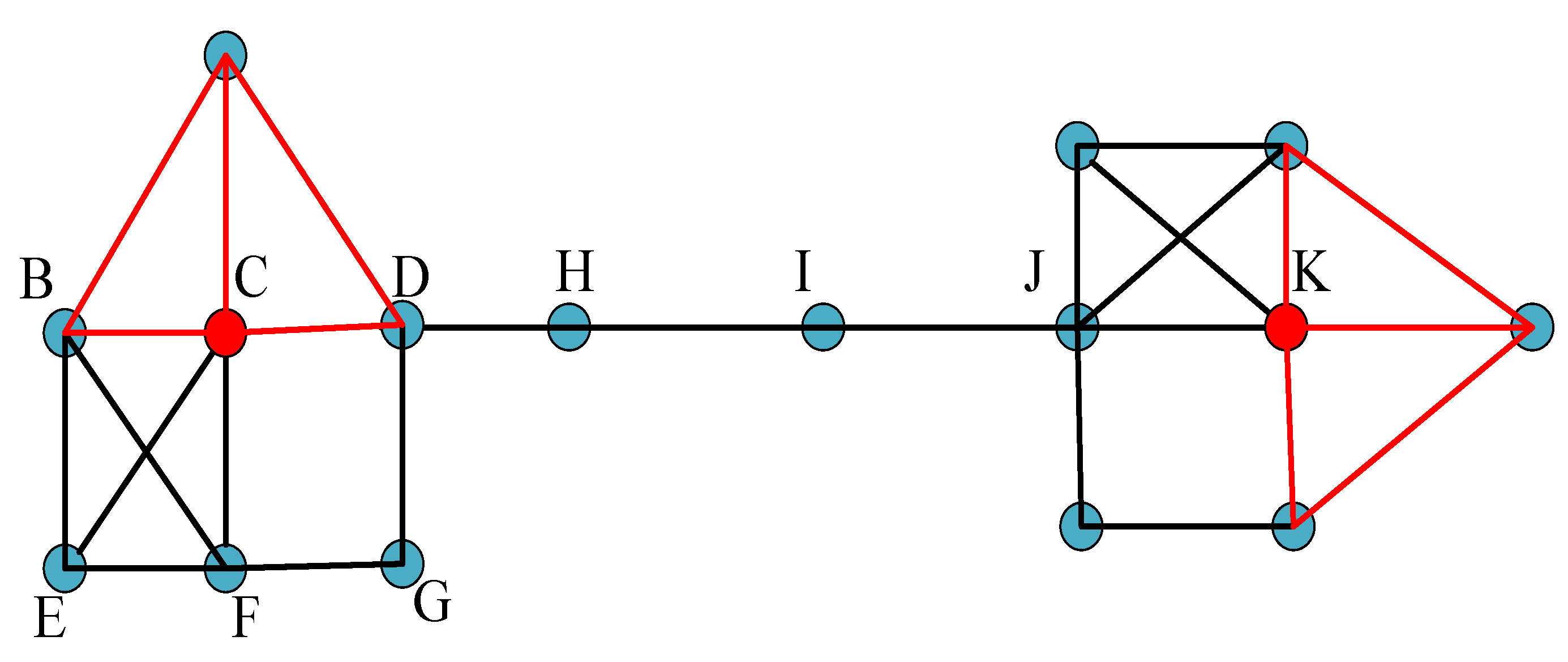
The second phase is to formulate the clusters based on the highest CC values of target nodes. Clustering helps to minimize the number of computations for anchor nodes in localization process which also minimize the radiation distance among unknown nodes and anchor nodes. Clustering schemes splitting the networks in separates groups of nodes individually cantering around maximum CC value. In SNA based solution, the selected number of anchors are not less than four to perform trilateration. By increasing the number of anchor nodes, the more clusters are formulated that even increased the localization accuracy.

Let us consider four anchor nodes $V_1,V_2,V_3,V_4$, which only form one cluster in a network. But as per modulation process if there are five anchors $V_1,V_2,V_3,V_4,V_5$, it can forms five clusters in a best case scenario. With five possible combinations, we have $(V_1,V_2,V_3,V_4)$, $(V_1,V_2,V_3,V_5)$, $(V_1,V_2,V_4,V_5)$, $(V_1,V_3,V_4,V_5)$, $(V_2,V_3,V_4,V_5)$ different clusters as described in Figure 4 taken from Reference [36].

The relationship between number of anchor nodes and number of clustered is computed by:

$${\tau }_n=C(\mathsf{\Psi },V){=}^{\mathsf{\Psi }}{C}_V=\frac{\mathsf{\Psi }!}{V!(\mathsf{\Psi }-V)!},$$

(17)

where ${\tau }_n$ denotes the number of clusters formulated by the available number of anchor nodes, $\mathsf{\Psi }$ is the set of anchors and V is the minimum number of anchors used for trilateration process. As demonstrated in Figure 5, the closest anchors to unknown node $N_1$ are the nodes in cluster $C_1$, which is marked by red dotted circle, and these nodes are $(V_1,V_2,V_3,V_4)$. All other clusters $(C_2,C_3,C_4,C_5)$ are far from the unknown node $N_1$, it is not feasible to complete trilateration process with those anchor nodes. But if a node in a cluster $C_1$ is damaged due to some software or hardware error, it can make a new cluster after sending modulation signal having node ID to the possible nearest node, leading to high localization error in trilateration process.

The algorithm of clustering phase is described in Algorithm 2.

Algorithm 2 Clustering Phase

1: get number of available clusters from (17) $C_n$ 2: for$n=1:C_n$do 3:  calculate central point of each cluster by taking average of each $X,Y,Z$ for the four anchor nodes in a given cluster = $C_p$. 4: end for 5: for$k=1⟶V_n+1:N_1$do 6:  initialize minimum distance $d_m=N_1⟶C_p$ 7:  for $n=1:C_n$ do 8:   for all clusters set minimum distance $d_m$. 9:  end for 10: end for 11: for$l\to d_{m}1:4$do 12:  measure distance between each unknown node and anchor node. 13:  get RSSI for trilateration in next step. 14:  measure the noisy signal data for overall performance. 15: end for

Definition 2.

Given a graph, $G(\mathsf{\Psi },V_{\zeta })$ with every vertex distance is 1. $v\subset V$ is a $\mathsf{\Psi },V_{\zeta }$ cluster if the following conditions are true.

1.

Indegree: $\forall v\in V,\mid G(v,V)\mid \ge V_{\zeta }\mid V$

2.

Outdegree: $\forall n\in N,\mid G(n,N)\mid \ge V_{\zeta }\mid N$.

5.3. Localization Computation

After selecting the closest cluster to the unknown target from all available clusters, trilateration process takes place to localize the unknown node. Consider anchor nodes $(V_1,V_2,V_3,V_4)$ having distance $(d_1,d_2,d_3,d_4)$ as shown in Figure 5, the spheres equations are:

$$d_a^2={(x-x_a)}^2+{(y-y_a)}^2+{(z-z_a)}^2$$

(18)

$$d_b^2={(x-x_b)}^2+{(y-y_b)}^2+{(z-z_b)}^2$$

(19)

$$d_c^2={(x-x_c)}^2+{(y-y_c)}^2+{(z-z_c)}^2$$

(20)

$$d_d^2={(x-x_d)}^2+{(y-y_d)}^2+{(z-z_d)}^2.$$

(21)

In further expansion the above equations can be written as in final matrix form [16]:

$$\left[\begin{array}{ccc}{X}_{da}& Y_{da}& Z_{da}\\ X_{db}& Y_{db}& Z_{db}\\ X_{dc}& Y_{dc}& Z_{dc}\end{array}\right]\left[\begin{array}{c}x\\ y\\ z\end{array}\right]=\left[\begin{array}{c}u\\ v\\ w\end{array}\right].$$

(22)

In this phenomenon anchor node $V_5$ is beyond the cluster of target node $N_1$. The RSSI value and cluster information is used in trilateration process to compute the node position using (22). The error in localization is given by:

$$d_{error}=\sqrt{{(xe-\widehat{x})}^2+{(ye-\widehat{y})}^2+{(ze-\widehat{z})}^2},$$

(23)

where $\widehat{x},\widehat{y},\widehat{z}$ are the estimated values of the target node. The average localization error is then measured by $E_{avg}=d_{error}/N$.

The algorithm of Trilateration and error calculation is described in Algorithm 3.

Algorithm 3 Trilateration and error calculation

1: Calculate $N_{xe},N_{ye},N_{ze}$∀$N_n$ using Equation (22). 2: initialize localization error ⟶$Err.sum=0$ 3: for$k=1⟶V_n+1:N_1$do 4:  Calculate error ∀$N_n$ using Equation (23). 5:  $err.sum=err.sum+E\left(k\right)$ 6: end for 7: $Avg(err.sum)=err.sum/totalnoofnodes$

Average localization error provides a general indication of the accuracy of the overall system. Our target is to minimize the localization error and enhance the performance of proposed solution. CC is very helpful in measuring the node’s distance, with minimal computation load on the target side. Most of the computational load is with the anchor nodes, thus reducing the computational and energy cost for other nodes.

6. Simulation Results

For the setup of simulation, sensors are randomly deployed in $1000\mathrm{m}\times 1000\mathrm{m}\times 500\mathrm{m}$ working space as shown in Figure 5. It simulates an indoor WSN that has V anchor nodes and N target nodes.

6.1. Accuracy Analysis

Random deployment makes the localization algorithm more robust for different network topologies. In our simulation, the path loss exponent is set to $\gamma =3$ and power loss $L_0=40$ dB. The performance metric of our proposed algorithm is based on CC values. Root mean square error (CCRMSE) is defined as:

$$CCRMSE=\sqrt{\frac{1}{CC}\sum _{(i,j)=1}{\Vert x_{i,j}-{\tilde{x}}_{i,j}\Vert }^2}.$$

(24)

We choose 100 anchor nodes and 160 unknown nodes. The CC between the nodes are computed by Equation (11). The nearest cluster is chosen based on the highest CC value. The highest CC valued anchor nodes and associated cluster can further select three nodes for trilateration. The anchor nodes $V_1,\dots ,V_4$ form a cluster for node $N_1$ due to having the highest CC and nearest cluster as shown in Figure 4. The target node $N_1$ is only at a distance of 1m from $V_1$. Let us consider another scenario, if the node $V_1$ is damaged then system needed to calibrate at a certain period of time [37]. In this case the formulation of the new cluster and computation of the highest CC value is required. The formulation of cluster and CC computation is shown in Figure 6. It shows that there might be 70 possible clusters in the case of 8 anchor nodes, which is computed by Equation (17).

6.2. Localization Error

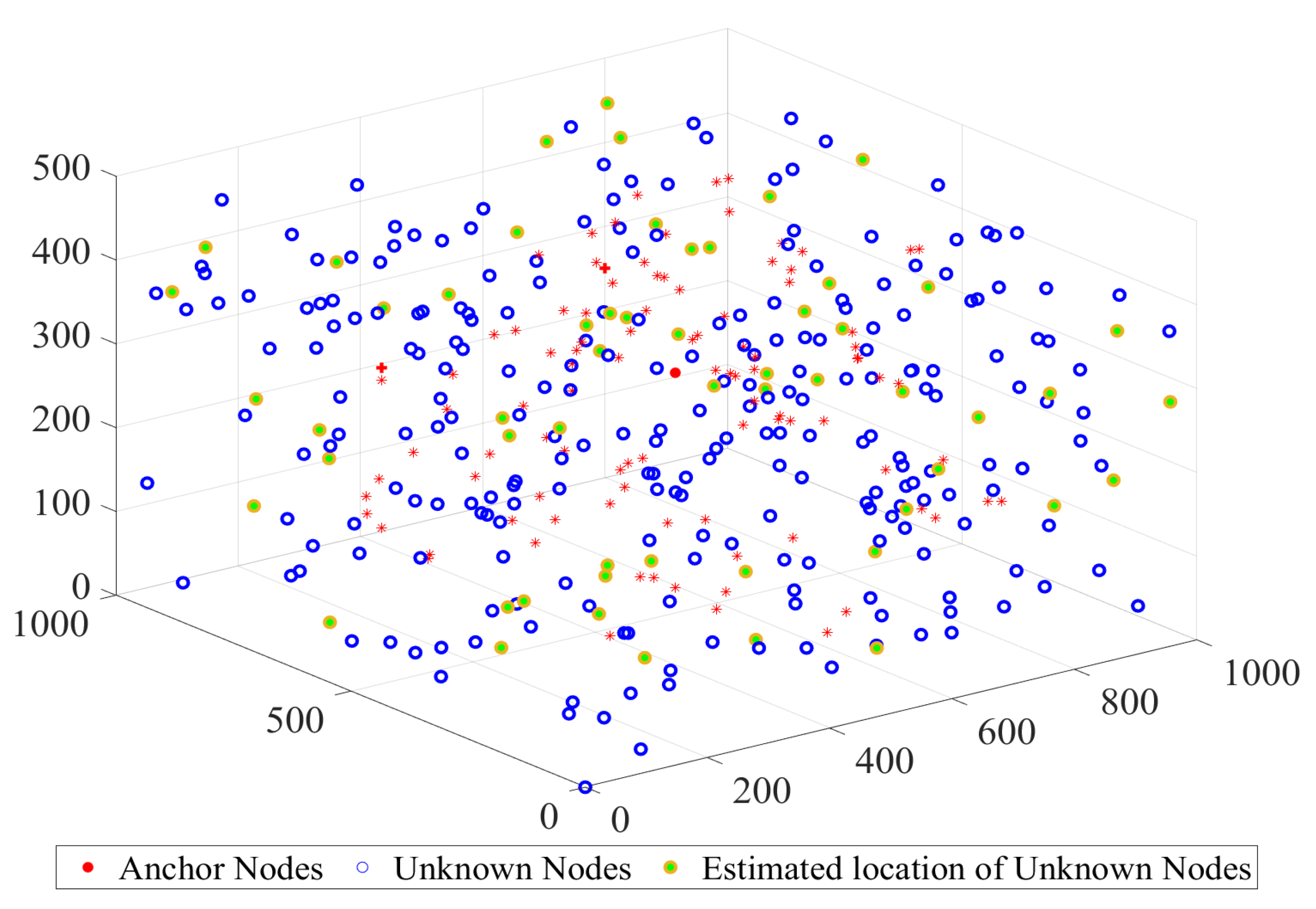
The initial deployment of anchor nodes, target nodes and estimated position of target node is shown in Figure 7. The simulation is performed using the RSSI data set obtained from github geolife trajectories [38]. The accuracy of the CC based metric is directly proportional to the highest clustered values from the RSSI data set. 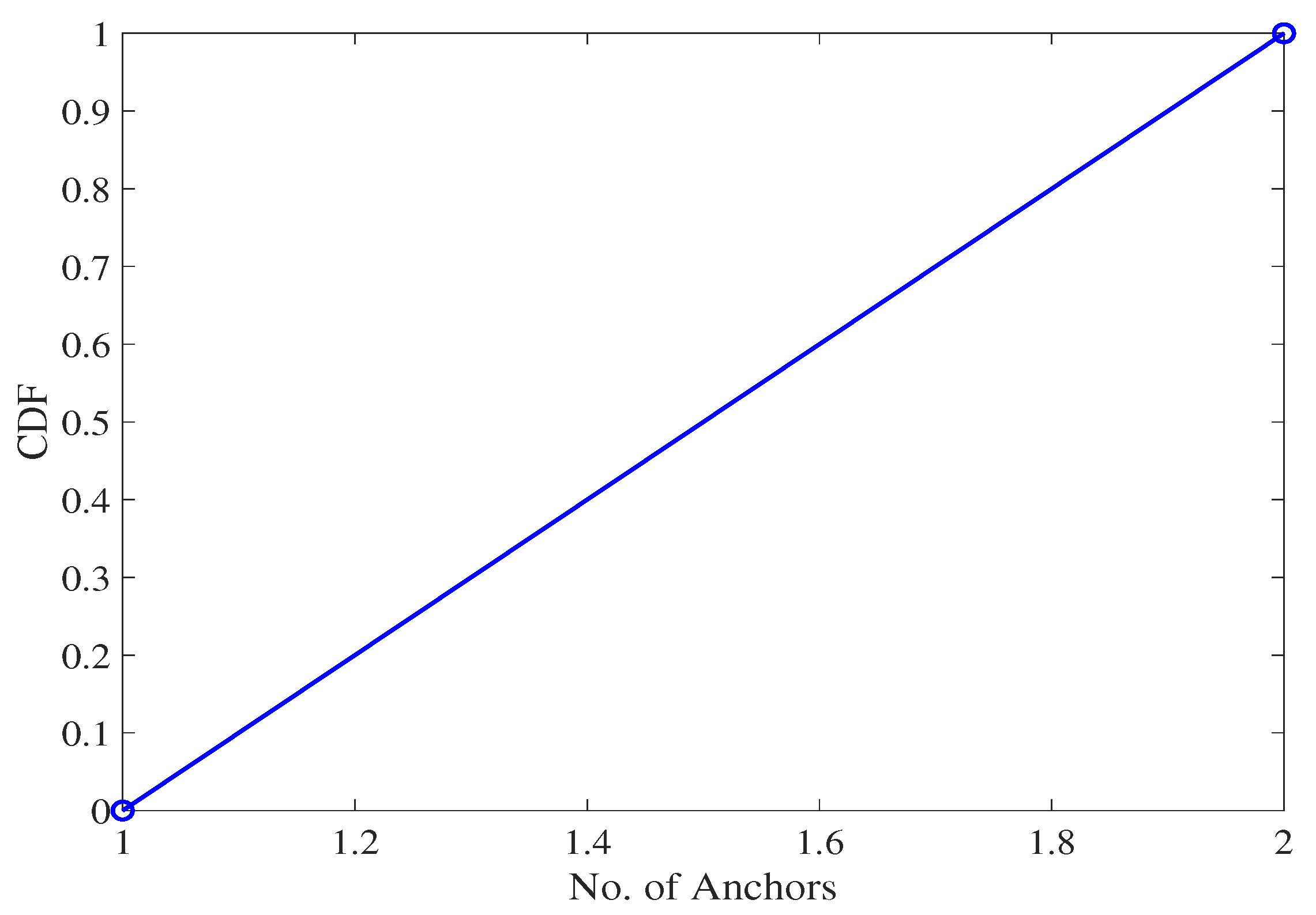The simulation shows that the localization error of the SNA based algorithm on each axis is about $0.32$ m and the average localization error of $1.35$ m by trilateration as shown in Figure 8 with a CDF plot in Figure 9.

The CDF is a statistical tool that gives indication of probability for the average localization error $P_r$ to take value with in the range of $p=[0,1]$ given by the relation:

$$CDF\left(P_r\right)=P(P_r\le a)$$

(25)

$$P(0<P_r\le 1)=CDF\left(1\right)-CDF\left(0\right).$$

(26)

For further analysis of the anchor nodes’ density, the number of anchor nodes is increased gradually to check the system performance. It is understood that the localization error decreases due to a lot of clusters in the presence of higher number of anchor nodes.

The communication cost is one of the crucial and significant factors that affects the performance of the WSN localization technique, especially when using sensors with high power consumption. It differs from the computation cost because computation cost refers to the cost of calculation processes between nodes and anchors, the communication cost deals with the energy of transmitting, receiving, listening, sleeping and switching. For the communication cost modeling, the standard that is used here to cover the test area will be 802.11 g, which can cover a range of 1000 m, with transmission power of 2.3 mW and receiving power of 1.9 mW. For transmitting and receiving energy they are $42.59$ nJ/bit, and $35.19$ nJ/bit, respectively. The system contains N sensor nodes that are identical in communication range r and having a unique ID. The test area is homogeneous. Our model for communication cost is denoted as $E_c$:

$$E_c=E_{tx}+E_{rx}+E_{lis}+E_{sw}+E_{slp},$$

(27)

where

$E_{tx}$ is the amount of energy required to transmit the data.

$E_{rx}$ is the energy consumption while receiving the data packet.

$E_{lis}$ is the energy consumption by the sensor while it is active but not receiving and transmitting any data packet.

$E_{sw}$ defines the switching energy state for the anchor nodes.

$E_{slp}$ is the energy for switching state from sleeping mode to either transmission or receiving mode.

$$E_{Tx}=P_{Tx}\times L_{Tx}\times T_{1bit},$$

(28)

where $P_{Tx}$ is the power required to transmit data, $L_{Tx}$ is the length of transmitted packet and $T_{1bit}$ represents the time to transmit 1 bit at certain period of time.

$$E_{Rx}=P_{Rx}\times L_{Rx}\times T_{1bit},$$

(29)

where $P_{Rx}$ is the power consumption during receiving state and $L_{Rx}$ is the length of received data packet.

$$E_{Lis}=P_{Lis}\times T_{Lis},$$

(30)

where $P_{Lis}$ is the power consumed when the sensor in the mode of listening and $T_{Lis}$ is the periodical time between the states of being listening for the sensor.

$$E_{Sw}=Avg\left(P_{Sw}\right)\times T_{Sw},$$

(31)

where $P_{Sw}$ is the power required when the sensor switches from one state to another one, while $T_{Sw}$ is the switching time between these states.

$$E_{Slp}=\left(P_{Slp}\right)\times T_{Slp},$$

(32)

where $P_{Slp}$ is the power through sleeping mode for the sensor and $T_{Slp}$ is the sleeping time.

6.3. Effect of Rayleigh Fading and Noise

From the central limit theorem, RSSI can also be represented through Rayleigh PDF and Gaussian random complex variable given by [39]:

$$f_X\left(x\right)=\frac{x}{{\sigma }^2}\times e^{-\frac{x^2}{2{\sigma }^2}},$$

(33)

where ${\sigma }^2$ is a component manipulating the Rayleigh factor. ${\sigma }^2$ is set to be $0.5$ with $E\left(x^2\right)=1$ which describe the Rayleigh process with zero gain. The Rayleigh fading effect is also in our consideration to check the performance of our proposed system. RSS shows different and unique characteristics on variations in signal amplitude over time and frequency caused by fading. At first, we assume all the nodes in a network are stationary, without any noise and fading having $f_X\left(x\right)=1$. Conversely, when fading is present, the power samples is multiplied with $x^2$, where x is a random variable for fading amplitude presented in (33).

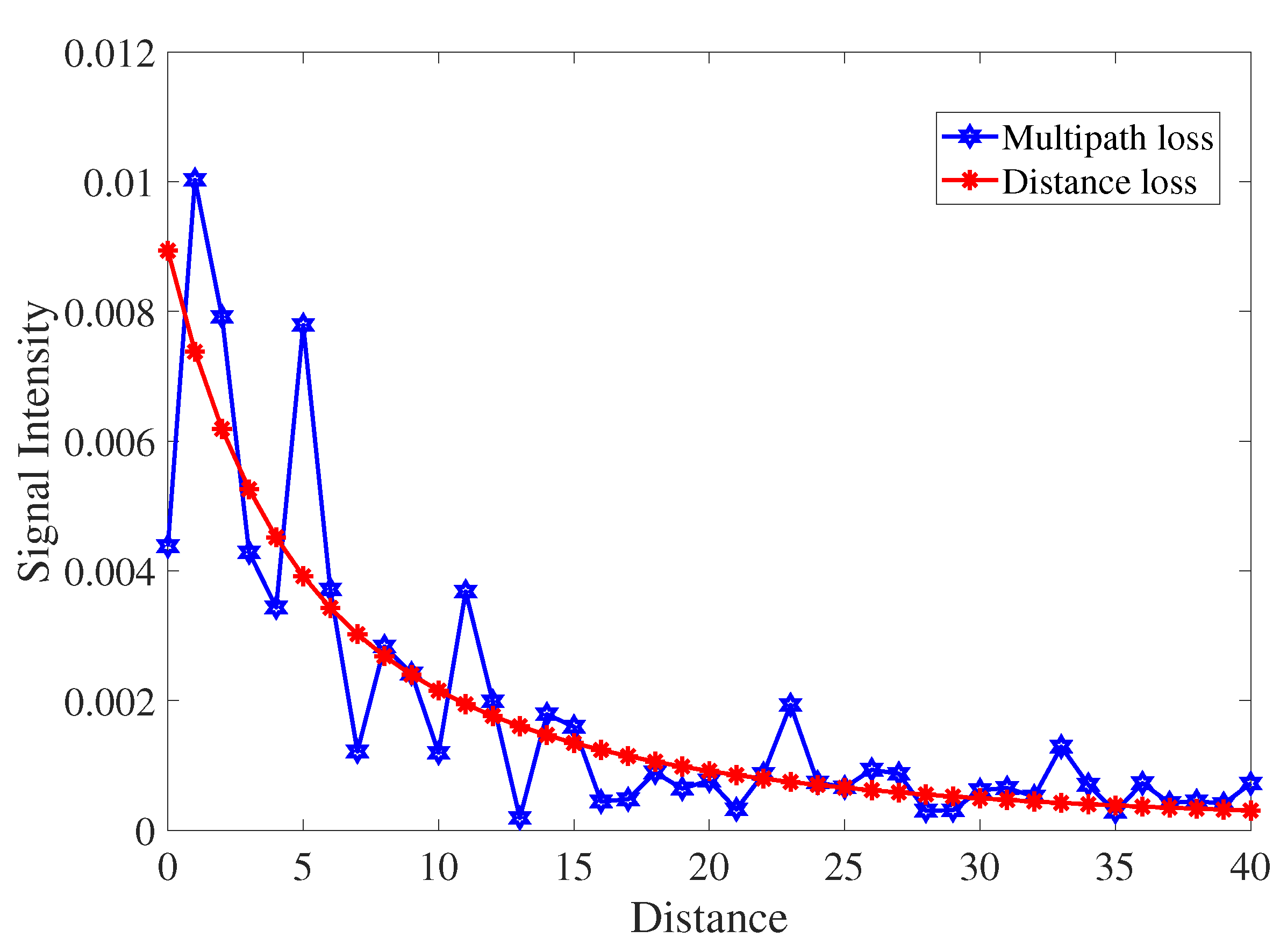
Two main properties of radio irregularity, namely continuous variations and non isotropic, the path loss is adjusted based on $\mu$ the mean, and $\sigma$, the standard deviation of the form $d=d_0+N(\sigma ,\mu )$. When studying CC, we consider 150 anchor nodes and 90 other unknown nodes to check the performance of the proposed localization scheme after adding Rayleigh fading as shown in Figure 10. The results are from 1000 iterations and we observed a slight change in overall performance of the system. This change does not affect the performance of the system due to closeness centrality test after a certain period of time. The signals are attenuated between sender and receiver in any communication channel. To obtain the RSSI characteristics, we measured RSSI at different distances up to 1000 m. The noise also affects the signal intensity as shown in Figure 11. Furthermore, transmission loss is measured by adding power factor to the CC values. For non least square fitting to a Gaussian function, we squared the CCRMSE from (24).

6.4. Comparison with Existing Methods and Computational Complexity

It is interesting to compare our results with the other 3D based localization techniques discussed in Section 2. First we discussed the performance of traditional APIT algorithm. In APIT, if a node is away from the triangle and unknown node, it is presented outside the triangle so the test fails and the node do not localized. Obviously, this selection is very important as neighbor node play an important role in selection of the triangles. This problem is solved in the proposed SNA algorithm where the node can select the nearest anchor node if a node is failed or down next to it. The ties between the clustered area is also increased and have a chance to localize multiple nodes within a cluster which also overcome the computation cost.

MDS-MAP is a classical multidimensional mathematical scaling that has origins in psychophysics and psychometrics. The distance is expressed like geometrical pictures shown as an information visualization or exploratory data. Therefore the complexity of MDS is always very high due to extra mathematical computation giving a time computation of $O\left(n^3\right)$. In simple scenarios the localization accuracy is above 2 m where distance between every pair of nodes is crucial. The SNA based idea also overcomes the pair computation and ties up with the new relation even if a node fails. That is why there is a $72\%$ improvement in our proposed solution.

For evolution purposes, two different topologies—C-shaped and uniformly distributed square regions—are considered to check the network coverage area while increasing the connectivity level, number of anchors and sensor nodes and distance between different anchor pairs. The connectivity level was increased between 11 and 31 by changing the radio range. The simulation was run for 1000 times and almost $98\%$ and record the localization error. The error in case of MDS-MAP and DV-Hop is above 2 m in some cases. While the use of clustering in our proposed solution is below $0.5$ m. The worst-case complexity for SNA based algorithm is derived from interior algorithms [40]. The SNA provides a unique solution when having $O\left(n\right)$ pair of nodes with a known distance. However the use of CC as a SNA reduce the overall complexity of proposed solution. Even in the case of node failure the SNA calibrates itself and forms a new cluster to run the process of localization efficiently.

The average localization error was obtained after 1000 iterations. We noticed that clustering of the social network gives high performance rather than some existing methods like DV-Hop, and MDS-Map and advanced DV-Hop schemes as shown in Figure 12.

7. Conclusions

Node localization plays a vital role in providing meaningful data in most applications of WSNs. Many researchers proposed 2D based localization algorithms; however, most of them are based on the assumptions of accurate synchronization between sensor nodes, which can be difficult or sometimes impossible to achieve in an uncontrolled environment. This paper proposed a novel 3D localization algorithm based on the well-known Social Network Analysis algorithm, which is free from node synchronization and thus only requires determination of the Closeness Centrality to form a clustering for trilateration. The simulation results shows that the proposed SNA-based localization algorithm can achieve an average error distance as low as $0.32$ m, which can be further reduced while increasing the node density. The idea of SNA based on CC provides high accuracy where less computation is required in order to achieve high accuracy with low energy consumption.

However, there is still some room for further studies, such as the impact of anchor node localization error. It is also worth studying how to adopt mobile anchor nodes to further improve the localization accuracy.