Onboard Visual Horizon Detection for Unmanned Aerial Systems with Programmable Logic

Abstract

We introduce and analyze a fast horizon detection algorithm with native radial distortion handling and its implementation on a low power field programmable gate array (FPGA) development board in this paper. The algorithm is suited for visual applications in an airborne environment, that is on board a small unmanned aircraft. The algorithm was designed to have low complexity because of the power consumption requirements. To keep the computational cost low, an initial guess for the horizon is used, which is provided by the attitude heading reference system of the aircraft. The camera model takes radial distortions into account, which is necessary for a wide-angle lens used in most applications. This paper presents formulae for distorted horizon lines and a gradient sampling-based resolution-independent single shot algorithm for finding a horizon with radial distortion without undistortion of the complete image. The implemented algorithm is part of our visual sense-and-avoid system, where it is used for the sky-ground separation, and the performance of the algorithm is tested on real flight data. The FPGA implementation of the horizon detection method makes it possible to add this efficient module to any FPGA-based vision system.

1. Introduction

Unmanned aerial vehicle systems (UAS) with an airborne camera are used in more and more applications from the aerial recreational photo shooting, to more complicated semi-autonomous surveillance missions, for example in precision agriculture [1]. Safe usage of these autonomous UAS requires Sense and Avoid (SAA) capability to reduce the risk of collision with obstacles and other aircraft. Surveillance mission setups include onboard cameras and a payload computer, which can also be used to perform SAA. Thus, computationally cheap camera-based solutions may need no extra hardware component. Most of the vision-based SAA methods use different approaches for intruders in sky and land backgrounds [2,3,4]. Thus, they can utilize horizon detection to produce fast sky segmentation. Attitude heading reference system (AHRS) is a compulsory module of UAS which provides Kalman-filtered attitude information from raw IMU (Inertial Measurement Unit) and GPS measurements [5,6,7]. This attitude information can enhance the sky-ground separation methods, because it can give an estimate of the horizon line in the camera image [8]; furthermore, if the horizon is a visible feature (planar scenes), it can also be also used to improve the quality of attitude information [9] or support visual serving for fixed-wing UAV landing [10]. Sea, large lakes, plains, and even a hilly environment at high altitudes give visible horizon in the camera view, which is worth detection onboard.

There are several solutions for horizon detection in the literature. In general, more sophisticated algorithms are used, which use a statistical model for the sky and non-sky region separation. Ettinger et al. use the covariance of pixels as a model for the sky and ground [11], while Todorovic uses a hidden Markov tree for the segmentation [12]. McGee et al. [13] and Boroujeni et al. [14] use a similar strategy, where the pixels are classified with a support vector machine, or with clustering. A different kind of strategy is followed by Cornall and Egan [15] and Dusha et al. [16] Cornall and Egan [15] use various textures, and they only calculate the roll angle. Dusha et al. [16] combine optical flow features with Hough transform and temporal line tracking, to estimate the horizon line. The problem with the single line model is that it cannot efficiently estimate the horizon in the case of tall buildings, or trees and high hills, where the horizon can be better modeled with more line segments. Shen et al. [17] introduced an algorithm for horizon detection on complex terrain. Pixel clustering methods, in general, have the potential to give sky-ground separation in any case, but they are computationally expensive. Notably, [18] presents a real-time solution that considers sky and ground pixels as fuzzy subsets in YUV color space and continuously trains a classifier above this representation and compares its output to precomputed binary codes of possible attitudes. This approach can be very effective if ground textures do not change fast during flight and the camera always sees the horizon. To overcome this problem, the authors used two 180-degree field of view (FOV) cameras. Their image representation was only 80 × 40 pixel, but the straight line horizon is a large feature and can be detected in such low resolution.

SAA and most of the main mission tasks need high-resolution images for the detection of small features and aim for high angular resolution at large FOV. With a simple down-sampling, one can provide input for existing horizon detection methods that work on low-resolution images, but we can reach higher accuracy in the original image, which has a fine angular resolution. We still need to do other manipulations in the high resolution for SAA and main mission tasks; thus, using this has no overhead. In our previous work [8], a simple intensity gradient sampling method was proposed, which fine-tunes an initial horizon line coming from the AHRS attitude. The computational need is only defined by the number of sample points and is independent from the image resolution. The single-shot approach is more stable, because detection errors cannot propagate to consecutive frames. The existence of a horizon can also be defined based on the AHRS estimate. This horizon detector was utilized in our successful SAA flight demonstration [2].

Large FOV optics have radial distortion, which does not degrade the detection of small features (intruder). However, it makes horizon detection challenging without complete undistortion of the image. In this paper, we introduce the advanced version of [8] with native radial distortion handling, in which only a few numbers of feature/sampling points need to be transformed, instead of the complete image. The mathematical representation of the distorted horizon line is given with the experimental approach to finding it. The method is evaluated on real flight test data. This paper presents the field programmable gate array (FPGA) implementation of the novel horizon detection module, with a theoretic complete vision system for SAA.

2. Horizon Detection Utilizing AHRS Data

The attitude heading reference system provides the Euler angles of the aircraft, which define ordered rotations around the reference North-East-Down coordinate system. First, it takes a rotation around Down (yaw), then a rotation around the rotated East (pitch), and finally, a rotation around the twice rotated North (roll), to have the actual attitude of the aircraft. We can also calibrate once the relative transformation of the camera coordinate system to the aircraft body coordinate system. With this information, one can define a horizon line in the image, which has calibration and AHRS errors. In this paper, we use this AHRS-based horizon as an initial estimation of the horizon line in the image.

2.1. Horizon Calculation from AHRS Data

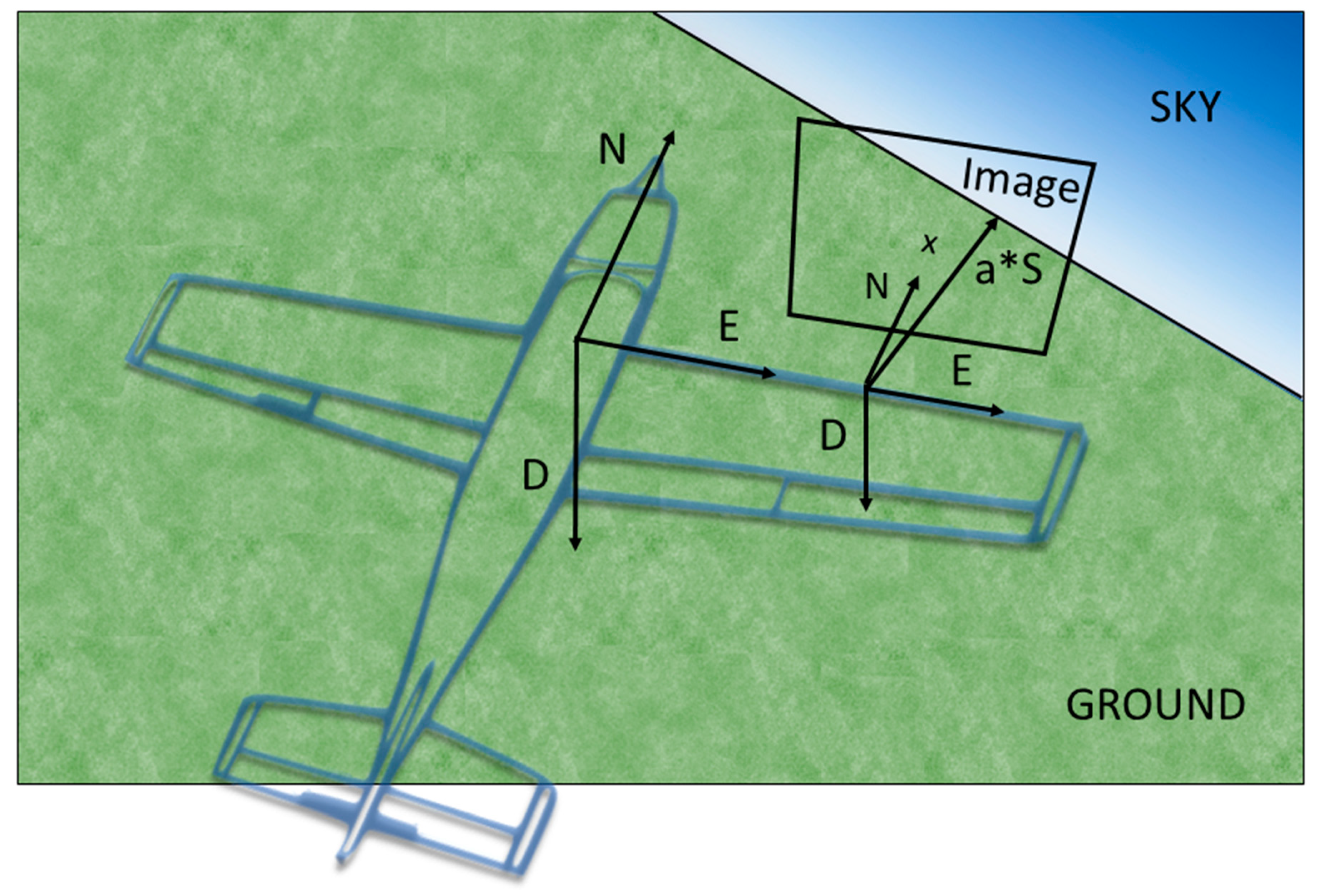
Figure 1 presents the main coordinate systems and the method for horizon calculation form Euler angles. We define one point of the horizon in the image plane and the normal vector of it. To reach this, we transform the North (surface parallel) unit vector of world coordinate system to the camera coordinate system and get its intersection with the image plane, which will be one point of the horizon (it can be out of the borders), and we can also transform a unit vector pointing upwards in the world reference to have a normal vector as the projection of transformed upward vector to the image plane. The horizon line is given by a point $P_0$ and a normal vector $\overrightarrow{n}$ [8].

2.2. Horizon Based on AHRS Data Without Radial Distortion

The horizon is a straight line, if we assume a relatively unobstructed ground surface (flats, small hills, lakes, sea), with a negative intensity drop from the sky to ground, in most cases. Infrared cut-off filters can enhance this intensity drop, because it filters out infrared light reflected by plants. In general, because of the different textures on the images, the horizon cannot be found solely based on this intensity drop.

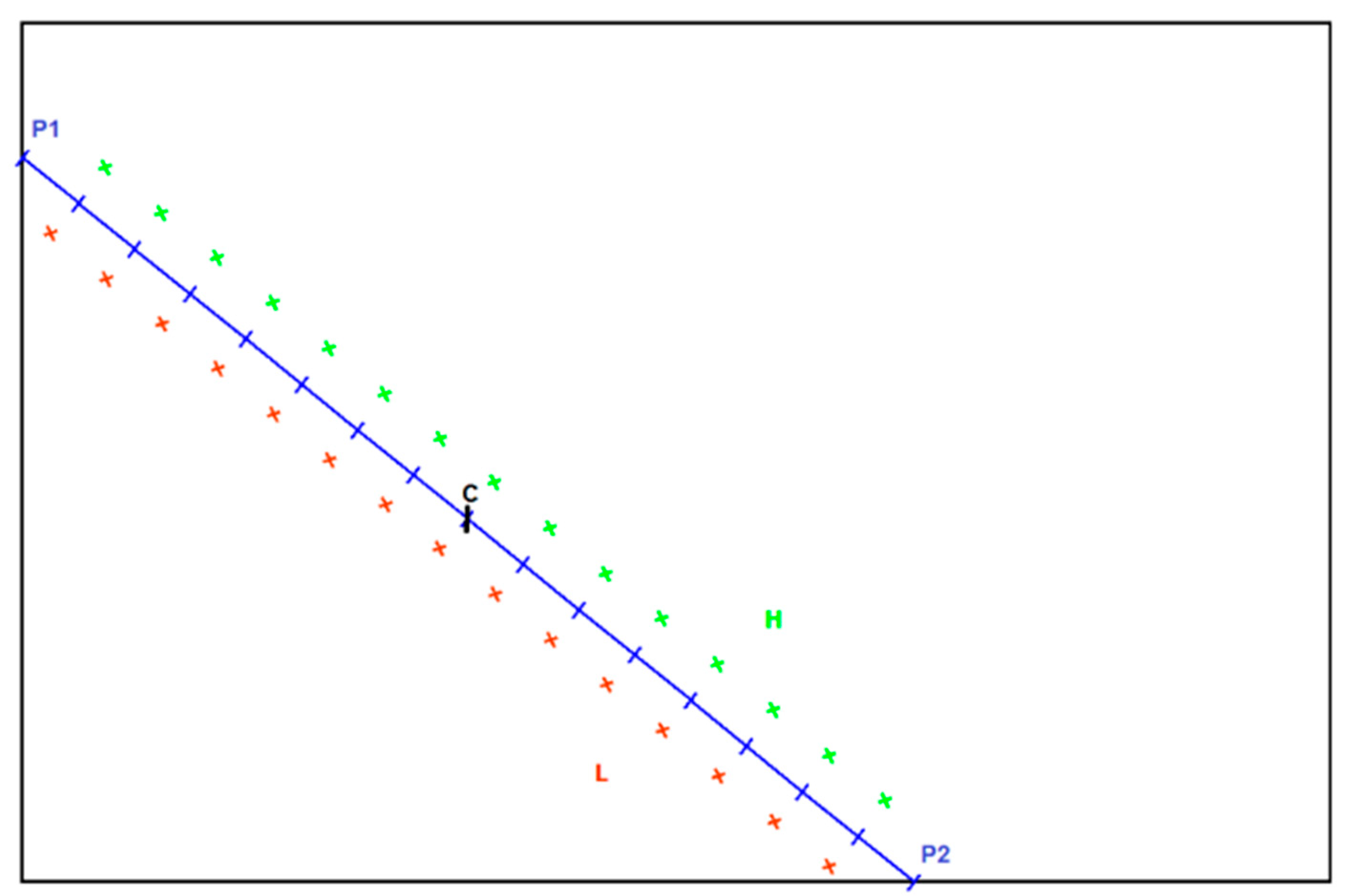
On the other hand, with AHRS data, an initial guess for the horizon line’s whereabouts is available. This estimate is within a reasonable distance from the horizon in most cases. Thus, it can guide a search for the real horizon line on the image plane. Rotations around the center point of the line and shifts in the direction of its normal vector are applied to get new horizon candidates. Every time, the intensity drop is checked at given points, denoted by H (sky region) and L (ground region), as it is shown in Figure 2. The algorithm to find the horizon, in this case, is described in more detail in [8]. In this paper, we introduce the advanced version of this gradient sampling approach, which considers the radial distortion of large FOV cameras.

2.3. Exact Formula of Distorted Horizon Lines

A standard commercial camera usually realizes the perspective projection. Consequently, the projection of the horizon is a straight line in the image space. However, perspectivity is only an approximation of the projection of real-world cameras. If a camera is relatively inexpensive or it has optics with a wide field of view (FOV), then more complex camera models should be introduced. A standard solution is to apply the radial distortion model to cope with the non-perspective behavior of cameras.

We have selected the 2-parameter radial distortion model [19] in this study. Using the model, the relationship between the theoretical perspective coordinates $\begin{array}{cc}[u & v\end{array}{]}^T$ and the real ones $\begin{array}{cc}[u^{\prime } & v^{\prime }\end{array}{]}^T$ is given as follows:

$$\left[\begin{array}{c}u\prime \\ v\prime \end{array}\right]=\left(1+k_1{r}^2+k_2{r}^4\right)\left[\begin{array}{c}u\\ v\end{array}\right],$$

where $k_1$ and $k_2$ are the parameters of the radial distortion, and $r=\sqrt{u^2+v^2}$ gives the distance between the point $\begin{array}{cc}[u & v\end{array}{]}^T$, and the principal point. The principal point is the location at which the optical axis intersects the image plane. Therefore, this relationship is valid only if the origin of the used coordinate system is at the principal point. Another important pre-processing step is to normalize the scale of the axes by the division with the product of the horizontal and vertical focal length and pixel size of the camera.

The critical task for horizon detection is to compute the radially distorted variant of a straight line. Let the line be parameterized as:

$$\left[\begin{array}{c}u\\ v\end{array}\right]=\left[\begin{array}{c}{u}_0\\ v_0\end{array}\right]+t\left[\begin{array}{c}u\\ v\end{array}\right],$$

where $t$ is the line parameter, $d=\left[d_u d_v\right]$ the vector of the line’s direction. The distorted line is written by:

$$\left[\begin{array}{c}u\prime \\ v\prime \end{array}\right]=\left(1+k_1{r}^2+k_2{r}^4\right)\left[\begin{array}{c}{u}_0+t{d}_u\\ v_0+t{d}_v\end{array}\right],$$

where: $r^2=t^2\left(d_u^2+d_v^2\right)+2t\left(u_0{d}_u+v_0{d}_v\right)+u_0^2+v_0^2$, and $r^4={\left(r^2\right)}^2$. The square of the radius can be written in a more simplified form as:

$$r^2=A{t}^2+Bt+C,$$

where: $A=d_u^2+d_v^2,B=2\left(u_0{d}_u+v_0{d}_v\right)$, and $C=u_0^2+v_0^2$. Then $r^4$ is expressed as:

$$r^4=A^2{t}^4+2AB{t}^3+\left(B^2+2AC\right)t^2+2BCt+C^2,$$

Therefore, the formula $\left(1+k_1{r}^2+k_2{r}^4\right)$ is also a polynomial that is written in the following form:

$$\alpha t^4+\beta t^3+\gamma t^2+\delta t+ϵ,$$

where $\alpha =k_2{A}^2$, $\beta =k_{2}AB$, $\gamma =k_2\left(2AC+B^2\right)+k_{1}A$, $\delta =2k_{2}BC+k_{1}B$, and $ϵ=k_2{C}^2+k_{1}C+1$. The parametric formula of the line can be written in a compact form as:

$$\left[\begin{array}{c}u\prime \\ v\prime \end{array}\right]=\left[\begin{array}{c}{{\displaystyle \sum }}_{i=0}^5{a}_i{t}^i\\ {{\displaystyle \sum }}_{i=0}^5{b}_i{t}^i\end{array}\right]$$

(1)

where: $a_5=\alpha d_u$, $a_4=\alpha u_0+\beta d_u$, $a_3=\beta u_0+\gamma \beta d_u$, $a_2=\gamma u_0+\delta d_u$, $a_1=\delta u_0+ϵd_u$, and $a_0=ϵu_0$. Similarly, $b_5=\alpha d_v$, $b_4=\alpha v_0+\beta d_v$, $b_3=\beta v_0+\gamma \beta d_v$, $b_2=\gamma v_0+\delta d_v$, $b_1=\delta v_0+ϵd_v$, and $b_0=ϵv_0$.

2.3.1. Limits

For the horizon detection, the radially distorted line must be sampled within the image. For this reason, the interval for parameter $t$ must be determined in which the curve lies within the area of the image. Let us denote the borders of the image with $u_l$ and $u_r$ (horizontal), $v_t$ and $v_b$ (vertical). The corresponding values for parameter $t$ are determined by solving the 5-degree polynomials ${{\displaystyle \sum }}_{i=1}^5{a}_i{t}^i-u_l=0$, ${{\displaystyle \sum }}_{i=1}^5{a}_i{t}^i-u_r=0$, ${{\displaystyle \sum }}_{i=1}^5{b}_i{t}^i-v_t=0$ and ${{\displaystyle \sum }}_{i=1}^5{b}_i{t}^i-v_b=0$. Each polynomial has five different roots. To our experiments, only one of those is the real root; the other four complex roots, two conjugate pairs, are obtained per polynomial. The complex roots are discarded, the minimal and maximal values of all possible real roots give the limits for parameter $t$.

2.3.2. Tangent Line

Another advantage of the formula defined in Equation (1). The direction ${\mathrm{d}}_{\tan }$ of the tangent line can be determined trivially by deriving the equation. It is written as follows:

$${\mathrm{d}}_{\tan }=\left[\begin{array}{c}{{\displaystyle \sum }}_{i=0}^{5}i{a}_i{t}^{i-1}\\ {{\displaystyle \sum }}_{i=0}^{5}i{b}_i{t}^{i-1}\end{array}\right]$$

(2)

2.3.3. Example

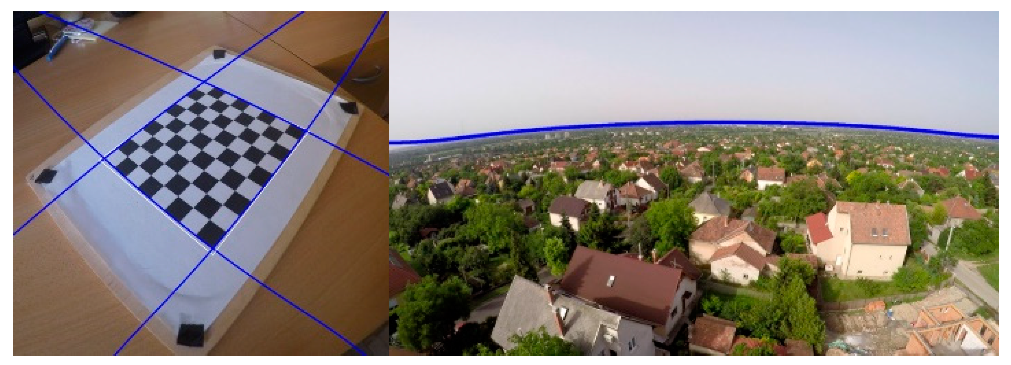
It is demonstrated in Figure 3 that the distortion model and its formulae can be a good representation of the radially distorted variant of straight lines. The test image was taken by a GoPro Hero4 camera, containing wide-angle optics. This kind of lense usually produces visible radial distortion in the images. The camera was calibrated with images of a chessboard plane, using the widely-used Zhang calibration method implemented in OpenCV3 [20]. As is expected, the curves fit the real borders of the chessboard (left image) and the horizon (right). It is well visualized that the polynomial approximation is principally valid at the center of the image. There are fitting errors close to the border, as it is seen in the right image of Figure 3. This problem comes from the fact that the corners of the calibration chessboard cannot be detected near the borders. Therefore, calibration information is not available there.

2.4. Horizon Detection, Based on AHRS Data with Radial Distortion

In the case of radial distortion, our straight-line approach [8] cannot be utilized, because the horizon’s coordinate functions are transformed into a 5th-degree polynomial in the image space. One possible way is to undistort the whole image, and then the straight-line approach is viable. However, it takes several milliseconds, even with precomputed pixel maps. The previous section describes an exact method for the distorted horizon line calculation. However, it is not necessary to calculate the exact polynomial when the algorithm investigates a candidate horizon on a distorted image. Here, we present a method that approximates the distorted horizon line with a sequence of straight lines that connects the distorted sample points of a virtual straight horizon. 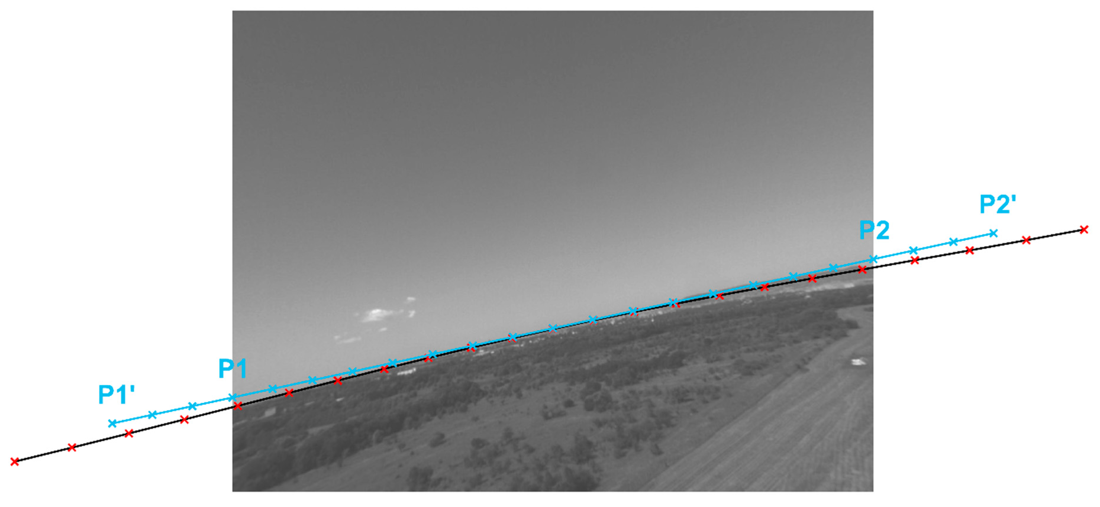Figure 4 shows the difference between an undistorted horizon line and the corresponding distorted curve.

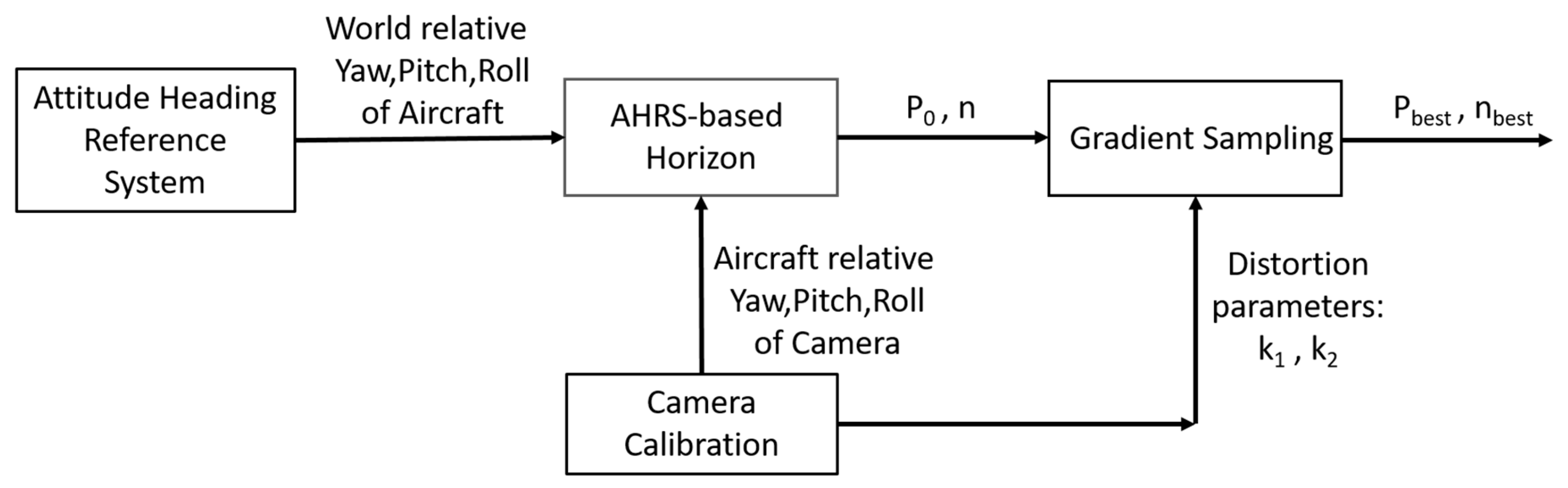
The main steps of horizon detection are the same for the distorted and the distortion-free cases, as is summarized in Figure 5. The initial AHRS-based horizon is given the same way as in the undistorted case. The pre-calculated horizon is corrected based on the distorted image, with only a few and computationally very inexpensive modifications. The gradient sampling algorithm realizes the correction mechanism based on distorted visual input. The basic idea is to create sample points at the two sides of the straight version of a horizon candidate, and distort these points to get the necessary sampling coordinates in the image (alg. gradient sampling).

Algorithm Gradient Sampling: Horizon Post-calculation with Distortion

Require: AHRS horizon line ($P_0$, $\overrightarrow{n}$), num_of_samples, step_size, deg_range, shift_range, distort_func (k1, k2) $P_1{,P}_2\leftarrow$ Two endpoints of the horizon line in the image, return if the horizon line is not on the image. $Center\leftarrow P_1+(P_2-P_1)/2$ $Base\_Points\leftarrow \mathrm{num}\_\mathrm{of}\_\mathrm{samples}$ number of equidistant sample points on the elongated AHRS horizon line fordeg = deg_range.min to deg_range.max do   Rotated_Points$\leftarrow$ Rotate Base_Points around the Center point by deg.   ${\overrightarrow{n}}_{local}$$\leftarrow$ Rotate $\overrightarrow{n}$ by deg   for $shift\_num=\mathrm{shift}\_\mathrm{range}.\min \mathbf{to}\mathrm{shift}\_\mathrm{range}.\max \mathbf{do}$   $P_{local}$$\leftarrow$$Center+shift\_num\ast step\_size\ast {\overrightarrow{n}}_{local}$   point set H $\leftarrow$Rotated_Points + $(shift\_num+1)\ast step\_size\ast {\overrightarrow{n}}_{local}$   point set L $\leftarrow$ Rotated_Points + $(shift\_num-1)\ast step\_size\ast {\overrightarrow{n}}_{local}$   point set H $\leftarrow$ distort_func (point set H)   point set L $\leftarrow$ distort_func (point set L)   Calculate the average intensity difference at points $\mathrm{H}\left(\mathrm{i}\right)\mathrm{and}\mathrm{L}\left(\mathrm{i}\right)$   Update $P_{best}$ and ${\overrightarrow{n}}_{best}$ searching for the maximal average difference return$P_{best}$, ${\overrightarrow{n}}_{best}$

The algorithm defines an exhaustive search of horizon line candidates. A predefined number of sample points are fixed on the initial pre-calculated horizon line (Base Points). These points are rotated around the center point (Rotated Points) and then shifted by the multiplicands of the rotated normal vector (${\overrightarrow{n}}_{local}$), to get H and L sample point sets for each candidate line. Finally, the sample points are distorted to have proper sampling positions in the image, which has radial distortion. 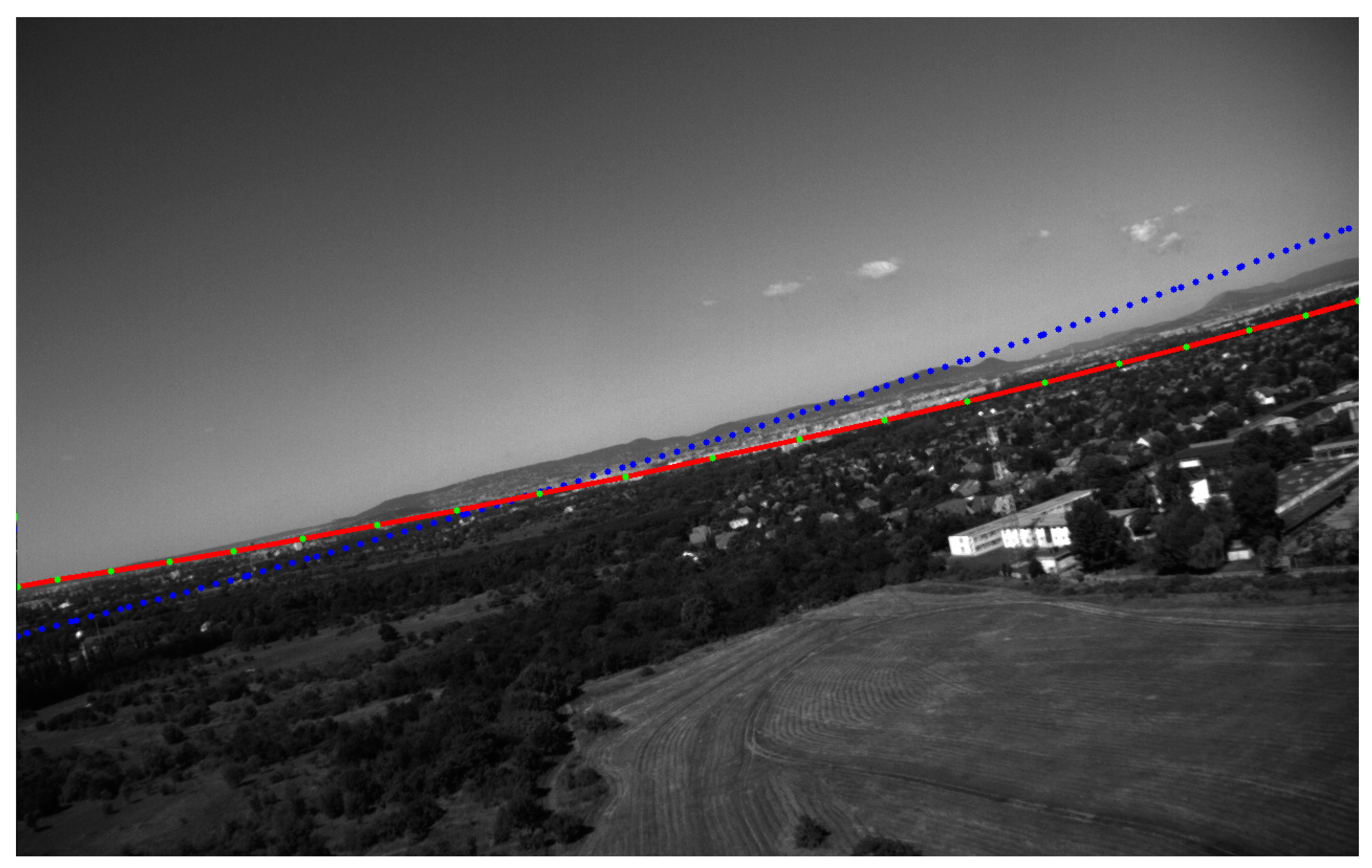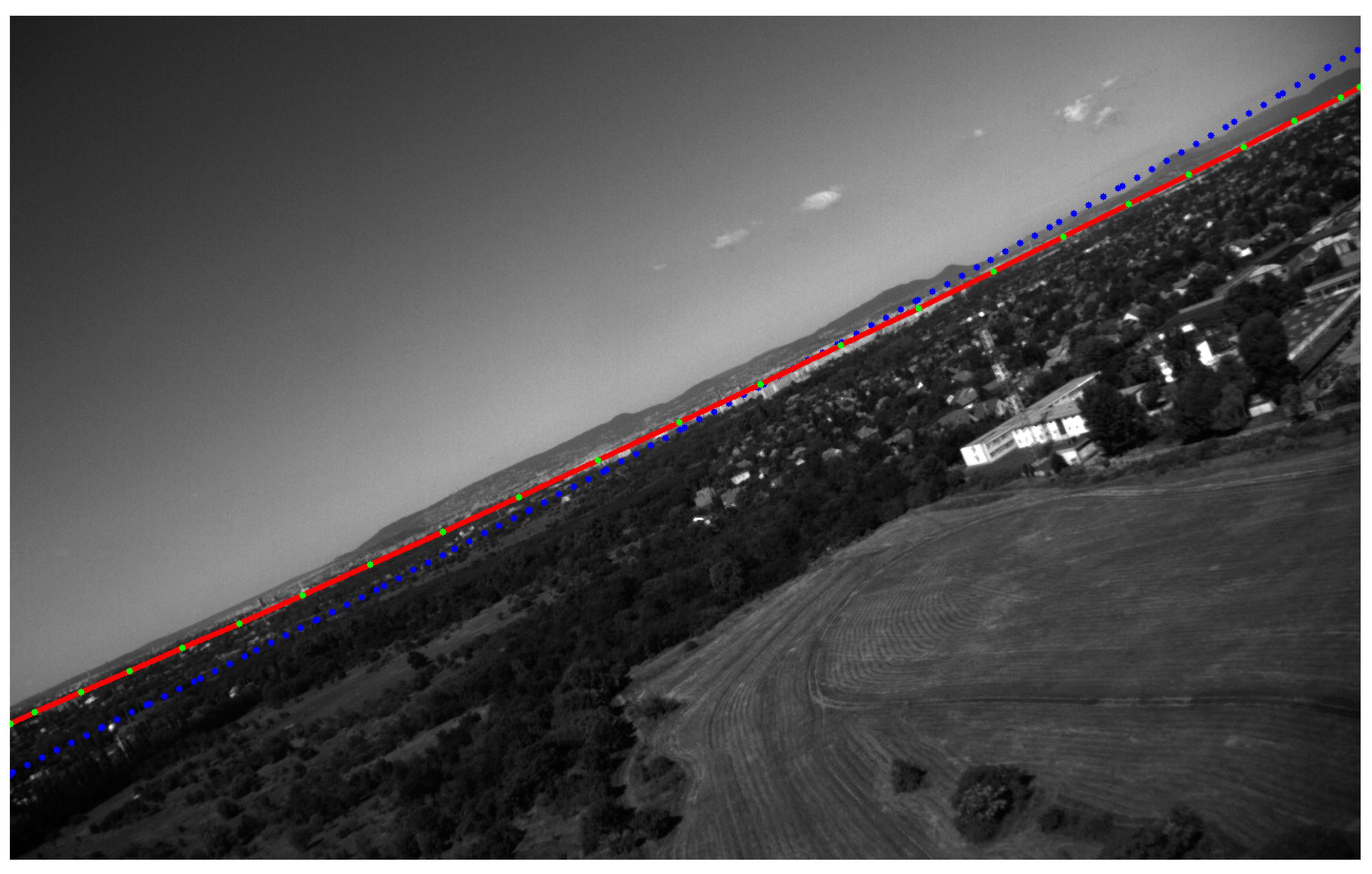The average of $img\left(H\right(i\left)\right)-img\left(L\right(i\left)\right)$ is calculated to give a gradient along with the horizon candidate. A predefined range of rotations and shifts is explored, and the line is chosen that has the largest average intensity difference on its two sides. If we consider the sample points of the straight horizon, and we connect the distorted versions of these points, it is possible that the resulted line series do not reach the borders of the image. Given that we want to get a complete horizon line, the pre-calculated straight horizon should be elongated. In our implementation, we use a rough solution by creating a 2*IMG WIDTH long line in all cases. Elements that are not in the image are discarded. Distortion and undistortion of pixel coordinates can be performed efficiently if we have a pre-computed Lookup table for the distortion of each image coordinate. Here, we need to remap only a predefined number of sample points instead of the whole image. The lines between the resulted sampling pairs (H-L) are not perfectly perpendicular to the corresponding horizon curve. However, this technique is still effective, because the L points are near below the horizon, and points in H are near above. Straight line-segments between sample points can define the horizon curve with a negligible difference from the real curve, as can be seen in Figure 6 and Figure 7.

Sky-Ground Separation in Distorted Images

In our SAA application, the horizon line is used for sky and ground separation. In the case of straight-line horizons, the masking procedure is straightforward with the help of the normal vector. However, on the distorted image, we have a series of line segments. Furthermore, the ground mask may consist of two separate parts (the horizon curve goes out and then goes back to the image). To handle this problem, we use flood-fill operation started from two inner points next to the first, and the last points of the horizon curve on the image. The masks presented in the results section were generated this way.

3. Experimental Setup

The two variants of the horizon detection algorithm (with and without radial distortion) were tested in real flights. Flights were run at the Matyasfold public model airfield, which is close to Budapest, Hungary. There are only small hills around Matyasfold, resulting in a relatively straight horizon line, which was our original assumption.

3.1. Hardware Setup of Real Flight Tests

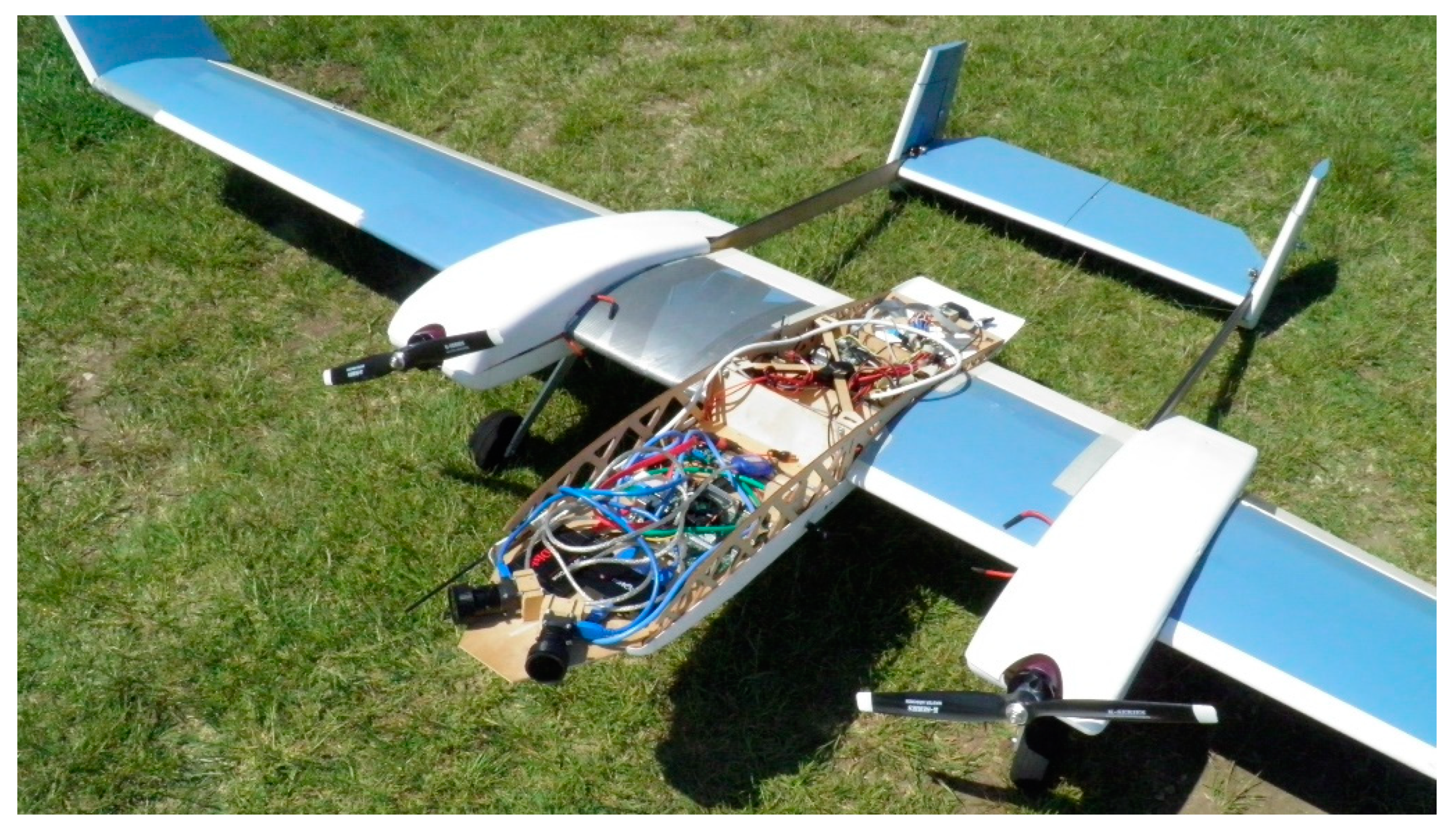
In the flight tests, a fixed-wing, two motor aircraft called Sindy was used. It is 1.85m in length, has a 3.5m wingspan, and has an approximately 12kg take-off weight (Figure 8). It is equipped with an IMU-GPS module, an onboard microcontroller with AHRS and autopilot functions (for details see [21]), and the visual sensor-processor system.

We have two embedded GPU (Nvidia TK1, TX1) and two FPGA-based (Spartan 6 LX150T [22], Zynq UltraScale+ XCZU9EG) on-board vision system hardware. The development of new algorithms is much easier on a GPU platform. However, one can have the best power efficiency and parallelization with a custom FPGA implementation. All the flight test data in this paper acquired by the Nvidia Jetson TK1 system [8] and tested offline with the new FPGA system. The two Basler Dart 1280-54um cameras have monochrome 1280 × 960 sensor and 60-degree FOV optics, where the two FOVs have a 5-degree overlap.

There are different AHRS solutions which differ in sensor types and sensor fusion technique. Different levels of AHRS quality (with and without GPS sensor) and corresponding AHRS-based horizons were analyzed in [8]. In this paper, the best available on-board estimations of Euler angles are used to create AHRS-based horizon candidates. Our Kalman-filter based estimator is described in [6], which gives Euler angles to the autopilot. However, these results can still be improved, and small calibration errors of the camera relative attitude and deformations of the airframe during maneuvers can cause additional differences between the AHRS horizon and the visible feature in the image, which makes horizon detection necessary.

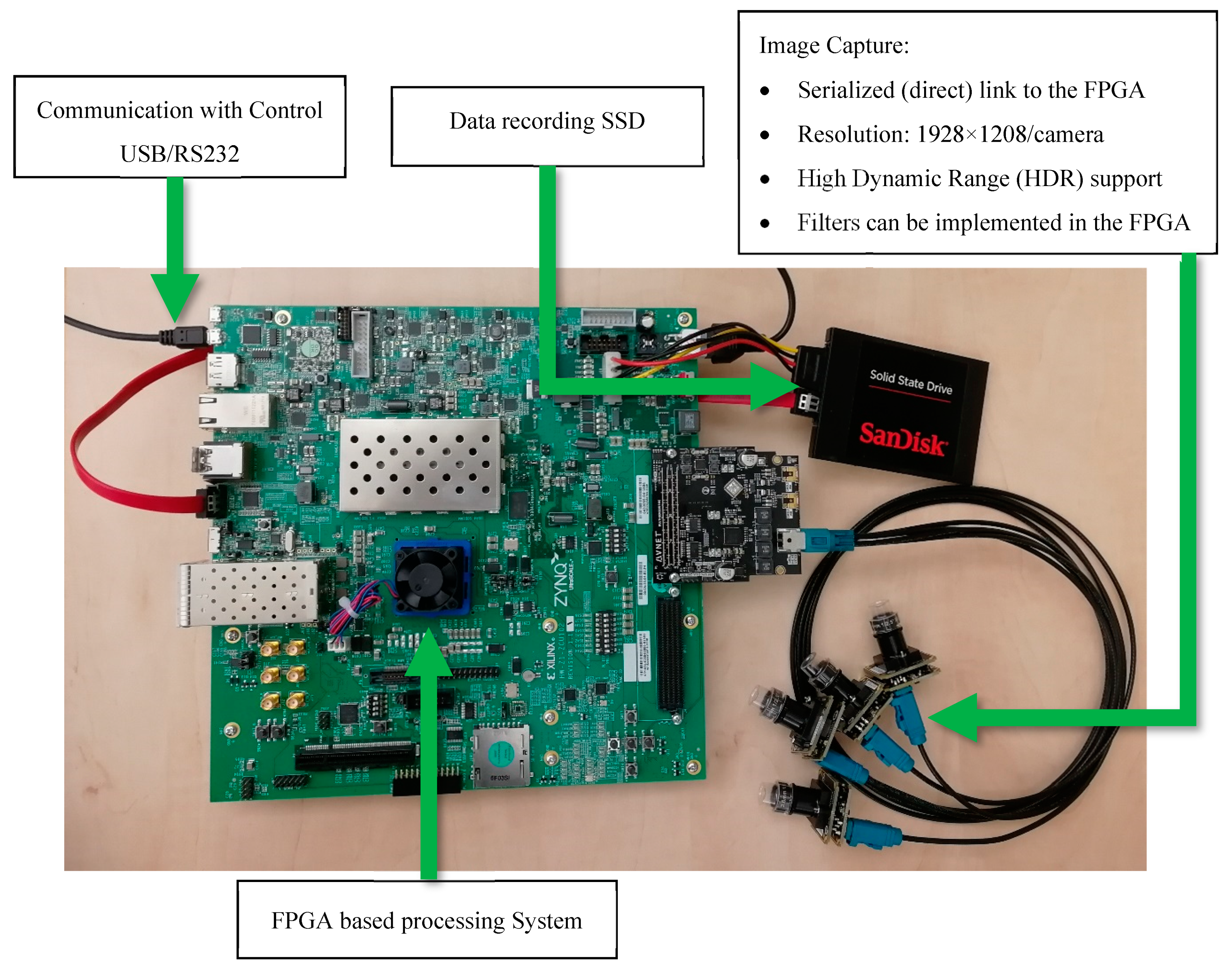
3.2. FPGA-Based Vision System Hardware

A field programmable gate array (FPGA)-based processing system is under development (Figure 9), on which it is possible to test finalized algorithms with more cameras at higher framerates, with lower power consumption compared to the embedded GPU. On the other hand, integration and test of such customized hardware to consider it flight-ready is very tedious, and we can also confirm its capabilities based on offline tests, with real flight data captured by the GPU-based system.

For research flexibility, we use a high-end FPGA Evaluation Board, Xilinx Zynq UltraScale+ Multi-Processor System-on-Chip (MPSoC) ZCU102. It contains various common industry-standard interfaces, such as USB, SATA, PCI-E, HDMI, DisplayPort, Ethernet, QSPI, CAN, I²C, and UART.

For image capturing, an Avnet Quad AR0231AT Camera FMC Bundle set can be used. This contains an AES-FMC-MULTICAM4-G FMC module and four High Dynamic Range (HDR) camera modules, each with an AR0231AT CMOS image sensor (1928 × 1208), and MAX96705 serializer. Due to the flexibility of the system, this can be changed to other image capturing modules/methods, even to USB cameras.

4. FPGA Implementation

In this section, the FPGA implementation of the horizon detection module is presented for distortion-free and distorted images. This circuit is a part of an FPGA-based image processing system for collision avoidance. First, the whole (planned) architecture is briefly introduced, then the details of the realized horizon detection module are given with its power and programmable logic resource need on the FPGA.

4.1. Image Processing System on FPGA

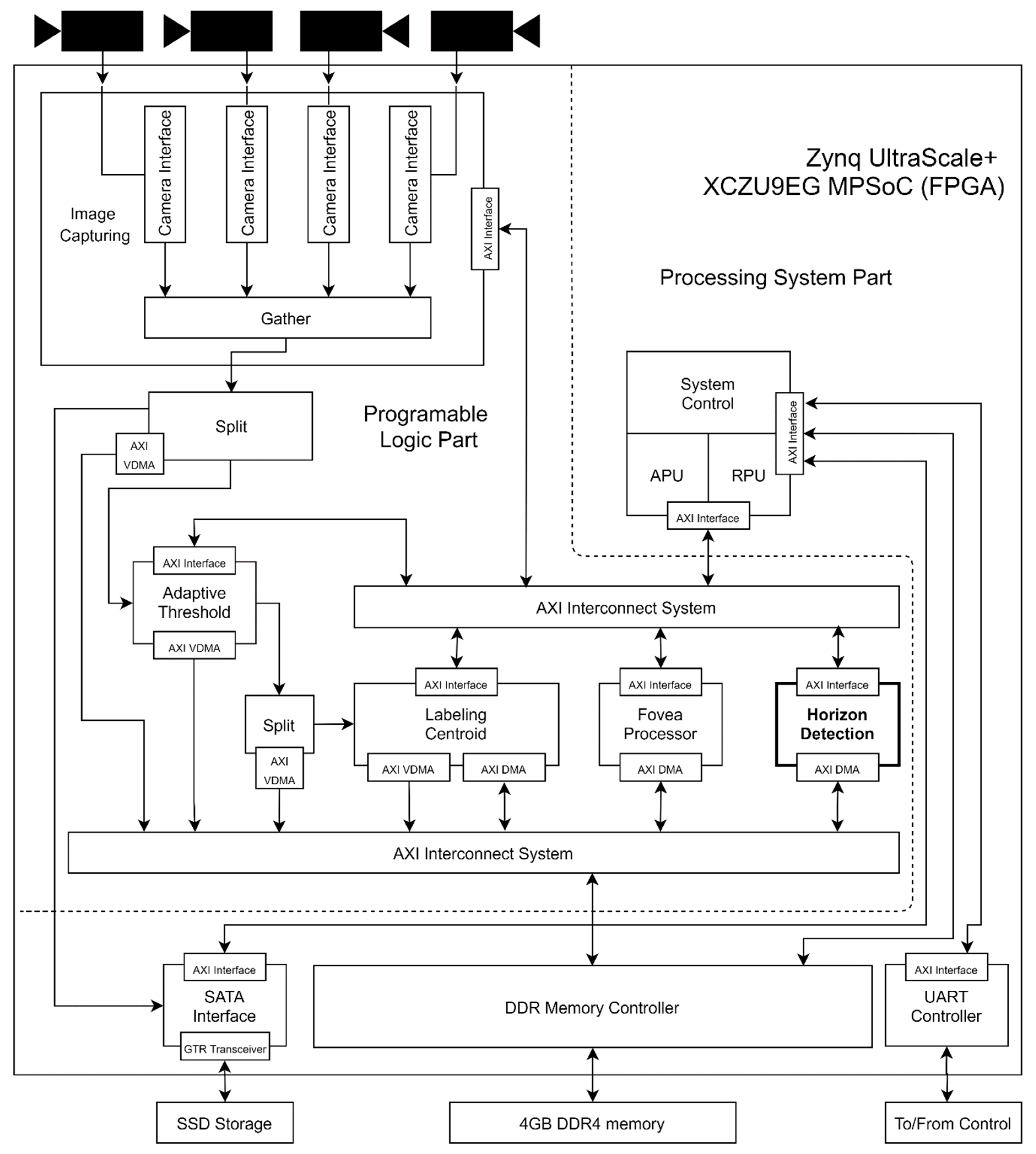
The Zynq UltraScale+ XCZU9EG MPSoC FPGA chip has two main parts. The first is the FPGA Programmable Logic (PL). This contains the programmable circuit elements, such as look up tables (LUT), flip-flops (FF), configurable logic blocks (CLB), block memories (BRAM) and digital signal processing blocks (DSP) that are special arithmetic units designed to execute the most common operations in digital signal processing. The second part is called processing system (PS). Unlike the PL part, this contains fixed functional units, such as a traditional processor system, integrated I/Os and memory controller. PS has an application processing unit (APU) with four Arm Cortex-A53 cores at up to 1.5 GHz. A real-time processing unit (RPU) is also available with two Arm Cortex-R5 cores. There are fixed AXI BUS connections between the PL, PS, and the integrated I/Os.

Figure 10 shows the complete architecture of the SAA vision system. This architecture is based on [22] and not completely ready. In this paper, we introduce the horizon detection module and its role in the complete SAA system.

The PS part is used to control the image processing system. It sets the basic parameters of the different modules, reads their status information, and handles the communication with the control system. Some integrated I/Os are also utilized in this part. Raw image information is stored via the SATA interface. This can work as a black box during flight, and also makes it possible to use previously recorded flight data in offline tests. The DDR memory controller is connected to the onboard 4GB DDR4 memory. The UART controller performs the communication between the AHRS and the image processing system.

The computationally intensive part of the system is placed in the PL part. First, we capture the camera image of each camera and bind them together, making a new extended image. This is piped to three data paths: one to the SSD storage via the SATA interface, one to the memory (the other modules can access the raw image), and the third to the adaptive threshold module.

The input dataflow is examined by an n×n (now it’s 5×5) window looking for high contrast regions, which are marked in a binary image, that is sent to the Labeling-Centroid module and stored in the memory. In the next step, objects are generated from the binary image. In the beginning, every marked region is an object and gets an identification label. If two marked regions are neighbors (to the left, right, up, down, or diagonally), they can be merged into one object. Due to some special shapes, like U, there is a second step in merging. The centroid of every object is calculated and stored.

When a full raw image is stored in the memory, the horizon detection module starts the calculation based on the AHRS data. The module returns the parameters of the horizon line, that can be used by the PS.

When both the horizon detection and the labeling-centroid module have finished, the PS is notified. Based on the current number of objects, the adaptive threshold module is set, as the number of objects on the next image should be between 20 and 30. Based on the horizon line, the PS determines that an object should be further investigated, or it can be dropped (the system detects sky objects only). The Fovea processor classifies the remaining objects, and the PS tracks the objects which were considered as intruders by the Fovea processor. The evasion maneuver is triggered based on the track analysis. For more details about the concept of this FPGA-based SAA image processing system, see [22].

4.2. Horizon Detection Module

In [8], the distortion-free version of the horizon detection was introduced and implemented on an Nvidia Jetson TK1 embedded GPU system. In this paper, we introduce direct handling of radial distortion without undistortion of the whole image, which is also implemented and used in-flight with the TK1 system. Here, we give the FPGA implementations for both the distorted and the distortion-free cases.

The TK1 C/C++ code is slightly modified to suit FPGA architecture design requirements better. High levels synthesis (HLS) tools were used to generate the hardware description language (HDL) sources from the modified C/C++ code. The main advantage of HLS compared to the more general pure HDL way is that the development time is much less, while it still gives low-level optimization possibilities.

4.2.1. Horizon Detection Without Radial Distortion

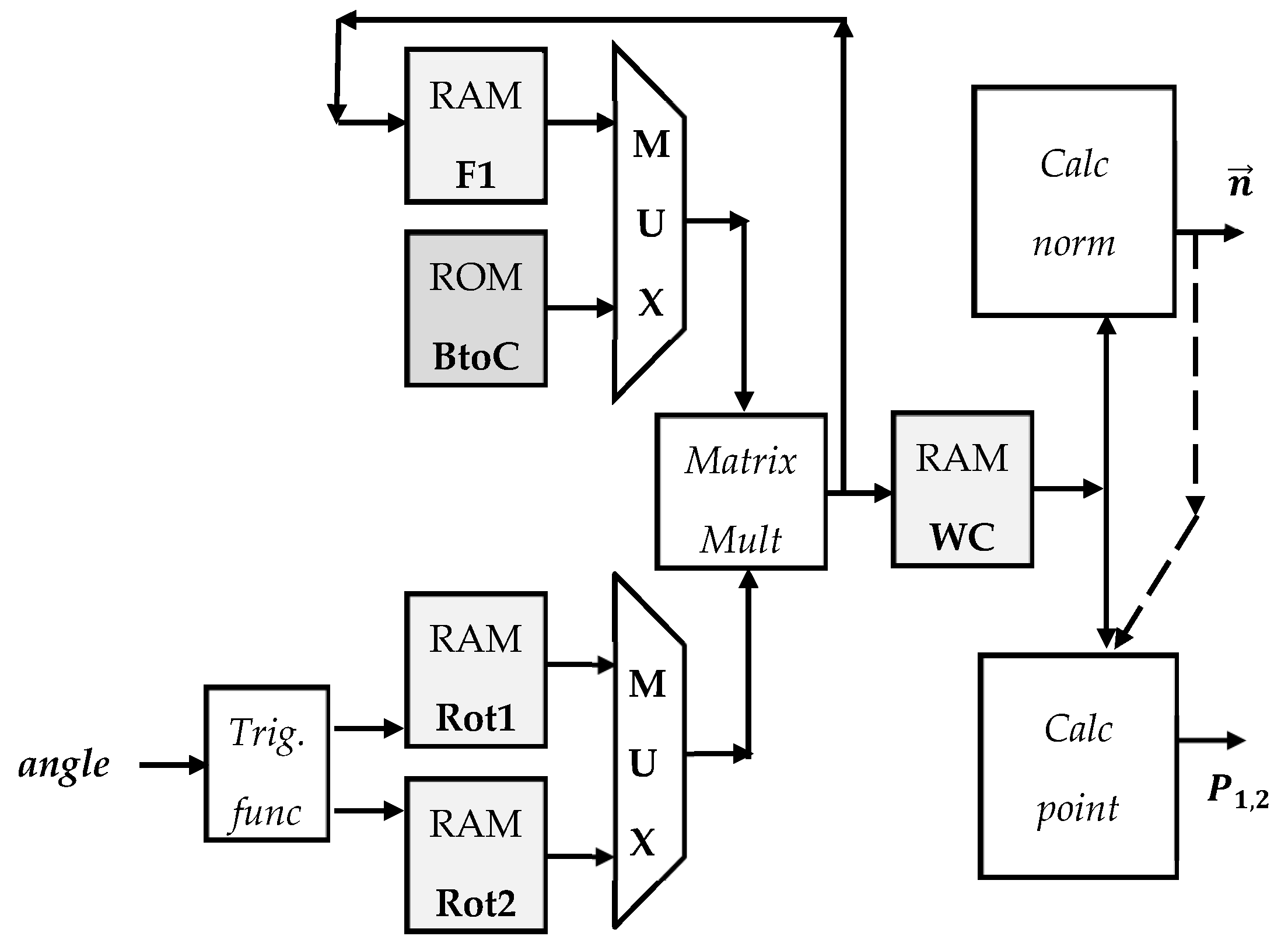
The block diagram of the AHRS-based pre-calculation [8] submodule is shown in Figure 11. First, the trigonometric functions of the Euler angles are calculated. The result is written in Rot1 or Rot2 memory, which works like a ping-pong buffer. In this implementation, when the result is available in one of the memories, the system starts the matrix multiplication. The transformation matrix from the body frame to the camera frame (BtoC) depends on only constants. Thus, it is calculated offline and stored in a ROM. The design is pipelined, therefore during the matrix multiplication, the system calculates another trigonometric function. When the $WC$ matrix, which defines the projection from the world coordinate system to the camera frame, has been calculated, the system writes it to a memory module.

After that, the transformation of the AHRS-horizon parameters, a normal vector (calc norm), and the two points of the line (calc point) occur in parallel. These two (three) values define the pre-calculated horizon line on the image.

The block diagram of the FPGA implementation of the post-calculation (Gradient Sampling) is shown in Figure 12. The endpoints of the pre-calculated horizon are derived from the normal vector and the point from the previous step. The “Case Calc” module is estimating the location of the endpoints on the image. For this estimation, eight regions are distinguished: The four sides and the four corners. This is used as an auxiliary variable for the calculations. It is necessary to check if the horizon line is in the image, based on the endpoints (check). If the endpoints are on the image, the coordinates of the base points (BP) are calculated, and these are stored in a RAM. Otherwise, the “valid” signal will be false, and the following steps are not calculated.

In a cycle of rotations, the base points are rotated in each step with a predefined angle. The values of the trigonometric functions (sin, cos) are calculated for these predefined angles, and they are stored in a ROM (trig). The result of the rotation is stored in RAM RP, and an inner cycle is run for the shift (cycle shift). In cycle shift, only those point pairs are used for the average intensity difference calculation, where both points are in the image. For each run, the result is compared to the best average so far, which is stored in RAM BEST&NV. The normal vector and a point of the line are also stored. The cycles are pipelined to speed up the calculation. In the end, the two endpoints and the normal vector of the horizon are calculated in EP&NV.

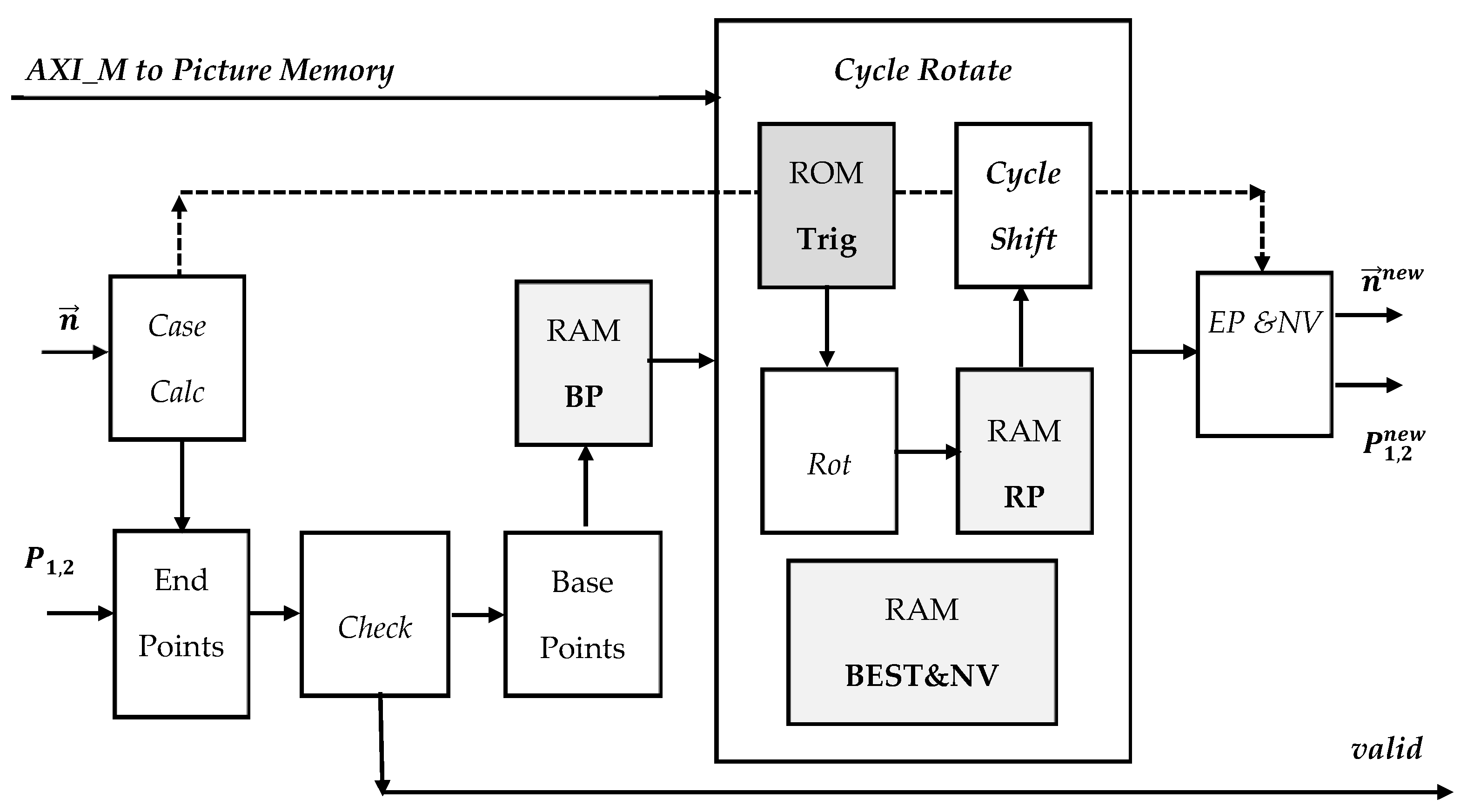
4.2.2. Horizon Detection with Radial Distortion

The pre-calculation submodule is nearly the same as in the distortion-free case. The only difference is that we calculate only one point; the center point, not two.

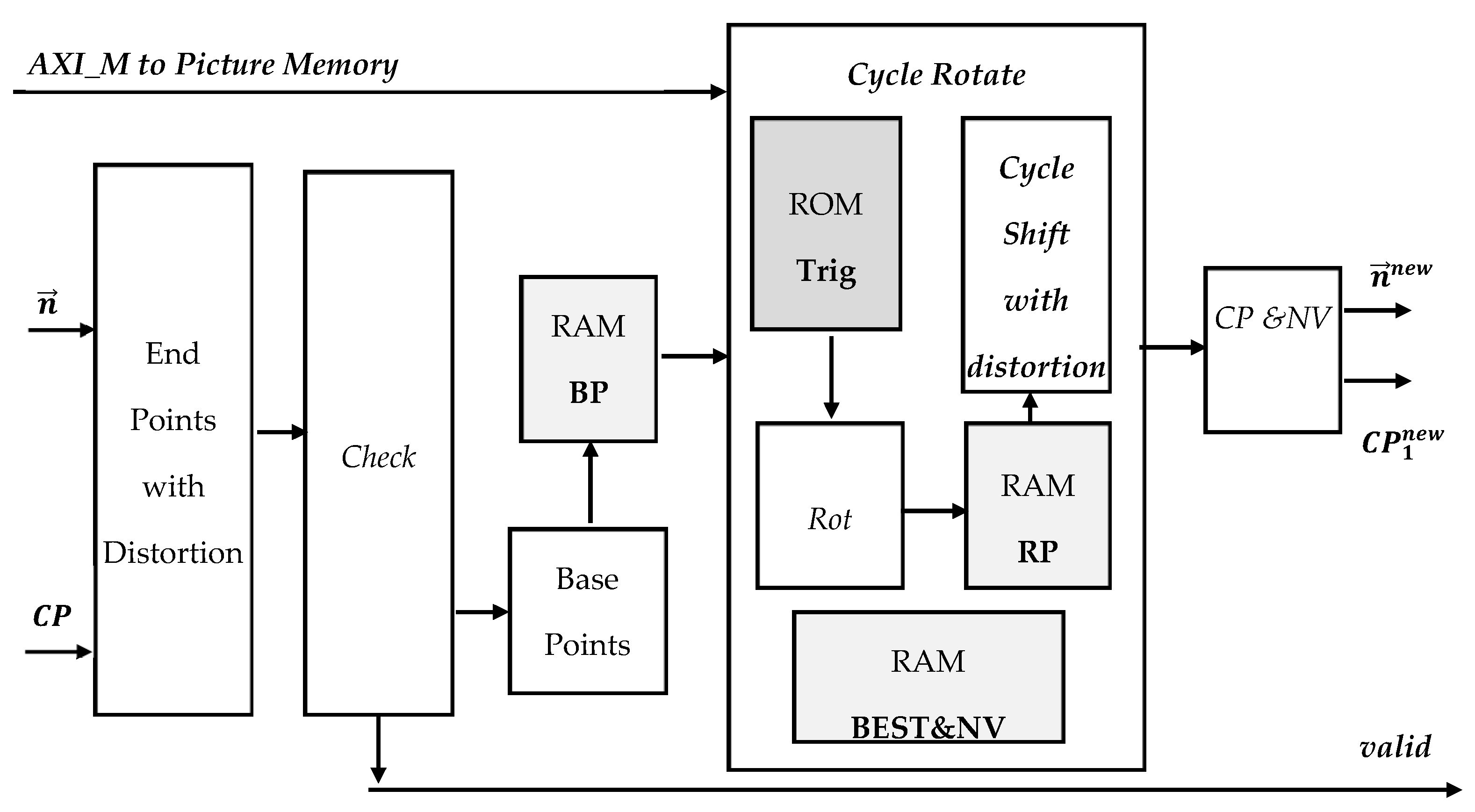
The post-calculation submodule required noticeable modifications. Due to the distortion, it can happen that we have even four intersections with the borders. Of course, in this case, only the left- and the rightmost intersections are used. Therefore, the case calculation block was eliminated, end the endpoint calculation module was extended with the functionality of handling the distortion. The other changes in this submodule were in the cycle shift block. The other functionalities of the blocks remained the same as the distortion-free case. In all shift cycles for every sample point pairs, the distortion is calculated, and the samples are taken from the distorted pixel coordinates. In the end, a normal vector and the center point of the (tuned) horizon are calculated in CP and NV block. The block diagram of the modified post-calculation submodule is shown in Figure 13.

4.2.3. Resource and Power Usage

The two different FPGA modules (with and without radial distortion) were optimized by two different strategies. The first strategy aims for the highest possible clock rate/lowest evaluation time, but keeping the requirement that the total usage of the available resources cannot be greater than 20% (referred to as “Speed” implementation). The second one aims for less resource usage, even suitable for low-cost FPGA-s (referred to as “Area” implementation). Based on HLS technology, the C/C++ source during this process remained the same, and only the optimization directives/pragmas were changed. All implementations use floating-point number representations to have the same numeric properties as the TK1 implementation. However, these results can be further optimized with a fixed-point machine number representation. Execution time mainly depends on the number of sample points (20) of the gradient sampling phase and its search parameters, such as the number of rotation (±15 degree/1 degree step) and shift (±120 pixel/5 pixel step) steps.

The properties of each architecture are shown in

Table 1. The clock frequencies, execution times, and resource usage of different implementation strategies.

	Without Distortion		With Distortion
Optimization Goal	Speed	Area	Speed	Area
Timing
Clock Frequency	~110 MHz	~72 MHz	~100 MHz	~72 MHz
Execution Time	~1.2 mS	~1.8 mS	~1.4 mS	~2 mS
Resource
BRAM_18K	2	2	2	2
DSP48E	70	48	211	75
FF	20,336	14,056	42,624	30,163
LUT	26,698	23,554	49,408	34,744
Resource %
BRAM_18K	~0%	~0%	~0%	~0%
DSP48E	2%	1%	8%	4%
FF	3%	2%	7%	5%
LUT	9%	8%	18%	12%

. Even the resource optimized version (Area) with distortion has 2 mS execution time. The other versions have better results, but are relatively close to this. If we are comparing the speed and area versions, we can see that the resource usage can be reduced, especially when we calculate the distortion. On the other hand, the maximum clock frequency is also decreased. In this (area) case the resource elements (multipliers, adder, and others) are shared between the different blocks. This reduces the number of them, but generates a more complex control flow graph, thus a more complex final state machine that cannot operate at a high clock frequency as the speed implementation. Distorted and distortion-free versions do not have a huge difference in execution time. Distortion handling requires more circuit resources, four times more DSP, and two times more FF and LUT.

The estimated power usage of the whole image processing system is below 5 Watts. It doesn’t matter which horizon detection module is used, and it remains 5 W, because the most power consuming part of the system is the PS, not the PL in which the horizon module lies. More than 80% of the whole usage comes from the PS part. The estimation is based on the Xilinx Vitis/Vivado built-in power consumption estimator.

5. Experimental Results

The performance measurement of the horizon detection algorithm was done off-line, using the in-flight video and sensor data. Three flight video segments were analyzed; two of them consist of 1220 frames, and one of them consists of 1203 frames, which covers 2.5 min for each video considering the 8Hz sampling frequency. Each frame consists of two images; thus, altogether, more than 7000 horizons were evaluated. On each image, the horizon line was annotated by hand. Frames, where the horizon cannot be seen, are skipped from the calculations. There were around 1000 of these images. Tests for the undistorted case (2 videos) and the distorted case (1 video) were run on videos captured at Matyasfold.

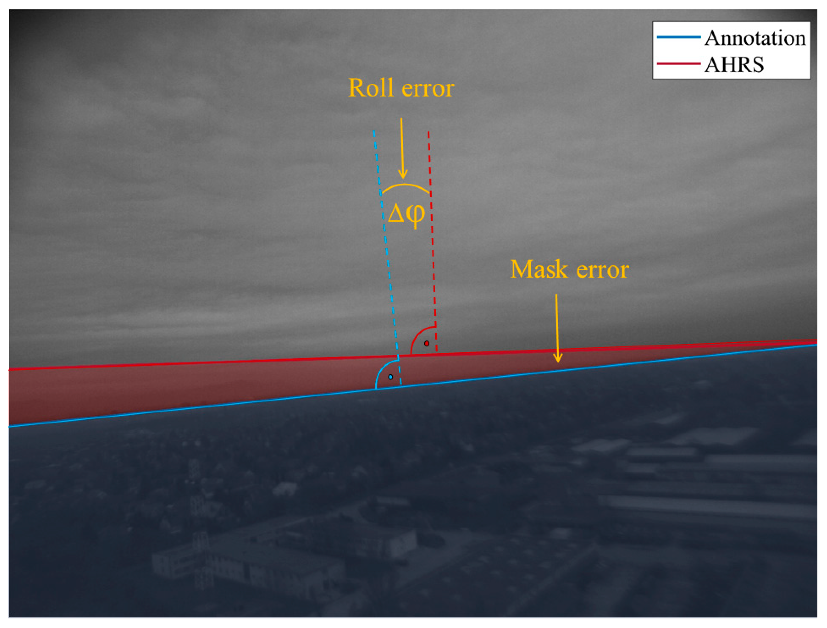
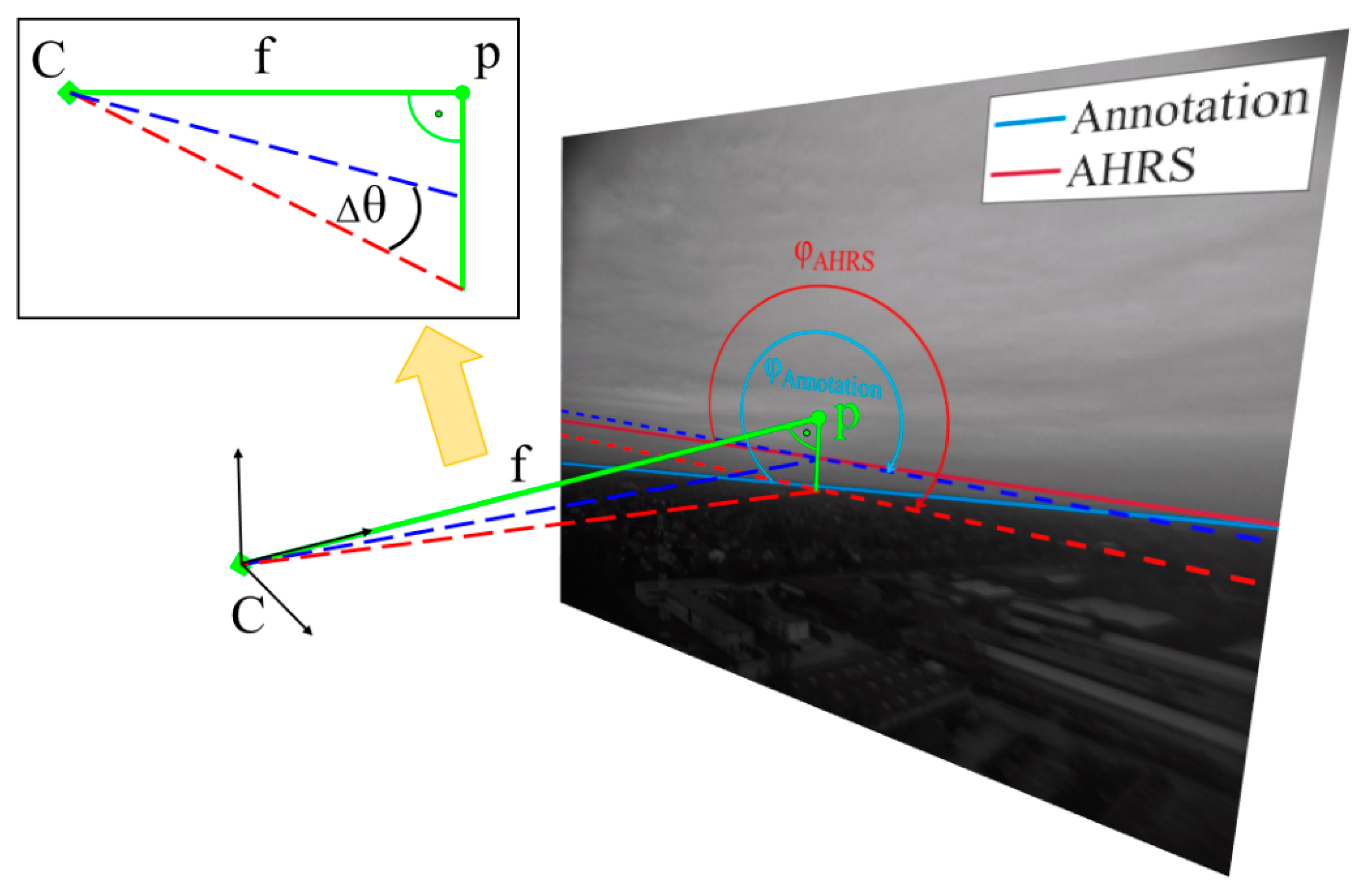
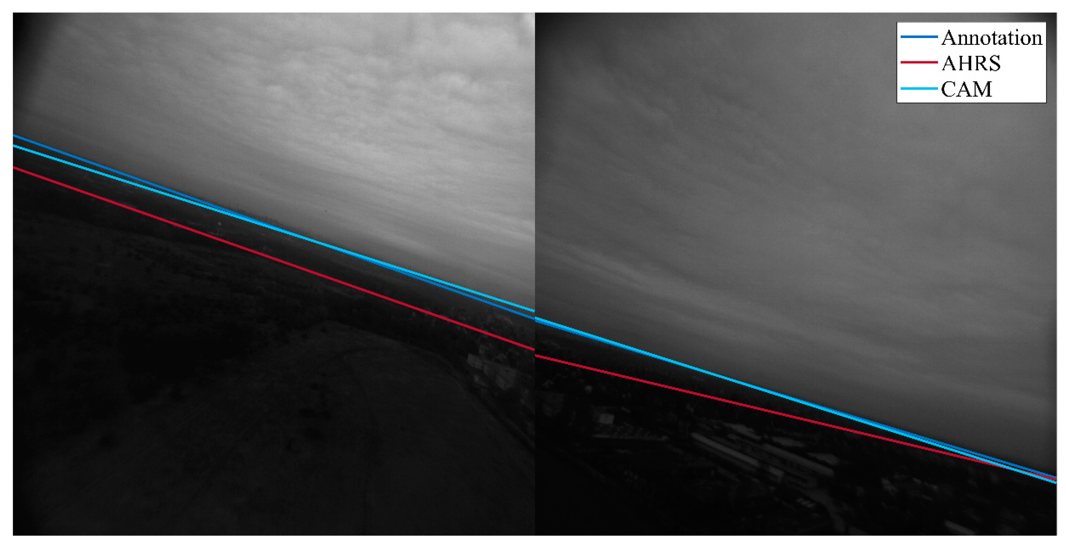
The AHRS and the CAM results were tested against the annotation. Three error measures were calculated to show the performance of the horizon detection: (1) roll angle error (2) pitch angle error (3) sky mask pixel ratio error. The geometric interpretation of these error terms is shown in Figure 14 and Figure 15, and a graphical comparison of the algorithms to the annotation is shown in Figure 16.

AHRS of the Sindy aircraft with its full functionality (Inertial-Magnetic-Barometer—GPS) can provide attitude angles with less than 2-5-degree error. Thus, the horizon candidates of the pre-calculation step are close to the visual horizon in the image as it can be seen in Figure 16. The fine-tuned horizon output is nearly identical to the real visual horizon; only hills and long white urban structures near the horizon can disturb the fit. 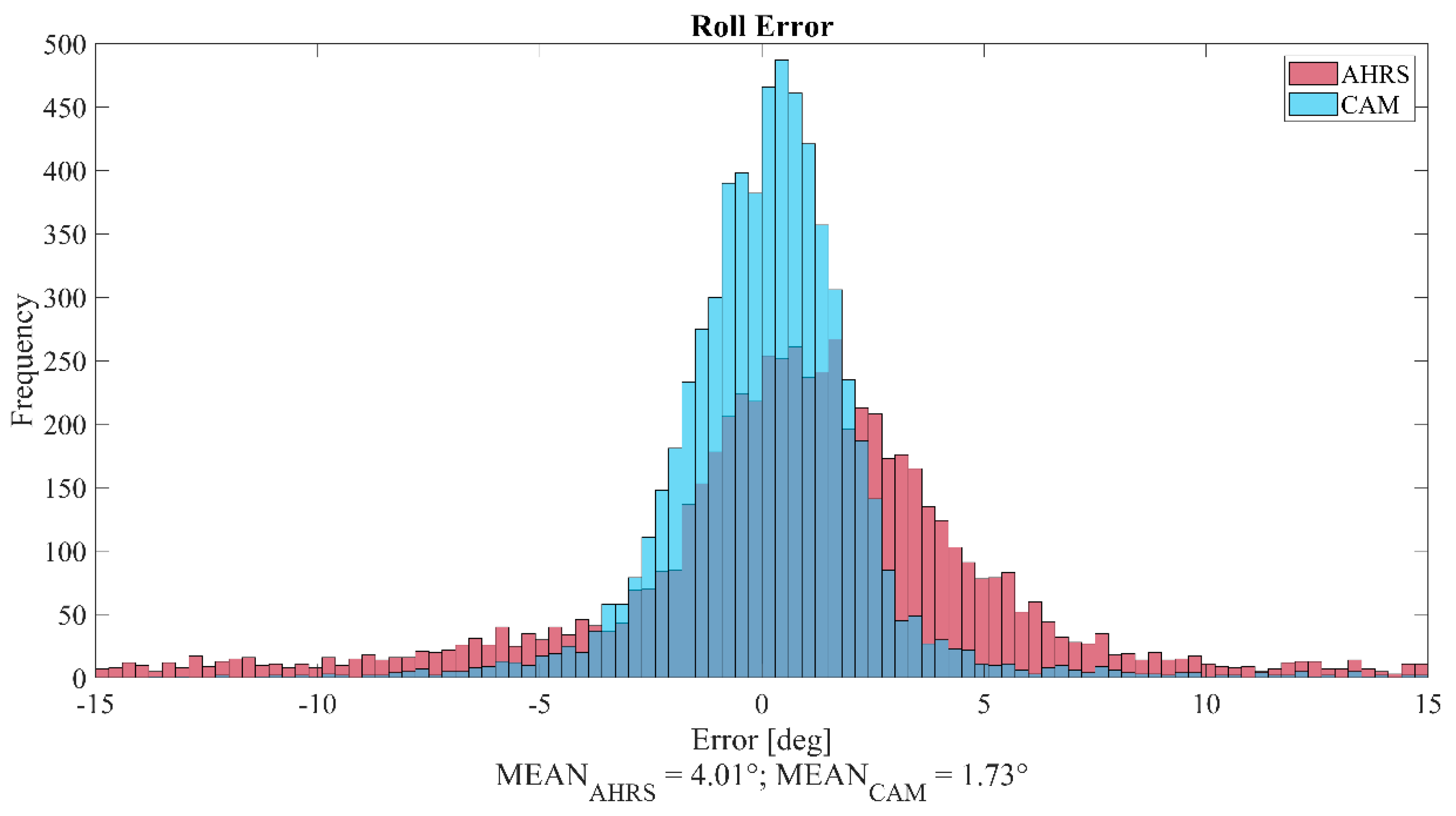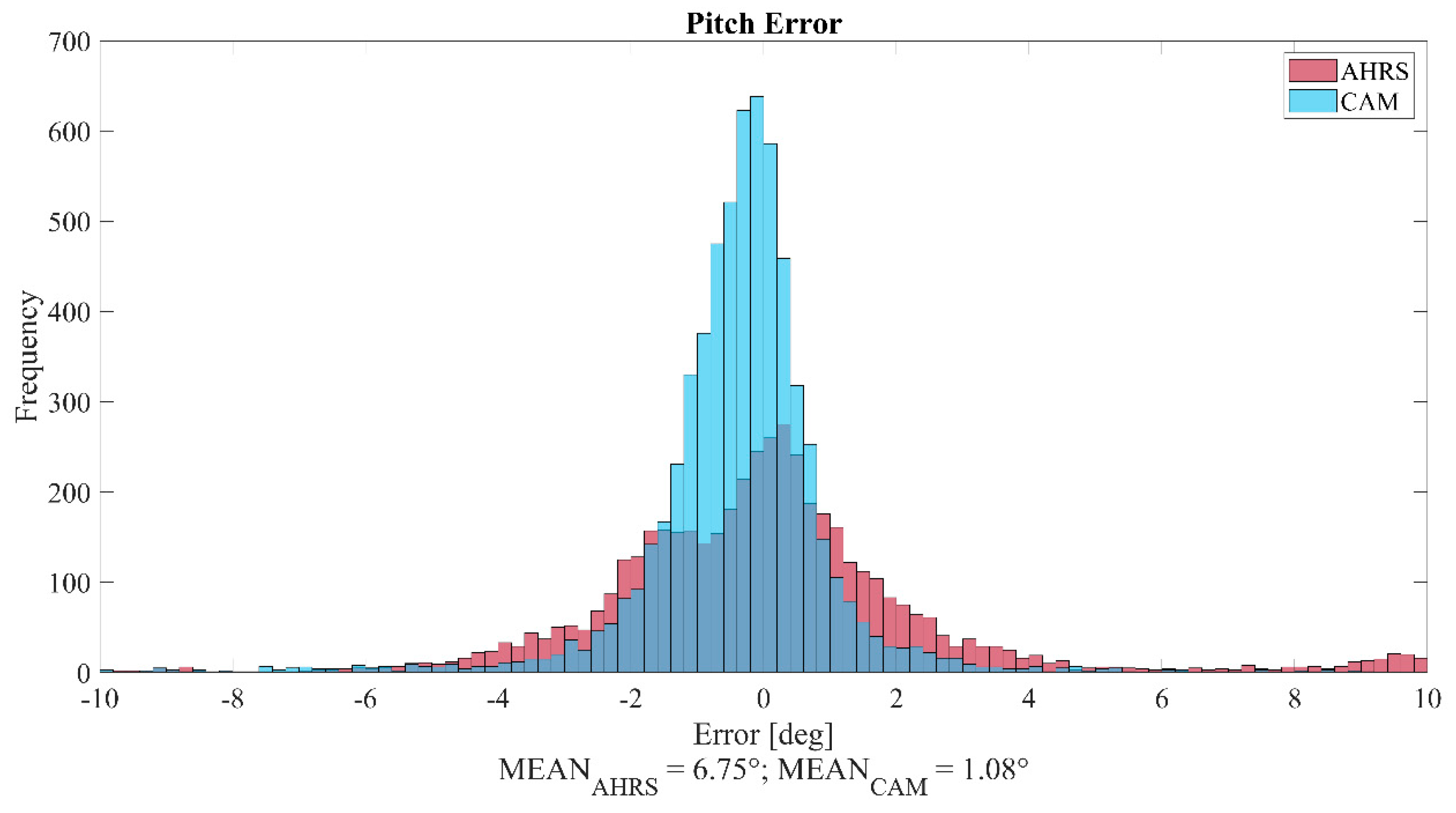Figure 17 presents the effect of the gradient sampling phase, which can improve the AHRS horizon candidates from a 4.01 degree average absolute roll error to 1.73 degrees. We can see even better improvement for the pitch angle in Figure 18; from 6.75 degrees to 1.08 degrees.

The bias of AHRS angles may come from the not ideal plane surface of the Mátyásföld area, and the possible small ~0.5-degree relative calibration error of the camera. With the elimination of this bias, we can still have benefited from the vision-based horizon, thanks to the fine angular resolution of our images compared to other methods that do not utilize the AHRS candidate and run complex sky-ground classification methods in low resolution to find a visual horizon. The real-time implementation of [18] reported a 1.49-degree average pith/roll error, which is close to other slower methods. Obviously, we have not solved the same challenging problem as other horizon detectors, which use only the image. However, we utilized the AHRS, which is always at hand on-board, and reach same performance on radially distorted images without undistortion of the complete image. The number of sample points (20), the number of rotation (+-15 degrees/1 degree resolution) and shift (+-120 pixel/5 pixel resolution) steps can be increased to reach better accuracy and robustness, however, the computational need has linear growth. This setup was suitable for our sky-ground separation application, where the main SAA mission task occupied most of our on-board computational resources.

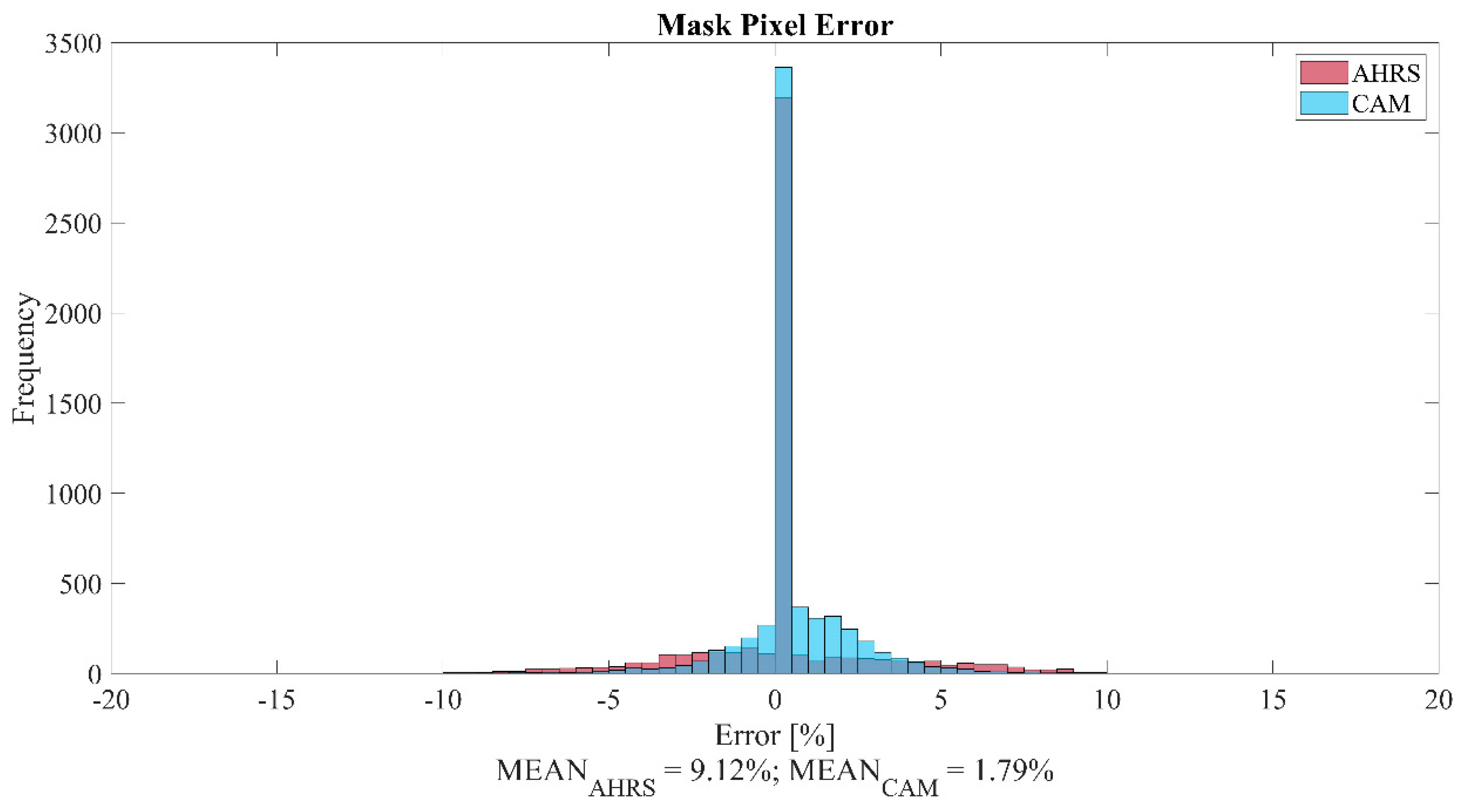
Due to the fact that we use the horizon for sky-ground separation, we also investigate the ground mask pixel error as the percentage of the image (Figure 19). Here, we can see the sum of roll and pitch improvement.

The gradient sampling with native distortion handling was initially implemented on the Nvidia Jetson TK1 embedded GPU and used in several flight tests with the Sindy aircraft. In this article, we gave the FPGA implementation for the horizon detection module to demonstrate that this problem can be solved under 5 W power in 2 mS time.

Table 2. The execution time of different horizon detection algorithms, on the given computer architecture and image size in the distortion-free case.

Algorithm	Computer Architecture	TDP	Camera Resolution (Resolution for Calculation)	Execution Time
Todorovic [12]	Athlon x86 @900 MHz	60 W	640 × 480 (128 × 128)	~600 mS
Ettinger et al. [11]	x86 @900 MHz	~60 W	320 × 240 (80 × 60)	~33 mS
McGee et al. [13]	Pentium III x86 @700 MHz	~24 W	320 × 240	~500 mS
Boroujeni et al. [14]	x86 @2.4 GHz (MATLAB)	~60 W	250 × 150	~2000 mS
Dusha et al. [16]	Pentium IV @3 GHz	84 W	352 × 288	~70 mS
Moore et al. [18]	dual-core PC104 @ 1.5 GHz	~20 W	360 × 180 (80 × 40)	~2 mS
Ours – NVIDIA TK1 [8]	ARM Cortex A15 @ 2.3 GHz	10 W	1280 × 960 (does not depend on resolution)	~5 mS
Ours – FPGA (Zynq UltraScale+ ZCU102)	Custom	<5 W	1928 × 1208 (does not depend on resolution)	~1.2 mS

summarizes some reference algorithms and test platforms. Only [18] is close to the TK1 implementation. However, we have reached better accuracy, with the help of AHRS attitude information. The FPGA module for the distortion-free case can reach 1.2 mS response time with 20 sample points.

Another way to handle distortion is to undistort the full image and then, run the simple horizon algorithm. In the literature, most of the undistortion algorithms consider a region of interest (ROI) and only distort this smaller area instead of the full image [23], which makes it possible to use simpler distortion models in a small part of the scene. In our case, we cannot predefine a ROI. Therefore, these methods are not suitable. In general, the system latency is increased with the full image undistortion time, because the horizon search algorithm can be started only with the fully undistorted image. Even if a fix-point number-representation is used, it takes around 20 mS on a full HD image (based on [24]). In our solution, the difference between the distorted and the undistorted version is only 0.2 mS (more FPGA circuit resources are consumed).

6. Conclusions

This paper presents a light-weight gradient sampling-based visual horizon detection for radially distorted images. Operating in planar environments where the horizon is a visible feature, the method explores the neighborhood of a horizon candidate, which is defined by the yaw pitch roll angles of the attitude heading reference system (AHRS), which is a piece of common equipment on a UAS. Vision-only methods are computationally more expensive, thus they are performed in low resolution and require radial undistortion of the image. In our case, the complete undistortion of the image is not necessary; only a few numbers of sample points should be transformed. The computational complexity of the method is independent from the image size, thus down sampling is not necessary. The original fine resolution image can provide better angular accuracy for the horizon detection.

The exact form of the distorted horizon is derived, which is a fifth order polynomial, and makes it possible to have the best quality representation if it is needed. The gradient sampling algorithm can efficiently improve even good quality AHRS data, based on the visual horizon. FPGA implementation is also given for the horizon detection, which demonstrates that the distortion handling can be performed with minimal time need (1.2 ms), if we add some extra circuit resources to the module. This realization is the fastest known vision-based horizon detector. The time complexity is defined by the number of sample points, rotation and shift steps. Our on-board setup has 1.7 degree roll and 1 degree pitch average absolute error, which is suitable for most applications and better than the vision-only real-time methods.

If complete undistortion of the whole image is not necessary for the main mission of the UAV, the horizon detection does not require it. A simple search around the AHRS-based horizon can reach high-quality attitude or sky-ground image masks.

References

- Mogili, U.R.; Deepak, B.B.V.L. Review on application of drone systems in precision agriculture. Procedia Comput. Sci. 2018, 133, 502–509. [Google Scholar] [CrossRef]
- Zsedrovits, T.; Peter, P.; Bauer, P.; Pencz, B.J.M.; Hiba, A.; Gozse, I.; Kisantal, M.; Nemeth, M.; Nagy, Z.; Vanek, B.; et al. Onboard visual sense and avoid system for small aircraft. IEEE Aerosp. Electron. Syst. Mag. 2016, 31, 18–27. [Google Scholar] [CrossRef]
- Fasano, G.; Accardo, D.; Tirri, A.E.; Moccia, A.; De Lellis, E.E. Morphological filtering and target tracking for vision-based UAS sense and avoid. In Proceedings of the 2014 International Conference on Unmanned Aircraft Systems (ICUAS), Orlando, FL, USA, 27–30 May 2014; pp. 430–440. [Google Scholar]
- Molloy, T.L.; Ford, J.J.; Mejias, L. Detection of aircraft below the horizon for vision-based detect and avoid in unmanned aircraft systems. J. Field Robot. 2017, 34, 1378–1391. [Google Scholar] [CrossRef]
- Gleason, S.; Gebre-Egziabher, D. GNSS Applications and Methods; Artech House: Washington, DC, USA, 2009. [Google Scholar]
- Bauer, P.; Bokor, J. Multi-mode extended Kalman filter for aircraft attitude estimation. IFAC Proc. Vol. 2011, 44, 7244–7249. [Google Scholar] [CrossRef]
- Cornall, T.D.; Egan, G.K. Measuring Horizon Angle from Video on a Small Unmanned Air Vehicle. Auton. Robots 2004, 339–344. [Google Scholar]
- Hiba, A.; Zsedrovits, T.; Bauer, P.; Zarandy, A. Fast horizon detection for airborne visual systems. In Proceedings of the 2016 International Conference on Unmanned Aircraft Systems (ICUAS), Arlington, VA, USA, 7–10 June 2016; pp. 886–891. [Google Scholar]
- Zsedrovits, T.; Bauer, P.; Hiba, A.; Nemeth, M.; Pencz, B.J.M.; Zarandy, A.; Vanek, B.; Bokor, J. Performance Analysis of Camera Rotation Estimation Algorithms in Multi-Sensor Fusion for Unmanned Aircraft Attitude Estimation. J. Intell. Robot. Syst. 2016, 84, 759–777. [Google Scholar] [CrossRef]
- Gibert, V.; Burlion, L.; Chriette, A.; Boada, J.; Plestan, F. Nonlinear observers in vision system: Application to civil aircraft landing. In Proceedings of the 2015 European Control Conference (ECC), Linz, Austria, 15–17 July 2015; pp. 1818–1823. [Google Scholar]
- Ettinger, S.M.; Nechyba, M.C.; Ifju, P.G.; Waszak, M. Towards flight autonomy: Vision-based horizon detection for micro air vehicles. In Proceedings of the Florida Conference on Recent Advances in Robotics, Melbourne, FL, USA, 14–16 May 2002. [Google Scholar]
- Todorovic, S. Statistical Modeling and Segmentation of Sky/Ground Images. Master’s Thesis, University of Florida, Gainesville, FL, USA, 2002. [Google Scholar]
- McGee, T.G.; Sengupta, R.; Hedrick, K. Obstacle Detection for Small Autonomous Aircraft Using Sky Segmentation. In Proceedings of the 2005 IEEE International Conference on Robotics and Automation, Barcelona, Spain, 18–22 April 2005; pp. 4679–4684. [Google Scholar]
- Boroujeni, N.S.; Etemad, S.A.; Whitehead, A. Robust horizon detection using segmentation for UAV applications. In Proceedings of the 9th Conference on Computer and Robot Vision, Toronto, ON, Canada, 28–30 May 2012; pp. 346–352. [Google Scholar]
- Bauer, P.; Bokor, J. Development and hardware-in-the-loop testing of an Extended Kalman Filter for attitude estimation. In Proceedings of the 11th IEEE International Symposium on Computational Intelligence and Informatics (CINTI), Budapest, Hungary, 18–20 November 2010; pp. 57–62. [Google Scholar]
- Dusha, D.; Boles, W.; Walker, R. Fixed-Wing Attitude Estimation Using Computer Vision Based Horizon Detection; QUT ePrints: Queensland, Australia, 2007; pp. 1–19. [Google Scholar]
- Shen, Y.F.; Krusienski, D.; Li, J.; Rahman, Z. A Hierarchical Horizon Detection Algorithm. IEEE Geosci. Remote Sens. Lett. 2013, 10, 111–114. [Google Scholar] [CrossRef]
- Moore, R.J.; Thurrowgood, S.; Bland, D.; Soccol, D.; Srinivasan, M.V. A fast and adaptive method for estimating UAV attitude from the visual horizon. In Proceedings of the 2011 IEEE/RSJ International Conference on Intelligent Robots and Systems, San Francisco, CA, USA, 25–30 September 2011; pp. 4935–4940. [Google Scholar]
- Hartley, R.; Zisserman, A. Multiple View Geometry in Computer Vision; Cambridge University Press: Cambridge, UK, 2004; ISBN 0521540518. [Google Scholar]
- Zhang, Z. A flexible new technique for camera calibration. IEEE Trans. Pattern Anal. Mach. Intell. 2000, 22, 1330–1334. [Google Scholar] [CrossRef]
- Vanek, B.; Bauer, P.; Gozse, I.; Lukatsi, M.; Reti, I.; Bokor, J. Safety Critical Platform for Mini UAS Insertion into the Common Airspace. In Proceedings of the AIAA Guidance, Navigation, and Control Conference, American Institute of Aeronautics and Astronautics, Reston, VA, USA, 13–17 January 2014; pp. 1–13. [Google Scholar]
- Zarándy, A.; Nemeth, M.; Nagy, Z.; Kiss, A.; Sántha, L.M.; Zsedrovits, T. A real-time multi-camera vision system for UAV collision warning and navigation. J. Real-Time Image Process. 2016, 12, 709–724. [Google Scholar] [CrossRef]
- Jakub, C.; Henryk, B.; Kamil, G.; Przemysław, S. A Fisheye Distortion Correction Algorithm Optimized for Hardware Implementations. In Proceedings of the 21st International Conference “Mixed Design of Integrated Circuits & Systems”, Lublin, Poland, 19–21 June 2014. [Google Scholar]
- Daloukas, K.; Antonopoulos, C.; Bellas, N.; Chai, S. Fisheye lens distortion correction on multicore and hardware accelerator platforms. In Proceedings of the IEEE International Symposium on Parallel Distributed Processing, Atlanta, GA, USA, 19–23 April 2010; pp. 1–10. [Google Scholar]
Figure 1.
Blue aircraft with a camera on its wing. From the North-East-Down (NED) reference world coordinate system, we can derive the aircraft body frame NED (center of mass origin) and the camera frame NED (camera focal point origin) coordinate systems. S is a North unit vector in a word reference frame, which is parallel to the ground surface.
Figure 2.
Horizon line candidate with the test point sets under (L—red) and above it (H—green).
Figure 3.
Radially distorted lines in images taken by GoPro Hero4. Left: Distorted curves for borders of a chessboard plane. White color indicates the original straight line fractions, mostly covered by the blue, the corresponding radially distorted curves. Right: Curve of the horizon.
Figure 4.
The blue line represents the pre-calculated straight horizon with endpoints P1 and P2. Red crosses and the black curve represent the distorted version of the straight line.
Figure 5.
Block diagram of the horizon detection method. Camera calibration gives constants which should be defined only once. Gradient sampling method can consider radial distortion, with minimal overhead compared to the distortion-free version in [
8].
Figure 6.
The blue dotted curve represents the pre-calculated horizon. Post-calculated horizon curve is formed by line segments between the green points. The effect of the white urban area under the hills can be seen on the right.
Figure 7.
The blue dotted curve represents the pre-calculated horizon. The post-calculated horizon curve is formed by line segments between the green points. The small distortion error at the bottom corner can be seen on the left.
Figure 8.
Sindy aircraft with the mounted Nvidia TK1-based visual SAA system.
Figure 9.
FPGA-based experimental system.
Figure 10.
Block diagram of the FPGA based image processing system for SAA.
Figure 11.
Pre-calculation block diagram. Blocks: F1: temporary memory for matrix multiplication. BtoC: Body frame to Camera Frame transformation matrix. Rot1, Rot2: Ping-pong buffer for trigonometric functions. WC: World to Camera frame transformation matrix.
Figure 12.
Post-calculation (gradient sampling) block diagram without radial distortion. Blocks: BP: Base point storage memory. Trig: Values of trigonometric functions used in rotations. Rot: Rotation calculation. RP: temporary storage for rotated points. BEST&NV: Temporarily stores the parameters of the best founded horizon line. EP&NV: Endpoints and normal vector calculation.
Figure 13.
Post-calculation (gradient sampling) block diagram with radial distortion. Blocks: BP: Base point storage memory. Trig: Values of trigonometric functions used in rotations. Rot: Rotation calculation. RP: temporary storage for rotated points. BEST&NV: Temporarily stores the parameters of the best founded horizon line. CP&NV: Center point and normal vector calculation.
Figure 14.
Roll and mask error definitions.
Figure 15.
Pitch error definition. If the result is rotated around the image center by the roll, then the intersections of the horizons with the perpendicular line which goes through the center can give the pitch angle. We consider the vectors pointing from the 3D focal point of the camera.
Figure 16.
AHRS-based initial horizon candidate (red) the ground truth (blue) and the nearly identical final output of the gradient sampling (cyan).
Figure 17.
Roll error distributions of AHRS-only and the vision-based improvement on the real flight test data, with the average errors.
Figure 18.
Figure 19.
Pixel percentage error of ground masks for AHRS-only and the vision-based improvement on the real flight test data, with the average errors.