Short Circuit Characteristics of PEM Fuel Cells for Grid Integration Applications

Abstract

The reduction of greenhouse gas and pollutant emissions is a major issue in modern society. Therefore, environmentally friendly technologies like fuel cells should replace conventional energy generation plants. Today, fuel cells are used in households for CHP (combined heat and power) applications, for emergency power supply in many stationary applications and for the power supply of cars, buses and ships and emergency power supply of aircrafts. A significant challenge is the optimal electrical grid integration and selection of the appropriate grid protection mechanism for fuel cell applications. For this, the short circuit capability and behavior needs to be known. This paper gives a mathematical estimation of the short circuit behavior of fuel cells. Five main transient and dynamic phenomena are investigated. The impact of the main transient effect for the provision of additional short circuit energy is simulated, and the simulation is experimentally validated. For this purpose, a 25 $\mathrm{c}$$\mathrm{m}$${}^2$ single cell consisting of a Nafion^TM 212 membrane and carbon cloth electrodes with a catalyst loading of $0.5$ $\mathrm{m}$$\mathrm{g}$/$\mathrm{c}$$\mathrm{m}$${}^2$ Pt is analyzed. The magnitude of the transient short circuit current depends on the operating point right before the short circuit occurs, whereas the stationary short circuit current of fuel cells is invariably about twice the operational current. Based on these results, a novel fuel cell model for the estimation of the short circuit behavior is proposed.

1. Introduction

Proton Exchange Membrane (PEM) fuel cells present a promising alternative to conventional power sources in mobile and stationary applications [1,2,3,4,5]. However, optimal grid integration of fuel cell systems is still under investigation; for instance, the limited short circuit capacity of fuel cells to trigger conventional protection systems. This is critical for safe operation, especially in systems with units generating only a limited short circuit current, where an estimate of the available short circuit current is required to dimension a suitable protection system [6]. Due to the good applicability with a fast load response, fuel flexibility, high efficiency and modular production, this technology is going to be largely used in decentralized/virtual power plants [7,8,9,10] or in the transportation system [11,12,13,14,15]. On-board power supplies already experience difficulties similar to a future energy system based on renewable energies and with less conventional generating units regarding the short circuit current capability. An exemplary application is a fuel cell system as a replacement of the kerosene gas turbine, Auxiliary Power Unit (APU), in the rear of an aircraft.

For several years, aircraft manufacturers pursued the implementation of the More Electric Aircraft (MEA) concept. Within this concept, hydraulic and pneumatic systems should be substituted by electrical ones [16,17]. A Multi Functional Fuel Cell System (MFFCS) could increase the efficiency of an aircraft. The application of a fuel cell system as an APU has many advantages [5]:

• Noise reduction,
• Reduction of ground support,
• Emission reduction,
• Water generation,
• Replacement of the Ram Air Turbine (RAT).

However, the optimal integration of an MFFCS in a modern aircraft is a major challenge and needs to be further optimized. This research is focused on the integration of a PEM fuel cell system. Compared to other fuel cell types, this type has a better dynamic characteristic and a higher power density [18]. Both qualities are essential to developing a fuel cell based APU in an aircraft. Other than the traditional APU generator, the MFFCS delivers a direct current. The value of the output voltage of the fuel cell depends on the connected loads. Due to the increasing number of electrical consumers, the voltage level in a modern aircraft could also be increased up to High-Voltage DC (HVDC) 540 ${\mathrm{V}}_{\mathrm{DC}}$ ($\pm 270{\mathrm{V}}_{\mathrm{DC}}$) [19]. The main benefit of the new higher voltage is a decrease in cable weight as a result of the reduced current flow while transmitting the same electrical power. DC/DC converters can be used to transform the variable fuel cell output voltage to the HVDC level [4,20,21].

Currently, the grid protection from the conventional APU generator to the Primary Electrical Power Distribution Center (PEPDC) is based on the overcurrent time protection. This protection mechanism requires a high amount of additional short circuit current capability to detect and isolate an electrical fault, for example, a short circuit. It works reliably for the application of a conventional generator. During the ground phase, when the turbines are shut down, the fuel cell system is the only power source that supplies the electrical aircraft grid in a modern aircraft. When an electrical fault occurs on the isolated aircraft grid, a fuel cell system has to deliver the same short circuit current capability as a conventional generator.

This paper deals with a short circuit current flow estimation for fuel cell systems. In Section 2, a mathematical description to estimate the fuel cell short circuit is presented. Section 3 shows the experimental validation of the deliverable short circuit using a single PEM fuel cell. Based on the simulation and the experimental results, an alternative model for the estimation of the short circuit behavior is given in Section 4. Finally, Section 5 presents a conclusion.

2. Short Circuit Behavior of a Fuel Cell

In order to design a sufficient electrical grid protection mechanism, this chapter deals with the short circuit current capability of fuel cell systems. Therefore, oxygen availability and the transient and dynamic phenomena of a fuel cell system are investigated in more detail. The impact on the provision of an additional short circuit current is simulated.

2.1. Impact of Oxygen Availability on Short Circuit Behavior

For the investigated system, the fuel cell is supplied with hydrogen (H${}_2$) and oxygen (O${}_2$) at ambient pressure. The oxygen is taken from the environmental air [22,23]. Excess air is required to ensure the provision of enough oxygen for the reaction and to remove product water at the cathode. The oxygen excess ratio ${\lambda }_{{\mathrm{O}}_2}$ (Equation (1)) describes the ratio between the actual oxygen mass flow and the required oxygen mass flow for the reaction:

$${\lambda }_{{\mathrm{O}}_2}={\displaystyle \frac{{\dot{m}}_{{\mathrm{O}}_2\mathrm{actual}}}{{\dot{m}}_{{\mathrm{O}}_2\mathrm{required}}}}$$

(1)

Following the thermodynamics of the reaction, the fuel cell will provide the respective current $I_{\mathrm{FC}}$ proportional to the consumed oxygen mass flow, which in turn is proportional to the hydrogen mass flow ${\displaystyle \frac{\mathrm{d}{N}_{{\mathrm{H}}_2}}{\mathrm{d}t}}$ consumed, see Equation (2). Here, F is the Faraday constant (96,485 C/mol), and n is the number of electrons consumed.

$$I_{\mathrm{FC}}=n·F·{\displaystyle \frac{\mathrm{d}{N}_{{\mathrm{H}}_2}}{\mathrm{d}t}}$$

(2)

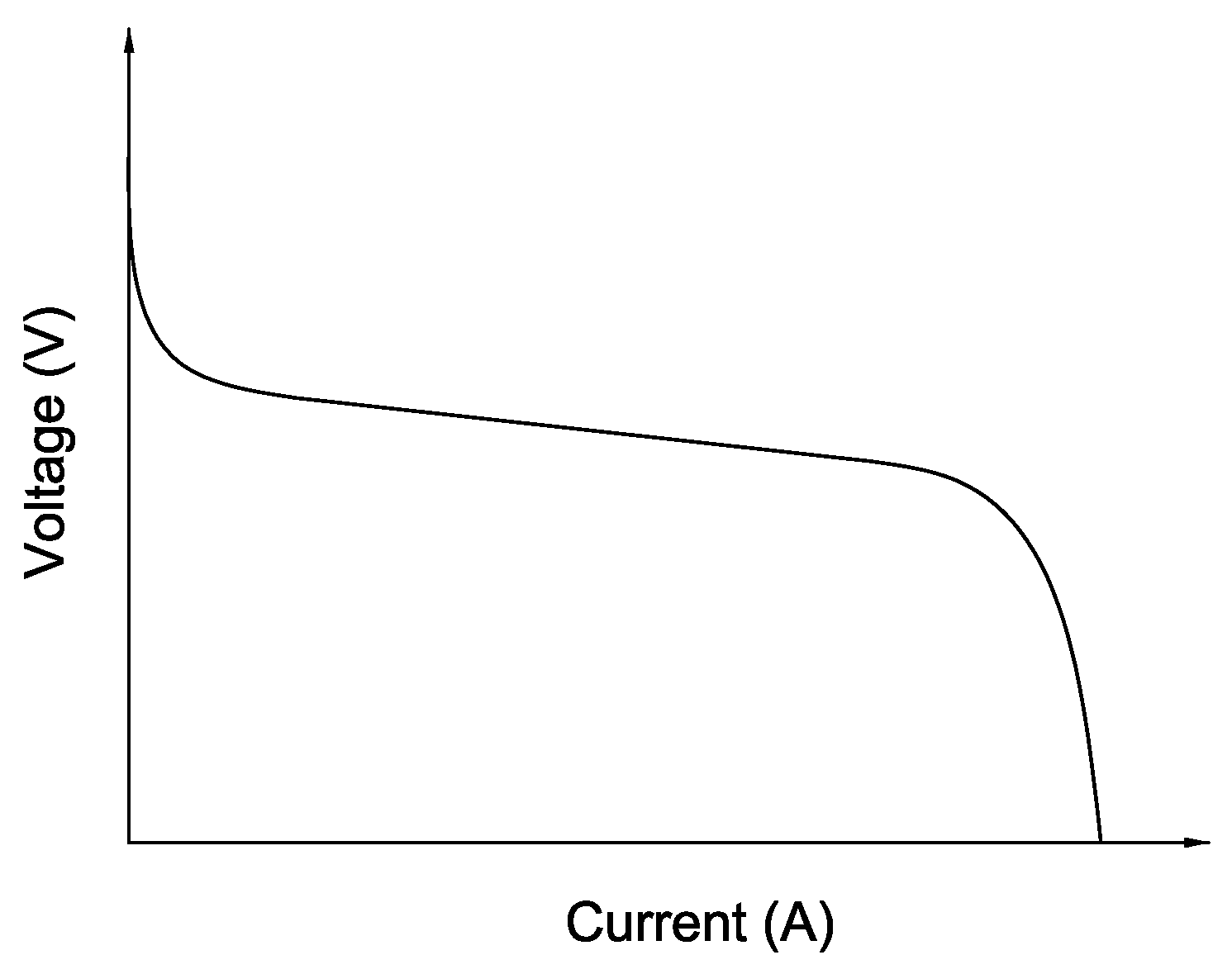
When a short circuit occurs, the voltage drops to nearly zero. Figure 1 shows a typical polarization curve of a fuel cell system. Voltage drops with increasing fuel cell current. It becomes apparent that the fuel cell system delivers the highest amount of electrical current if the voltage drops to zero.

This result is obtained only if there are enough additional oxygen molecules available on the cathode. Due to the complex and relatively long gas channels and the consumption of oxygen, the oxygen partial pressure distribution across the entire cell area is not homogeneous. This results in an increased reaction rate at the inlet and an oxygen starvation near the outlet. For this reason, the oxygen excess ratio ${\lambda }_{{\mathrm{O}}_2}$ is always set greater than one. This ensures a homogenization of the reaction rate over the entire active cell area. Thus, the fuel cell system is operated with a high ${\lambda }_{{\mathrm{O}}_2}$ value. In the case of an electrical short circuit, many reactions take place very quickly. Since the reacting hydrogen is proportional to the amount of the electrical current, a much higher current flow as the nominal current can be provided.

2.2. The Main Transient and Dynamic Effects

Five main transient and dynamic phenomena have been identified in the PEM fuel cell. Figure 2 illustrates these effects with respect to the described time scales. The slowest effect is the stack temperature, which has a time constant in the range of minutes. The second effect is the membrane hydration profile with a transient phase of about 10 s. The third sequence is the reactant flow with a transient phase of about 5 s. The time for the gas diffusion reaction is in the range of some hundreds of milliseconds to 1 s. However, the fastest phenomenon is the double layer charging effect, which is in the range of 1 ms to some tens of milliseconds [24]. All of these transient and dynamic phenomena will affect the output voltage and current of a fuel cell system in non-steady-state operation. Due to the different time scales, only the two fastest phenomena are of interest for the investigated short circuit capability.

2.3. The Electrochemical Double Layer

The double layer charging effect is one important phenomenon to describe the transient behavior of fuel cell stacks. Through the gathering of electrons (${\mathrm{e}}^{-}$) and protons (${\mathrm{H}}^{+}$) at the electrode–electrolyte interface, a voltage drop exists. 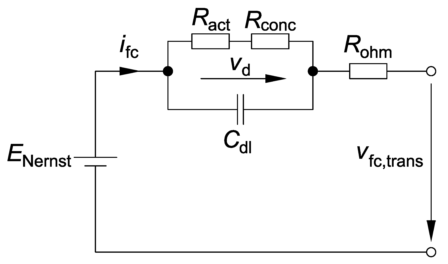This effect is known as the electrochemical double layer, which stores electrical energy and behaves like a capacitor on both electrodes [25]. For this reason, the behavior of the fuel cell due to the electrochemical double layer at a short circuit is calculated and simulated in MATLAB/Simulink. Figure 3 presents an equivalent electrical circuit, which is typically used to simulate transient fuel cell voltage behavior [26].

In Figure 3, $C_{\mathrm{dl}}$ represents the capacitor, which describes the double layer capacity. $R_{\mathrm{ohm}}$, $R_{\mathrm{act}}$ and $R_{\mathrm{conc}}$ are the equivalent resistances of the ohmic, activation and concentration voltage drops, respectively. The transient output voltage $v_{\mathrm{fc},\mathrm{trans}}$ can then be described as follows:

$$v_{\mathrm{fc},\mathrm{trans}}=E_{\mathrm{Nernst}}-V_{\mathrm{ohm}}-v_{\mathrm{d}}$$

(3)

With the simulation of the electrical equivalent circuit, one can assess the impact of the electrochemical double layer on transient fuel cell voltage and current during a current step. In the following, the derivation of the terms $E_{\mathrm{Nernst}}$, $V_{\mathrm{ohm}}$ and $v_{\mathrm{d}}$ is presented.

2.3.1. Thermodynamic Potential

The thermodynamic potential $E_{\mathrm{Nernst}}$ can be described by the Nernst Equation, under the assumption that the fuel cell is operated below 100 ${}^{\circ }$C, so that liquid water is produced [27], as follows:

$$E_{\mathrm{Nernst}}=E^0+{\displaystyle \frac{RT}{nF}}·ln(p_{{\mathrm{H}}_2}·\sqrt{p_{{\mathrm{O}}_2}})$$

(4)

In Equation (4), the partial pressures of hydrogen and oxygen are depicted as $p_{{\mathrm{H}}_2}$ and $p_{{\mathrm{O}}_2}$, respectively. R is the universal gas constant (8.3125 J/mol K), T the temperature in K, and $E^0$ the reference potential at unit activity. The value of the reference potential varies and is defined as follows:

$$E^0=E_0^0+{\displaystyle \frac{\Delta S^0}{nF}}·(T-T_0)$$

(5)

$T_0$ is the standard state temperature, and $E_0^0$ is the standard state reference potential. The standard state reference potential is 1.229 V at 298.15 K and 1 atm ($1.013·{10}^5$ Pa). Due to relatively small temperature changes, the entropy $S^0$ is nearly constant. As a result, the reference potential varies directly with temperature and is described as follows [28]:

$$E^0={\beta }_1+{\beta }_2·T$$

(6)

The coefficients ${\beta }_1$ and ${\beta }_2$ are defined as follows:

$${\beta }_1=1.229\mathrm{V}-{\displaystyle \frac{298.15\mathrm{K}·\Delta S_0^0}{nF}},{\beta }_2={\displaystyle \frac{\Delta S_0^0}{nF}}$$

(7)

In the literature, a value for ${\beta }_2$ of $-0.85·{10}^{-3}$ V/K is reported. The thermodynamic potential $E_{\mathrm{Nernst}}$ for a single cell can be calculated using Equations (6) and (7), and the values for R, F, and $n=2$:

$$E_{Nernst}=1.229\mathrm{V}-0.85·{10}^{-3}\mathrm{V}/\mathrm{K}·(T-298.15)+4.3085·{10}^{-3}·T·(ln{p}_{{\mathrm{H}}_2}+0.5·ln{p}_{{\mathrm{O}}_2})$$

(8)

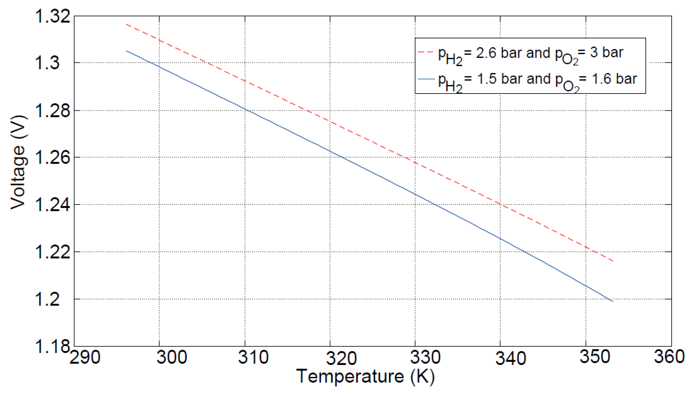
Figure 4 shows the thermodynamic potential of two different pairs of reactant pressures as a function of the temperature. The potential rises with increasing pressure and drops with increasing temperature. Typical PEM fuel cell temperatures lie in a range between 330 and 355 K.

2.3.2. Ohmic Voltage Drop

The first step to calculate ohmic voltage drop is to estimate the almost constant ohmic resistance $R_{\mathrm{ohm}}$. At medium current densities, ohmic resistance dominates fuel cell voltage drop, which leads to a nearly linear voltage drop. Within this part of the polarization curve the ohmic resistance can be calculated with the slope of the curve as follows:

$$R_{\mathrm{ohm}}={\displaystyle \frac{\Delta V}{\Delta I}}$$

(9)

With this, $V_{\mathrm{ohm}}$ can be calculated using the following Equation (10):

$$V_{\mathrm{ohm}}=R_{\mathrm{ohm}}·I_{\mathrm{FC}}$$

(10)

2.3.3. Nonlinear Voltage Drop

In the following, the derivation of activation and concentration resistances is presented. Afterward, the calculation of the nonlinear voltage drop across the capacitor is shown.

Activation rresistance

The activation resistance $R_{\mathrm{act}}$ can be calculated with I and $V_{\mathrm{act}}$ using the Tafel Equation.

$$V_{\mathrm{act}}=-{\displaystyle \frac{RT}{\alpha nF}}·ln\left(i_0\right)+{\displaystyle \frac{RT}{\alpha nF}}·ln\left(I\right)$$

(11)

Generalizing the term with the coefficients a and b where

$$a=-{\displaystyle \frac{RT}{\alpha nF}}·ln\left(i_0\right),b=-{\displaystyle \frac{RT}{\alpha nF}}$$

(12)

gives

$$V_{\mathrm{act}}=a-b·ln\left(I\right)$$

(13)

The resistance $R_{\mathrm{act}}$ can be calculated as follows.

$$R_{\mathrm{act}}={\displaystyle \frac{a-b·ln\left(I\right)}{I}}$$

(14)

According to [26], this can be simplified to:

$$R_{\mathrm{act}}=-b·\frac{ln\left(I\right)}{I}.$$

(15)

Concentration resistance

The concentration resistance $R_{\mathrm{conc}}$ can be calculated as follows.

$$R_{\mathrm{conc}}={\displaystyle \frac{V_{\mathrm{conc}}}{I}}={\displaystyle \frac{RT}{nFI}}·ln\left({\displaystyle \frac{-I}{I_{\max }}}\right)$$

(16)

The resistances $R_{\mathrm{conc}}$ and $R_{\mathrm{act}}$ can be calculated with the help of the Faraday constant F, the universal gas constant R, the temperature T, the number of electrons n as well as the current I and the maximum current $I_{\max }$.

Nonlinear rvoltage drop

Nonlinear voltage drop across activation and concentration resistance can be calculated with:

$${\displaystyle \frac{\mathrm{d}{v}_{\mathrm{d}}}{\mathrm{d}t}}={\displaystyle \frac{i}{C}}-{\displaystyle \frac{v_{\mathrm{d}}}{\tau }}$$

(17)

where $v_d$ is the voltage drop across $R_{\mathrm{act}}+R_{\mathrm{conc}}$. Calculation of the time constant $\tau$ depends on whether a positive or negative current step is occuring. In the event of a negative current step ($i_{\mathrm{t}2}<i_{\mathrm{t}1}$), $\tau$ can be determined with Equation (18):

$${\tau }_{\mathrm{negStep}}=C_{\mathrm{dl}}·(R_{\mathrm{act}}+R_{\mathrm{conc}})={\displaystyle \frac{C_{\mathrm{dl}}·(V_{\mathrm{act}}+V_{\mathrm{conc}})}{i_{\mathrm{FC}}-i_C}}$$

(18)

where $i_{\mathrm{FC}}$ is the fuel cell current, and $i_C$ is the capacitor current.

In case of a positive current step ($i_{\mathrm{t}2}>i_{\mathrm{t}1}$) $\tau$ has to be calculated with Equation (19):

$${\tau }_{\mathrm{posStep}}=C_{\mathrm{dl}}·R_{\mathrm{ohm}}={\displaystyle \frac{C_{\mathrm{dl}}·V_{\mathrm{ohm}}}{i_{\mathrm{FC}}}}$$

(19)

2.3.4. Simulation Results of the Double Layer Effect

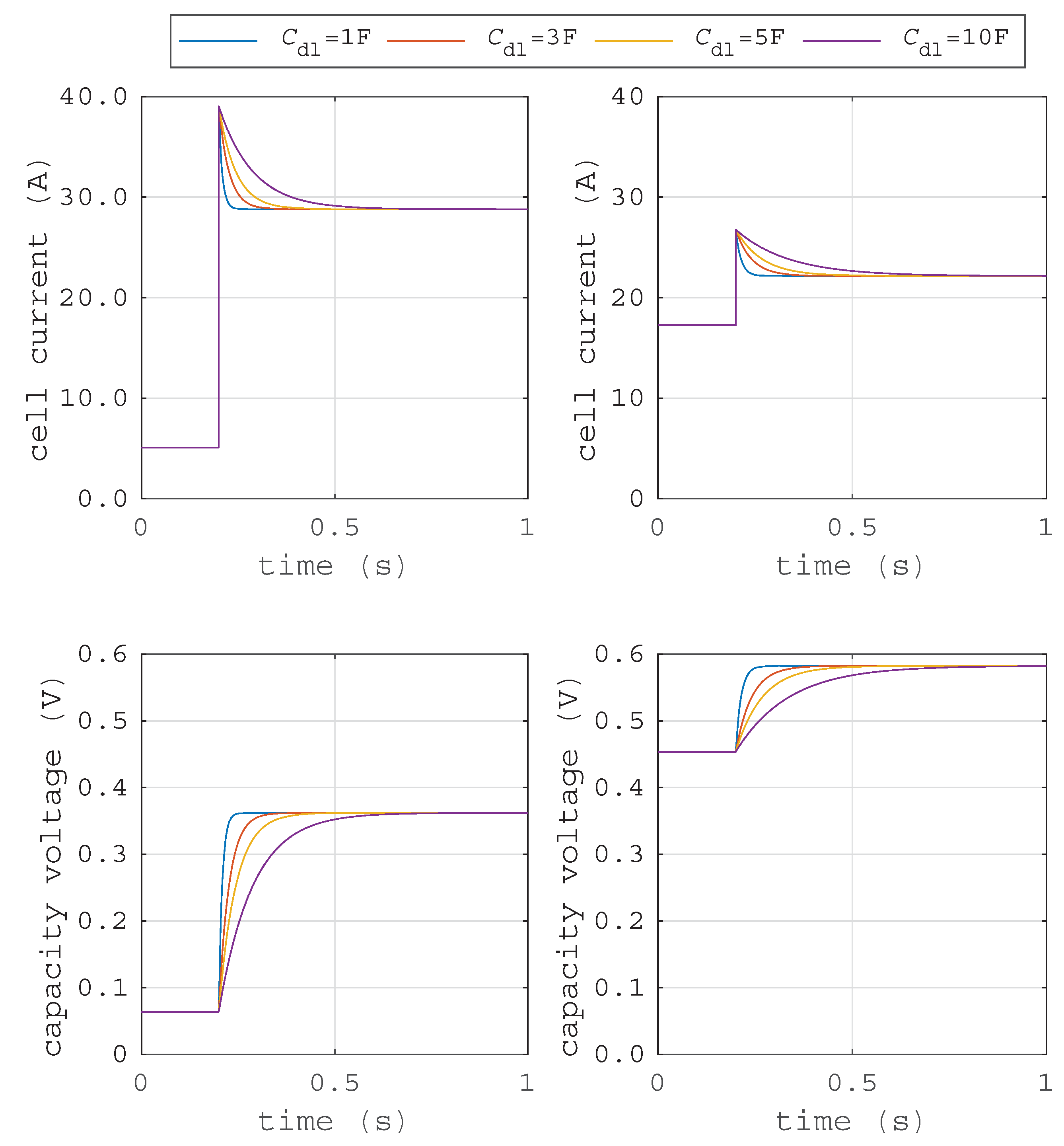
Different values for the double layer capacity can be found in the literature. In Figure 5, the simulation results of the double layer capacity, based on the representative electrical circuit (cf. Figure 3), during a short circuit are shown. The different curves show the current and voltage flows over time caused by the double layer effect for different capacities. For demonstration, a short circuit of a fuel cell system at two different operating points (partial load and maximum power point) are simulated with the Simscape package of Matlab/Simulink.

Table 1. Simulation parameters. $R_{\mathrm{act}}$ and $R_{\mathrm{conc}}$ are calculated by the described equations.

Operation	I	${\mathit{R}}_{\mathsf{load}}$	${\mathit{T}}_{\mathsf{OP}}$	${\mathit{E}}_{\mathsf{nernst}}$	${\mathit{I}}_{\mathsf{lim}}$	n	$\mathit{\alpha }$	${\mathit{R}}_{\mathsf{ohm}}$	${\mathit{R}}_{\mathsf{act}}$	${\mathit{R}}_{\mathsf{conc}}$
partial load	$4.8$$\mathrm{A}$	$0.2$$\mathsf{\Omega }$	$353.15$$\mathrm{K}$	$1.2$$\mathrm{V}$	20$\mathrm{A}$	2	0.5	$0.0233$$\mathsf{\Omega }$	$0.01$$\mathsf{\Omega }$	$0.0042$$\mathsf{\Omega }$
maximum power	$11.8$$\mathrm{A}$	$0.05$$\mathsf{\Omega }$	$353.15$$\mathrm{K}$	$1.2$$\mathrm{V}$	20$\mathrm{A}$	2	0.5	$0.0233$$\mathsf{\Omega }$	$0.0065$$\mathsf{\Omega }$	$0.0130$$\mathsf{\Omega }$

lists the simulation parameters.

The capacity voltage $v_{\mathrm{d}}$ rises immediately, which requires a charge balancing of the double layer capacity. Therefore, a current flow through the short-circuit path occurs.

$$i_{C_{\mathrm{dl}}}=C_{\mathrm{dl}}\frac{\mathrm{d}{v}_{\mathrm{d}}}{\mathrm{d}t}$$

(20)

Higher capacity values lead to longer current flow times but not higher currents for the same operating point. Furthermore, the impact of the electrochemical double layer depends on the operating point of the fuel cell system. The capacitance of the electrochemical double layer is at its maximum at the cell’s open circuit voltage. A current drawn from the fuel cell leads to a decrease of the effective capacitance. Thus, the capacitance further decreases with increasing fuel cell current. If a short circuit occurs during partial load operation, the additional current flow due to a temporary charge balancing of the double layer capacity is higher when the current prior to short circuit is lower. Therefore, the additional capacitance current is at its maximum at the cell’s open circuit voltage, when zero net current is drawn from the fuel cell. After charge balancing during the short circuit, the double layer is rebuilding itself and a stationary short circuit current results.

Additionally, the duration of the current flow is very short, depending on the double layer capacity and the resistance ratio. The result of the investigated electrochemical double layer has shown that the fuel cell output current is increased by the amount of the transient double layer current. Finally, it can be shown that the electrochemical double layer has a positive impact on the short circuit capability of a fuel cell system. Therefore, tripping of a conventional overcurrent protection might be possible. Yet, once again, the additional current depends on the operating point prior to the fault event, and the tripping is not guaranteed for every fault/load situation.

2.4. The Gas Diffusion Effect

The next investigated transient effect is gas diffusion. The calculation of the gas diffusion behavior is highly dynamic and very complex. Several simultaneous factors must be considered (e.g., gas pressure, temperature, diffusion constants of the reactants, material of the gas diffusion layer, the volume of the gas channel, pure oxygen or air supply). In summary, a general calculation of additional current during short circuit due to the gas diffusion phenomenon is not possible. That is why the following paragraphs describe the calculation by best case scenario—in case of a short circuit, the available oxygen in the gas channel is consumed immediately by the chemical reaction. With the oxygen partial pressure $p_{{\mathrm{O}}_2}$, the specific gas constant $R_{{\mathrm{O}}_2}$, the temperature T and the gas volume $V_{{\mathrm{O}}_2}$, the available oxygen mass $m_{{\mathrm{O}}_2}$ can be calculated with the ideal gas equation as follows:

$$m_{{\mathrm{O}}_2}={\displaystyle \frac{p_{{\mathrm{O}}_2}·V_{{\mathrm{O}}_2}}{R_{{\mathrm{O}}_2}·T}}$$

(21)

Assuming that oxygen reacts completely, the time dependence can be calculated. Multiplication with the current I on both sides leads to the following Equation (22):

$$t·I={\displaystyle \frac{m_{{\mathrm{O}}_2}·I}{{\dot{m}}_{{\mathrm{O}}_2}}}={\displaystyle \frac{m_{{\mathrm{O}}_2}}{\frac{{\dot{m}}_{{\mathrm{O}}_2}}{I}}}$$

(22)

The equation of the PEM fuel cell system for the oxygen reaction with the oxygen molar mass $M_{{\mathrm{O}}_2}$, the oxygen mass flow ${\dot{m}}_{{\mathrm{O}}_2}$ and the Faraday constant F is described as follows:

$${\displaystyle \frac{d{N}_{{\mathrm{O}}_2}}{dt}}={\displaystyle \frac{I}{4·F}}={\displaystyle \frac{{\dot{m}}_{{\mathrm{O}}_2}}{M_{\mathrm{O}2}}}$$

(23)

By conversion of Equation (23), using Equation (22) and the relationship $Q=I·t$, the stored electrical charge Q can be calculated as follows:

$$Q=I·t={\displaystyle \frac{m_{{\mathrm{O}}_2}}{\frac{M_{{\mathrm{O}}_2}}{4·F}}}$$

(24)

Based on the law of mass actions and the relationship $\tau =R·C$, it can be assumed that the current flow decreases exponentially, as described below.

$$I\left(t\right)=Q{\displaystyle \frac{\mathrm{d}{\mathrm{e}}^{\frac{-t}{\tau }}}{\mathrm{d}t}}$$

(25)

As previously described, this additional current depends on several constraints. Hence, it should not be considered to calculate the protection unit’s parameters.

3. Experiment

For further understanding of the described and simulated effect of the fuel cell system in Section 2, the general short circuit current capability of fuel cells is analyzed. To determine the magnitude of the fuel cell short circuit current, an experiment was carried out. In the following section, the experimental setup and the results of the external short circuit testing are presented.

3.1. Setup of Experiment

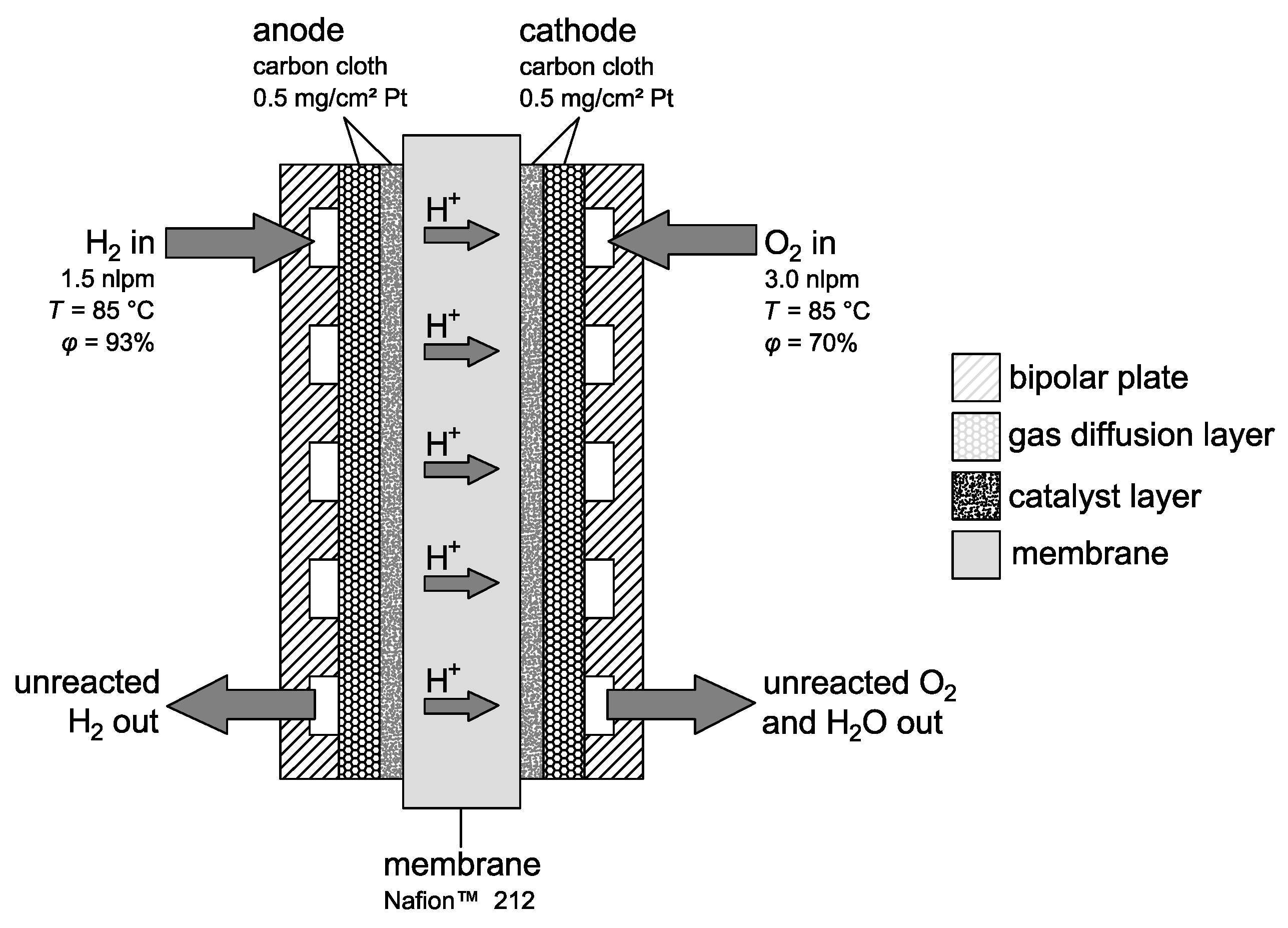
For the experiments, a single fuel cell with an active area of 25 $\mathrm{c}$$\mathrm{m}$${}^2$, as depicted in Figure 6, was built. The membrane was a Nafion^TM 212, and for the anode and cathode, a carbon cloth electrode with a catalyst loading of $0.5$ $\mathrm{m}$$\mathrm{g}$/$\mathrm{c}$$\mathrm{m}$${}^2$ Pt was used.

The membrane electrode assembly was manufactured by hot pressing the sandwich of electrode–membrane–electrode at 130 ${}^{\circ }\mathrm{C}$ under a pressure of 400 $\mathrm{N}$/$\mathrm{c}$$\mathrm{m}$${}^2$ for 3 $\min$. The fuel cell housing was balticFuelCells’ water cooled 25 $\mathrm{c}$$\mathrm{m}$${}^2$ quickCONNECTfixture, which allows for reproducible test procedures. The operating conditions of the gases were controlled by Greenlight Innovation’s G100 teststand, which could control the following parameters: gas and cell temperatures, gas humidity, pressure and mass flow rates. Cell temperature was kept constant at 80 ${}^{\circ }\mathrm{C}$ while anode and cathode gas temperatures were set to 85 ${}^{\circ }\mathrm{C}$. Anode and cathode humidity was set to 93% and 70%, respectively. Both anode and cathode supply were operated at ambient pressure. For mass flow, a constant flow rate was used. Hydrogen was fed with 1.5 nlpm (normal liters per minute), and air was fed with 3 nlpm. These high flow rates are a few times higher than typical stoichiometric ratios and were chosen to ensure:

• Stable gas temperatures because of large pipelines due to the used teststand,
• Proper supply of the cell with reactants during the short circuit tests; there is no risk of gas deficiency with this mass flow while testing the external short circuit of the cell.

Figure 7 shows the general experimental setup. The fuel cell is operated at several operating points with different external electrical resistances $R_{\mathrm{load}}$. A relay is installed parallel to the electrical load. The relay is controlled by a microcontroller, which changes the state of the MOSFET $S_{\mathrm{B}}$. When the relay closes the parallel circuit, the fuel cell current $i_{\mathrm{FC}}$ is almost shorted. Only a residual current $i_{\mathrm{load}}$ is flowing through $R_{\mathrm{load}}$, depending on the relay’s contact resistance.

Table 2. Parts of the test setup.

Part	Label	Manufacturer	Device	Relevant Device Parameters
load	$R_{\mathrm{load}}$	CGS—TE CONNECTIVITY	HSC200R10F	resistance: $0.1$$\mathsf{\Omega }$
				tolerance: 1%
relay	relay	Omron	G9EA-CA	current capacity: 100 $\mathrm{A}$
				contact resistance: $0.3$ $\mathrm{m}$$\mathsf{\Omega }$
oscilloscope		Teledyne Lecroy	MDA800A	sample rate: 10 $\mathrm{G}$$\mathrm{S}$ ${\mathrm{s}}^{-1}$
				A/D resolution: 12
voltage probe	$v_{\mathrm{FC}}$	Teledyne Lecroy	ZD1000	voltage range: 8 $\mathrm{V}$
				bandwidth: 1 $\mathrm{G}$$\mathrm{Hz}$
current probe load	$i_{\mathrm{load}}$	Teledyne Lecroy	CP 150 A	current range: 150 $\mathrm{A}$
				bandwidth: 10 $\mathrm{M}$$\mathrm{Hz}$
current probe	$i_{\mathrm{sc}}$	Teledyne Lecroy	AP015	current range: 30 $\mathrm{A}$
relay contacts				bandwidth: 50 $\mathrm{M}$$\mathrm{Hz}$

gives an overview of the relevant parts of the test-setup, the measurement and the test equipment for the values named in Figure 7. In order to approximate the stationary short circuit current, and thus be able to choose the correct operational points ($V_{\mathrm{OPn}},I_{\mathrm{OPn}}$), the fuel cell’s polarization and performance curves were recorded. After reaching a stable operating point, the fuel cell was short circuited for approximately $0.8$ s to minimize water production at the cathode and to keep the stress of the fuel cell tolerable. While the polarization curve was measured using an electronic load, the short circuit tests were conducted using a low inductive wire wound resistor configuration. Three different resistor configurations were applied:

• $R_{\mathrm{load}}=0.2\mathsf{\Omega }=\left(0.1\mathsf{\Omega }\right)+\left(0.1\mathsf{\Omega }\right)$,
• $R_{\mathrm{load}}=0.1\mathsf{\Omega }$,
• $R_{\mathrm{load}}=0.05\mathsf{\Omega }=\left(0.1\mathsf{\Omega }\right)\left|\right|\left(0.1\mathsf{\Omega }\right)$.

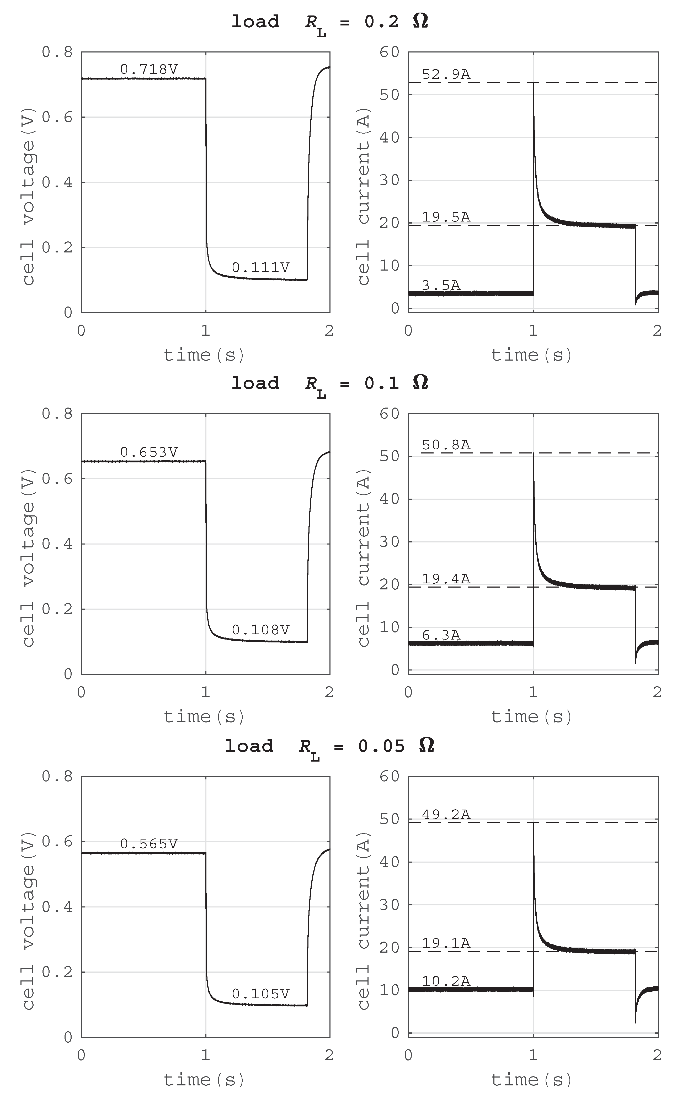
3.2. Results

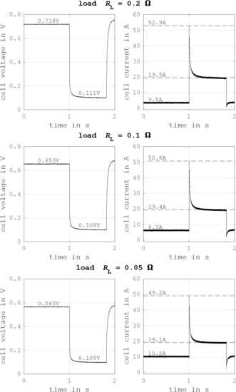
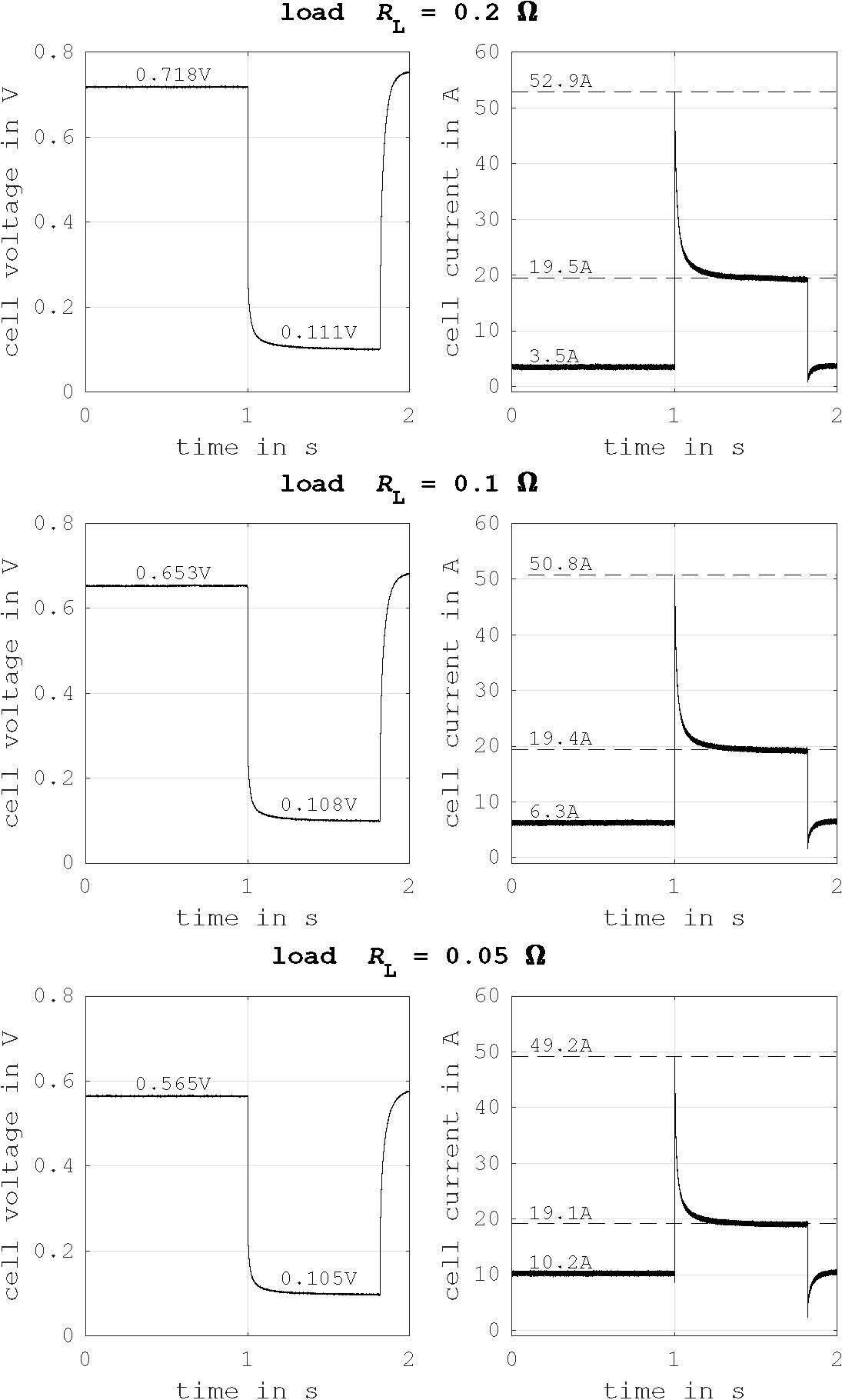
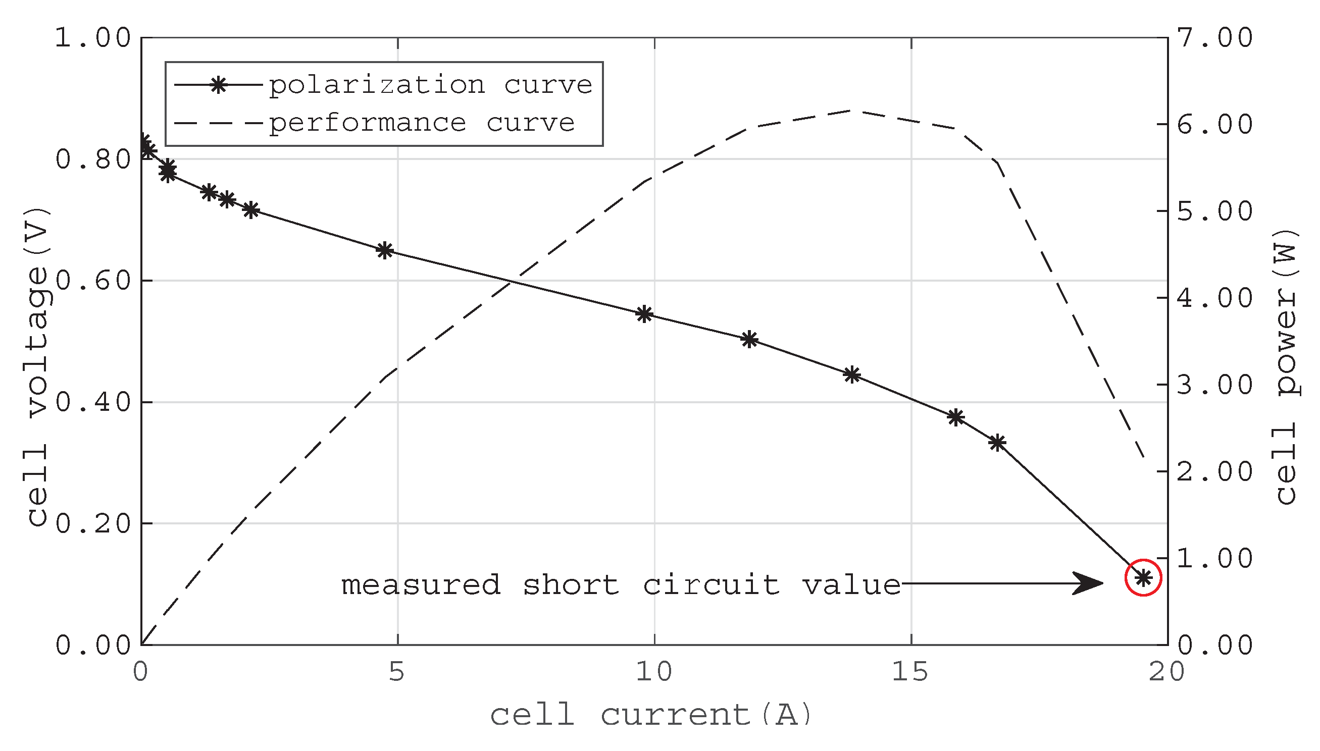
Figure 8 shows polarization and performance curves of the tested single cell, complemented by one data point from the measured stationary short circuit current, see Figure 9. According to [29], the stationary short circuit current $I_{\mathrm{sc}}$ to expect is two times the current at the nominal operating point $I_{\mathrm{nFC}}$ (Equation (26)).

$$I_{\mathrm{sc}}\approx 2·I_{\mathrm{nFC}}$$

(26)

The nominal operating current is typically given at a cell voltage of 0.5 $\mathrm{V}$ to 0.55 $\mathrm{V}$. Hence, the stationary short circuit current ranges from 19.6 $\mathrm{A}$ to 23.7 $\mathrm{A}$. As can be seen in Figure 9, the measured stationary current during the short circuit $I_{\mathrm{m}\mathrm{sc}}$ is on average $19.3$ $\mathrm{A}$. To estimate the available stationary short circuit current in case of $V_{\mathrm{FC}}=0$, Equation (27), resembling the Tafel Equation, is fitted to the data with the Matlab Curve Fitting Toolbox™. The calculated coefficients are: $a_{\mathrm{fit}}=0.1671\mathrm{V}$, $b_{\mathrm{fit}}=22\mathrm{A}$, $c_{\mathrm{fit}}=0.2167\mathrm{A}$, and $d_{\mathrm{fit}}=0.01038\mathsf{\Omega }$.

$$V_{\mathrm{FC}}\left(I_{\mathrm{FC}}\right)=a_{\mathrm{fit}}·log\frac{b_{\mathrm{fit}}-I_{\mathrm{FC}}}{c_{\mathrm{fit}}}-d_{\mathrm{fit}}·I_{\mathrm{FC}}$$

(27)

Then, Taylor’s theorem of the first order at $I_{\mathrm{m}\mathrm{sc}}=19.3\mathrm{A}$ is calculated for Equation (27) and solved for $I_{\mathrm{FC}}(V_{\mathrm{FC}}=0)$ (see Equation (28)). This theoretical value cannot be reached because it is physically impossible to create a short circuit with zero resistance. Yet, the calculated value confirms the results of [29].

$$\begin{array}{cc}\hfill I_{\mathrm{FC}}(V_{\mathrm{FC}}=0)& =I_{\mathrm{m}\mathrm{sc}}+\frac{V_{\mathrm{FC}}\left(I_{\mathrm{m}\mathrm{sc}}\right)}{\frac{a_{\mathrm{fit}}}{b_{\mathrm{fit}}-I_{\mathrm{m}\mathrm{sc}}}+d_{\mathrm{fit}}}\hfill \\ \hfill & =20.8132\mathrm{A}\hfill \end{array}$$

(28)

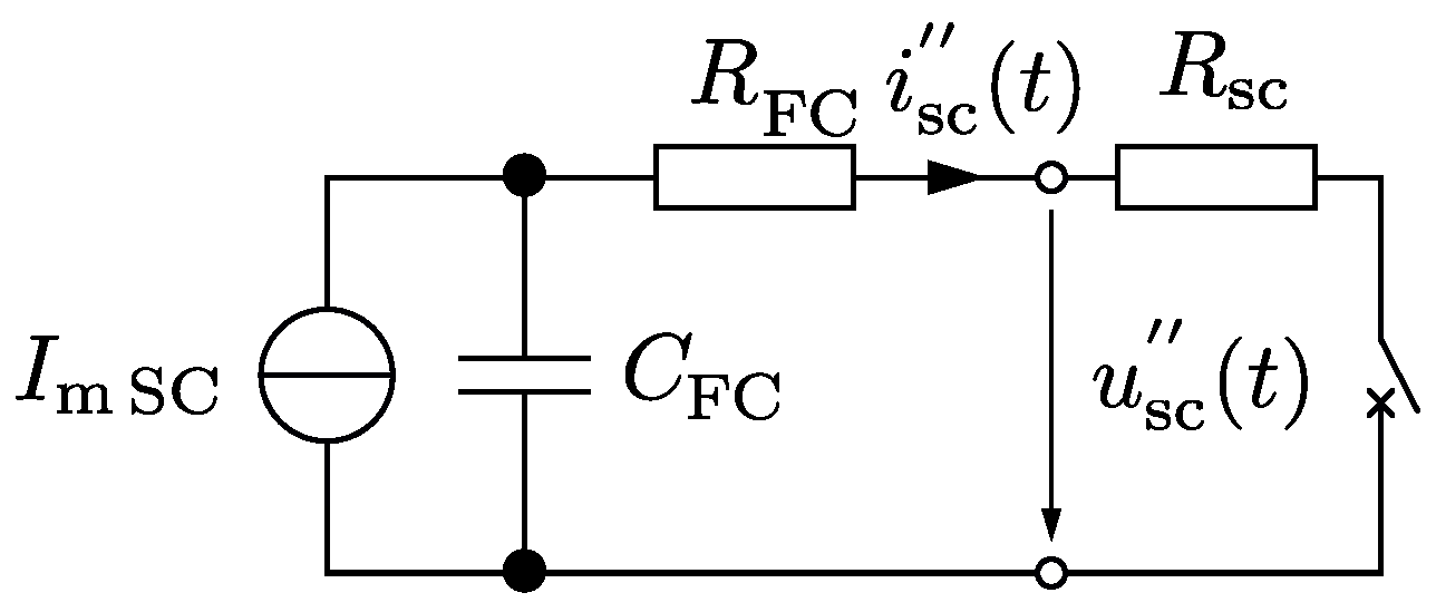
Figure 9 shows the short circuit curves for three different operating points. From the top to the bottom, the operating point is nearing the maximum power point. The results show clearly how the transient short circuit current is lower for operating points near the maximum power point. Furthermore, the stationary short circuit current seems independent of the operating point right before the experiment. The measurements of Figure 9 confirm that the transient short circuit current $i_{\mathrm{sc}}^{″}\left(t\right)$ is driven by a cell capacity $C_{\mathrm{FC}}$: it can be described by the equivalent circuit of Figure 10. Thus, $i_{\mathrm{sc}}^{″}\left(t\right)$ can be calculated with Equation (29), where the resistance R is the sum of the internal resistance of the fuel cell $R_{\mathrm{FC}}$ and the fault resistance $R_{\mathrm{sc}}$.

$$i_{\mathrm{sc}}^{″}\left(t\right)=\frac{V_{\mathrm{FC}}(t=0)}{R}exp\left(-\frac{t}{R{C}_{\mathrm{FC}}}\right)+I_{\mathrm{m}\mathrm{sc}}\left(1-exp\left(-\frac{t}{R{C}_{\mathrm{FC}}}\right)\right)$$

(29)

Table 3. Calculated values for double layer capacity and short circuit resistance.

Load	${\mathit{R}}_{\mathsf{load}}$	$\mathsf{\Omega }$	0.2	0.1	0.05
resistance	R	$\mathsf{\Omega }$	0.0146	0.0140	0.0127
cell capacity	$C_{\mathrm{FC}}$	$\mathrm{F}$	1.6634	1.5273	1.2260
cell capacity per cell area	$\frac{C_{\mathrm{FC}}}{A}$	$\mathrm{F}/\mathrm{c}{\mathrm{m}}^2$	0.0665	0.0611	0.0490

shows calculated values for the effective cell capacities and the resistances of the short circuit path for the three tested loads. The resulting cell capacity of a fuel cell stack is reduced because several cell capacities are connected in series. Hence, expected energy of the transient current is smaller than in the experiments.

3.3. Implications Regarding Evaluation of Grid Protection

An essential part of grid planning is the evaluation of possible fault conditions. Therefore, calculations of over currents and short circuit currents are done in various configurations of the considered system to determine trigger parameters of protection units as well as needed mechanical strength of installation components.

As can be seen in the time–current curves of Figure 5, the simplified equivalent circuit diagram of Figure 3 estimates different stationary short circuit currents for different load conditions prior to fault. The experimental results show a different behavior: similar constant stationary short circuit currents. An improved model with dynamic, nonlinear resistances $R_{\mathrm{act}}$ and $R_{\mathrm{conc}}$ would result in two current feedback control loops, see Equations (14) and (16). Such loops increase calculation afford of short circuit calculations of complex system configurations. Hence, it is not a favorable option for the evaluation of protection systems.

The simple model of Figure 10 is only valid for bolted faults ($R_{\mathrm{sc}}\approx 0$); in the case of faults with impedances, it would overestimate the fault current. This overestimation leads to false trigger parameters of protection devices. Thus, grid protection as well as proper selectivity of the protection elements is not ensured. Hence, a model comprising simple and well known circuit elements is needed to evaluate the protection systems for fault conditions like over load currents, faults with impedances and bolted faults.

4. Alternative Fuel Cell Model for Estimation of Short Circuit Behavior

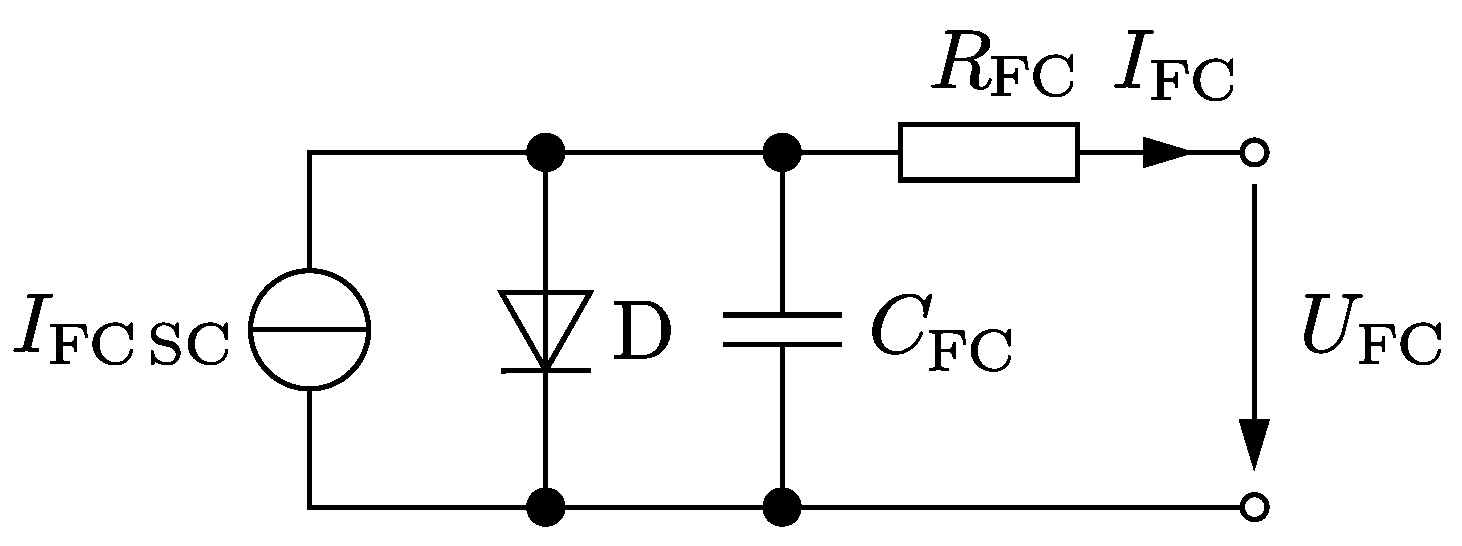
In this chapter, a new modeling approach of the short circuit behavior of fuel cells with simple lumped circuit elements is presented. It can be used in circuit simulation programs to determine the fuel cell system’s fault currents due to over load situations, faults with impedances ($R_{\mathrm{sc}}\approx 50\mathrm{m}\mathsf{\Omega }to500\mathrm{m}\mathsf{\Omega }$ for systems with a nominal voltage of above 100 volt) and bolted faults. This approach is based on the similarities of fuel cell characteristics to photovoltaic cells. The benefit of the similarities is that the protection schemes of photovoltaic installations that are well known and internationally standardized can be easily compared and adapted to fuel cell systems. Subsequently, the model is validated using our data.

4.1. Novel Modeling Approach

Typically, the stationary behavior of a photovoltaic cell is described by the equivalent circuit that comprises a current source depending on the insolation parallel to a diode and a series resistor. The mathematical formulation of this circuit results in Equation (30). This formula resembles Equation (27). Furthermore, the polarization curve of Figure 8 is also comparable with photovoltaic current to voltage curves if the activation losses of fuel cells at low currents are neglected. Especially in over current and short-circuit current considerations, this assumption is valid.

$$V_{\mathrm{PV}}\left(I_{\mathrm{PV}}\right)=log\left(\frac{I_{\mathrm{ph}}-I_0-I_{\mathrm{PV}}}{I_0}\right)-R_{\mathrm{PV}}{I}_{\mathrm{PV}}$$

(30)

Hence, an alternative equivalent circuit for a fuel cell can be obtained by a combination of the equivalent circuit of a photovoltaic cell, c.f. [30], with the circuit of Figure 10. This results in the alternative model of Figure 11.

4.2. Model Validation

The modeling approach of Figure 11 is implemented in Matlab/Simulink using the Simscape addition. For the diode, an exponential model is used. Matlab/Simscape offers the possibility to calculate the diode’s parameter $I_{\mathrm{s}}$ and N by two values of the diode voltage $V_{\mathrm{D}}$ and current $I_{\mathrm{D}}$ from the I-V-curve. Hence, the diode part of Equation (27) is solved for $I_{\mathrm{FC}}$. Since the diode current is $I_{\mathrm{D}}=b_{\mathrm{fit}}-I_{\mathrm{FC}}$, Equation (31) can be used to calculate the needed values. For the values of $a_{\mathrm{fit}}$ and $c_{\mathrm{fit}}$, see Section 3.2.

$$I_{\mathrm{D}}\left(V_{\mathrm{D}}\right)=c_{\mathrm{fit}}{\mathrm{e}}^{\frac{V_{\mathrm{D}}}{a_{\mathrm{fit}}}}$$

(31)

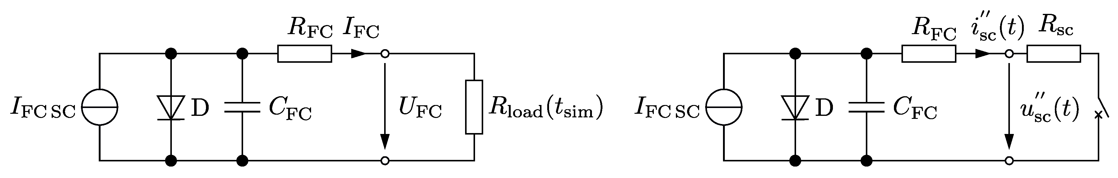
Two simulations are performed with the model: the polarization curve is simulated using different loads and a transient simulation is carried out for a load of $R_{\mathrm{load}}=0.05\mathsf{\Omega }$. Both configurations are shown in Figure 12.

Equation (32) represents the load for a simulation time of $t_{\mathrm{sim}}$ = 100 $\mathrm{s}$.

$$R_{\mathrm{load}}\left(t_{\mathrm{sim}}\right)=1\mathsf{\Omega }-\frac{1\mathsf{\Omega }}{100\mathrm{s}}·t_{\mathrm{sim}}$$

(32)

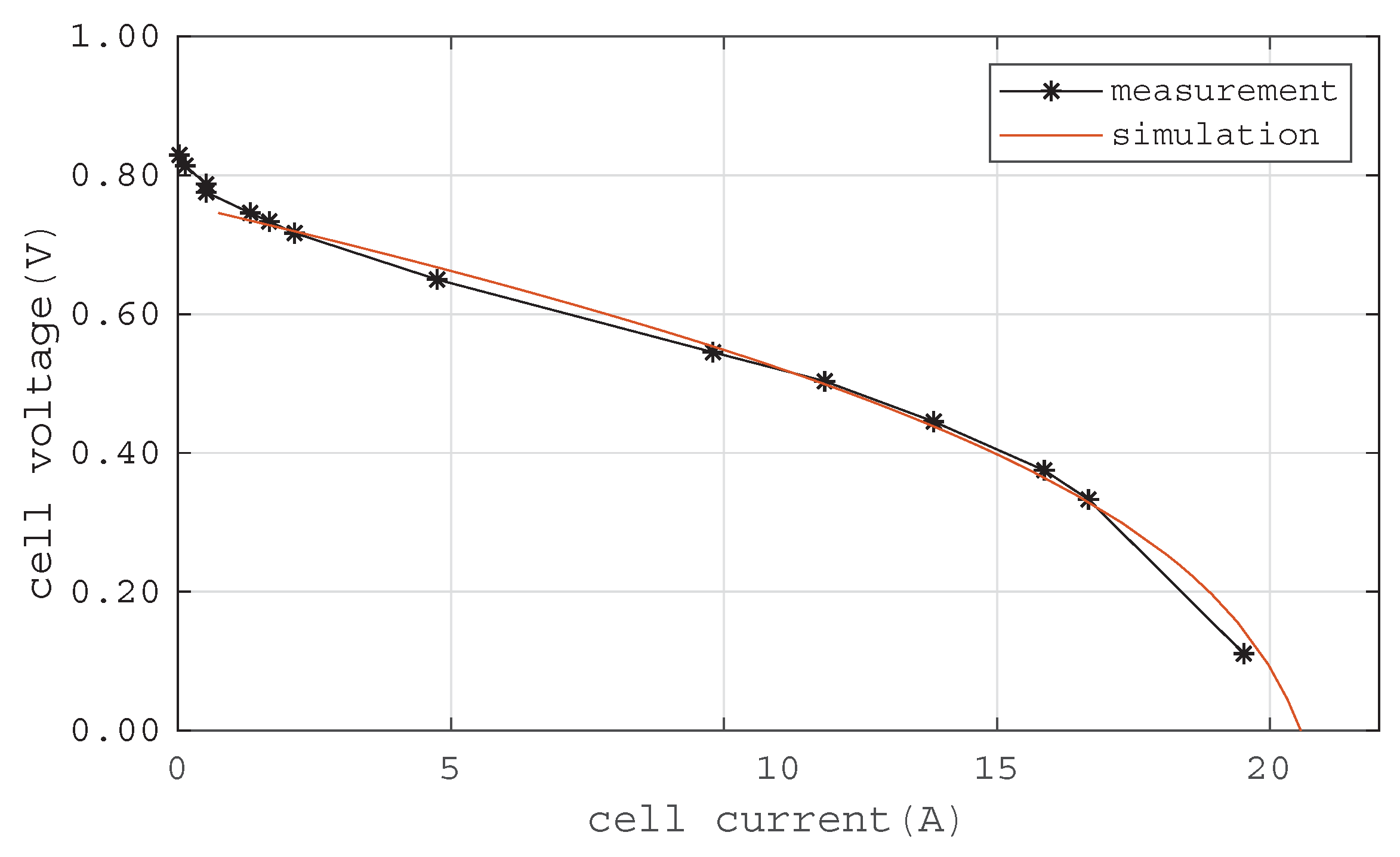
The value d from Section 3.2 is the value for the internal resistance $R_{\mathrm{fc}}$ of Figure 11. $I_{\mathrm{FC}\mathrm{SC}}$ equals the fuel cell current at zero voltage that was calculated by Equation (28) in Section 3.2. The double layer capacity has a value of $1.6$ $\mathrm{F}$ (cf. Table 3). As can be seen in Figure 13, the deviation between measurement and simulation is small for the stationary behavior of the fuel cell.

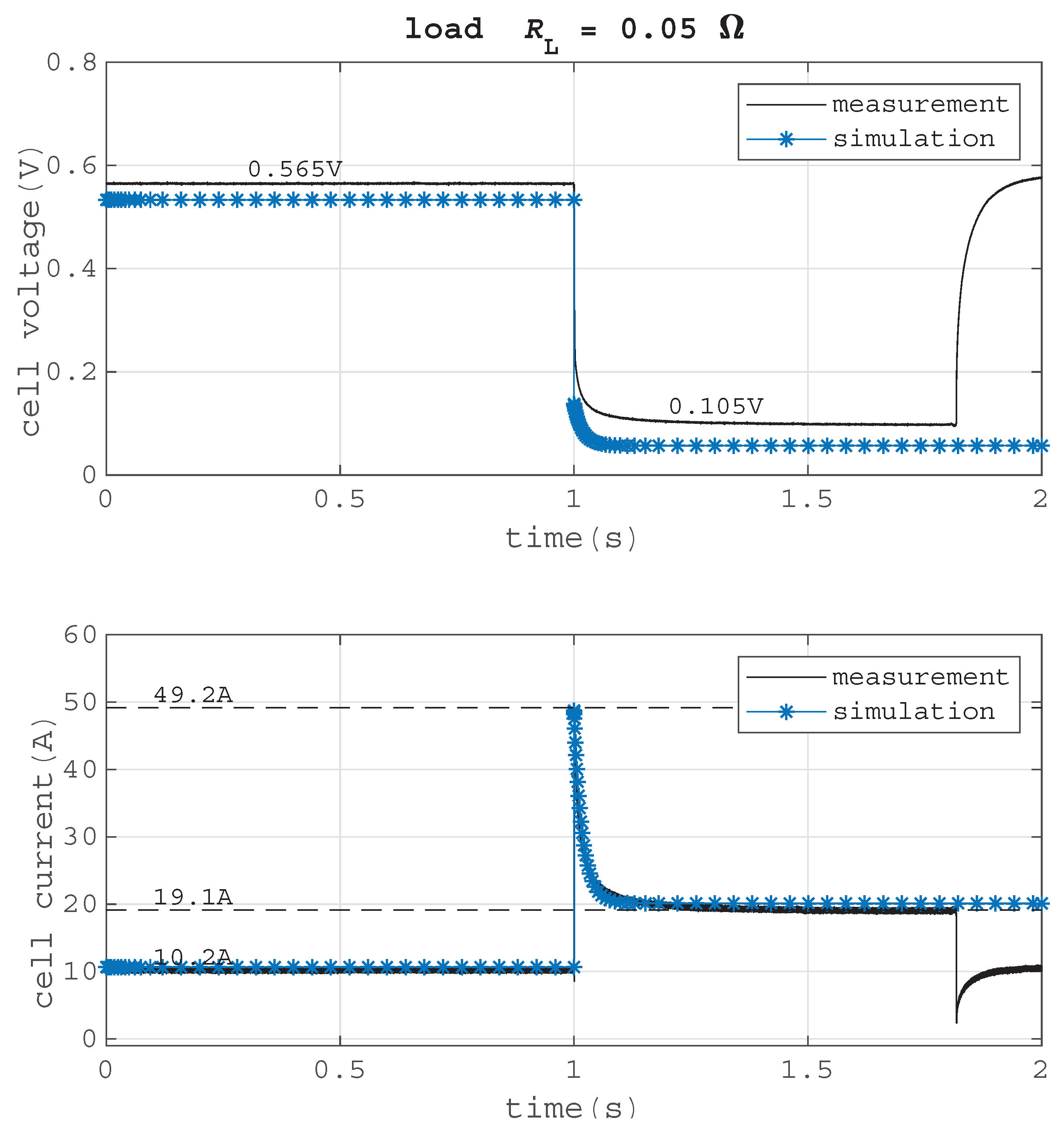
In Figure 14, the transient behavior of a short circuit at a load of $R_{\mathrm{load}}=$ 0.05 $$ is compared with the simulation model. The short circuit resistance is $R_{\mathrm{sc}}=5\mathrm{m}\mathsf{\Omega }$. A negative offset in the cell voltage curve of the simulation can be seen. This difference occurs because the connection resistance between fuel cell and load is not taken into account in the simulation model. Yet, the short circuit current profile, which was the aim of this model, is accurate.

5. Conclusions

The aim of the investigations was to analyze and understand the short circuit current behavior of fuel cells to derive a method to validate protection systems for fuel cell systems. Therefore, the two main transient effects that describe the short circuit capability of a fuel cell system were investigated in detail. Furthermore, external short circuit tests on a single PEM fuel cell validated the simulation results based on the mathematical description. Here, the pumping power of fuel cells, which is an important factor for the fuel cell net power, is not considered but should be examined in future work [31].

It could be shown that fuel cell systems have a reduced short circuit capability and stationary short circuit currents are in the range of 200% of the nominal current regardless of the operating point before the shorting. Only the transient current depends on the operating point due to the charge balancing of the double layer and amounts to at least two to three times the stationary short circuit current. A higher load resistance (small fuel cell current) prior to a short circuit event causes a higher charge balancing of the double layer capacity during the transition from operating point to the stationary short circuit current. Hence, a higher transient short circuit current occurs.

The result of the theoretical analysis, simulations and experimental tests is an equivalent circuit diagram that is valid for over load, impedance fault and bolted fault situations of fuel cell systems. Model validation shows very good agreement between the simulation results and our experimental data. As a result, the short circuit capability of a PEM fuel cell system can easily be estimated and used to develop new grid protection systems for this type of limited short circuit generation unit. The developed equivalent circuit diagram is similar to the equivalent circuit diagram of photovoltaic systems. Hence, the protection methods and solutions of photovoltaic systems can be adapted to fuel cell systems.

As a consequence of the limited short circuit current, existing grid protection mechanisms have to be adapted [32,33,34] for single fuel cell systems. The analysis of additional short circuit current flow indicates that an overcurrent protection is not satisfactory. With the usage of electrically controllable fuel cells, higher short circuits could be possible [35]. The developed fuel cell model in this paper enables the simulation of the transient short circuit behavior.

References

- Marx, N.; Hissel, D.; Gustin, F.; Boulon, L.; Agbossou, K. On the sizing and energy management of an hybrid multistack fuel cell—Battery system for automotive. Int. J. Hydrog. Energy 2017, 42, 1518–1526. [Google Scholar]
- Liu, Y.; Lehnert, W.; Janßen, H.; Samsun, R.C.; Stolten, D. A review of high-temperature polymer electrolyte membrane fuel-cell (HT-PEMFC)-based auxiliary power units for diesel-powered road vehicles. J. Power Sources 2016, 311, 91–102. [Google Scholar] [CrossRef]
- Garche, J.; Jürissen, L. Applications of Fuel Cell Technology: Status and Perspectives. Electrochem. Soc. Interface 2015, 24, 39–43. [Google Scholar] [CrossRef]
- Daud, W.R.W.; Rosli, R.E.; Majlan, E.H.; Hamid, S.A.A.; Mohamed, R.; Husaini, T. PEM fuel cell system control: A review. Renew. Energy 2017, 113, 620–638. [Google Scholar] [CrossRef]
- Friedrich, K.A.; Kallo, J.; Schirmer, J.; Schmitthals, G.; Senturia, S. Fuel Cell Systems for Aircraft Application. ECS Trans. 2009, 25, 193–202. [Google Scholar]
- Grumm, F.; Schumann, M.; Meyer, M.F.; Lücken, A.; Schulz, D. Novel Protection System for Electrical Systems with Limited Short-Circuit Current. In Proceedings of the 2018 2nd European Conference on Electrical Engineering and Computer Science (EECS), Bern, Switzerland, 20–22 December 2018. [Google Scholar]
- Agbossou, K.; Kolhe, M.; Hamelin, J.; Bose, T.K. Performance of a stand-alone renewable energy system based on energy storage as hydrogen. IEEE Trans. Energy Convers. 2004, 19, 633–640. [Google Scholar] [CrossRef]
- Konara, K.M.S.Y.; Kolhe, M.L.; Nishimura, A. Grid integration of PEM fuel cell with multiphase switching for maximum power operation. In Proceedings of the 2016 IEEE International Conference on Power System Technology (POWERCON), Wollongong, NSW, Australia, 28 September–1 October 2016. [Google Scholar]
- Shamim, N.; Bilbao, A.; Reale, D.; Bayne, S. Analysis of Grid Connected Fuel Cell Power System Integrated with Supercapacitor. In Proceedings of the 2018 IEEE Green Technologies Conference (GreenTech), Austin, TX, USA, 4–6 April 2018. [Google Scholar]
- Han, S.; Sun, L.; Shen, J.; Pan, L.; Lee, K.Y. Optimal Load-Tracking Operation of Grid-Connected Solid Oxide Fuel Cells through Set Point Scheduling and Combined L1-MPC Control. Energies 2018, 11, 801. [Google Scholar] [CrossRef]
- Ramy, S.; Hatem, A.; Mami, A. Study and design of a power management system using two-stage controller for PEM fuel cell vehicles. In Proceedings of the 2016 7th International Renewable Energy Congress (IREC), Hammamet, Tunisia, 22–24 March 2016. [Google Scholar]
- Mi, C.; Masrur, M.A.; Gao, D.W. Hybrid Electric Vehicles: Principles and Applications with Practical Perspectives, 1st ed.; Wiley: Hoboken, NY, USA, 2011; pp. 3–8. [Google Scholar]
- Bernard, J.; Delprat, S.; Guerra, T.; Buchi, F. Fuel efficient power management strategy for fuel cell hybrid powertrains. Control Eng. Pract. 2010, 18, 408–417. [Google Scholar] [CrossRef]
- Keller, S.; Christmann, K.; Gonzalez, M.S.; Heuer, A. A Modular Fuel Cell Battery Hybrid Propulsion System for Powering Small Utility Vehicles. In Proceedings of the 2017 IEEE Vehicle Power and Propulsion Conference (VPPC), Belfort, France, 11–14 December 2017. [Google Scholar]
- Meng, X.; Li, Q.; Zhang, G.; Wang, T.; Chen, W.; Cao, T. A Dual-Mode Energy Management Strategy Considering Fuel Cell Degradation for Energy Consumption and Fuel Cell Efficiency Comprehensive Optimization of Hybrid Vehicle. IEEE Access 2019, 7, 134475–134487. [Google Scholar] [CrossRef]
- Moir, I.; Seabridge, A. Aircraft Systems. In Aircraft Systems, 3rd ed.; Wiley: Hoboken, NY, USA, 2011; pp. 227–229. [Google Scholar]
- Sarlioglu, B.; Morris, C.T. More Electric Aircraft: Review, Challenges, and Opportunities for Commercial Transport Aircraft. IEEE Trans. Transp. Electrif. 2015, 1, 54–64. [Google Scholar] [CrossRef]
- Mat, Z.B.A.; Kar, Y.B.; Saiful, H.B.A.H.; Talik, N.A.B. Proton Exchange Membrane (PEM) and Solid Oxide (SOFC) Fuel Cell Based Vehicles—A Review. In Proceedings of the ICITE 2017, Singapore, 1–3 September 2017. [Google Scholar]
- Heuck, K.; Dettmann, K.-D.; Schulz, D. Electrical System of Aircraft (In German: Bordnetz von Flugzeugen). In Electrical Energy Supply (Elektrische Energieversorgung); Heuck, K., Schulz, D., Eds.; Springer Vieweg: Wiesbaden, Germany, 2013; pp. 95–98. (In German) [Google Scholar]
- Bizon, N.; Oproescu, M.; Raceanu, M. Efficient energy control strategies for a Standalone Renewable/Fuel Cell Hybrid Power Source. Energy Convers. Manag. 2015, 90, 93–110. [Google Scholar] [CrossRef]
- Bhise, D.R.; Kankale, R.S.; Jadhao, S. Impact of Distributed Generation on Protection of Power System. In Proceedings of the ICIMIA 2017, Piscataway, India, 21–23 February 2017. [Google Scholar]
- Wu, S.; Li, Y. Fuel cell applications on more electrical aircraft. In Proceedings of the 17th International Conference on Electrical Machines and Systems (ICEMS), Hangzhou, China, 22–25 October 2014; pp. 198–201. [Google Scholar] [CrossRef]
- Eelman, S.; del Pozo y de Poza, I.; Krieg, T. Fuel Cell APU’s in Commercial Aircraft —An Assesment of SOFC And PEMFC Concepts, 2004. In Proceedings of the 24th Congress of International Council of the Aeronautical Sciences, Yokohama, Japan, 29 August–3 September 2004. [Google Scholar]
- Adzakpa, K.P.; Agbossou, K.; Dubé, Y.; Dostie, M.; Poulin, A. PEM Fuel Cells Modeling and Analysis through Current and Voltage Transient Behaviors. IEEE Trans. Energy Convers. 2008, 23, 581–591. [Google Scholar] [CrossRef]
- Schindele, L. Application of a Power Elecronic Actuator Parameter Identification and Optimal Management of PEM Fuel Cell Systems (Einsatz eines leistungselektronischen Stellglieds zur Parameteridentifikation und optimalen Betriebsführung von PEM Brennstoffzellensystemen). Ph.D. Thesis, Karlsruhe Institute of Technology, Karlsruhe, Germany, 27 March 2006. (In German). [Google Scholar]
- Wang, C.; Nehrir, H.; Shaw, S.R. Dynamic Models and Model Validation for PEM Fuel Cells Using Electrical Circuits. IEEE Trans. Energy Convers. 2005, 20, 442–451. [Google Scholar] [CrossRef]
- O’Hayre, R.; Cha, S.W.; Collela, W.; Prinz, F.B. Reversible Voltage Variation with Concentration: Nernst Equation. In Fuel Cell Fundamentals; John Wiley & Sons, Inc.: Hoboken, NJ, USA, 2016; pp. 50–54. [Google Scholar]
- Lazarou, S.; Pyrgioti, E.; Alexandridis, A.T. A simple electric model for proton exchange membrane fuel cells. J. Power Sources 2009, 190, 380–386. [Google Scholar] [CrossRef]
- Silva, R.E.; Harel, F.; Jemei, S.; Gouriveau, R.; Hissel, D.; Boulon, L.; Agbossou, K. Proton Exchange Membrane Fuel Cell Operation and Degradation in Short-Circuit. Fuel Cells 2014, 14, 894–905. [Google Scholar] [CrossRef]
- Mahmoud, Y.; El-Saadany, E.F. A Photovoltaic Model With Reduced Computational Time. IEEE Trans. Ind. Electron. 2015, 62, 3534–3544. [Google Scholar] [CrossRef]
- Zhang, X.; Higier, A.; Zhang, X.; Liu, H. Experimental Studies of Effect of Land Width in PEM Fuel Cells with Serpentine Flow Field and Carbon Cloth. Energies 2019, 12, 471. [Google Scholar] [CrossRef]
- Lücken, A.; Kut, T.; Dickmann, S.; Schulz, D. Fuel Cell System Optimization using Bypass Converters. IEEE Trans. Aerosp. Electron. Syst. 2014, 50, 170–179. [Google Scholar] [CrossRef]
- Lücken, A.; Lüdders, H.; Kut, T.; Dickmann, S.; Thielecke, F.; Schulz, D. Analysis of a new electrical converter architecture for fuel cell integration on overall system level (Analyse einer neuartigen elektrischen Konverterarchitektur zur Integration von Brennstoffzellen auf Gesamtsystemebene). In Proceedings of the 61. Deutscher Luft- und Raumfahrt Kongress, Berlin, Germany, 10–12 September 2012. (In German). [Google Scholar]
- Grumm, F.; Storjohann, J.; Lücken, A.; Meyer, M.F.; Schumann, M.; Schulz, D. Robust Primary Protection Device for Weight-Optimized PEM Fuel Cell Systems in High-Voltage DC Power Systems of Aircraft. IEEE Trans. Ind. Electron. 2019, 66, 5748–5758. [Google Scholar] [CrossRef]
- Schumann, M.; Grumm, F.; Friedrich, J.; Schulz, D. Electric Field Modifier Design and Implementation for Transient PEM Fuel Cell Control. WSEAS Trans. Circuits Syst. 2019, 18, 55–62. [Google Scholar]
Figure 1.
Characteristic polarization curve of a fuel cell.
Figure 2.
Time scales of the transient and dynamic phenomena in a Proton Exchange Membrane (PEM) fuel cell.
Figure 3.
Electrical equivalent circuit for the description of the effect of the electrochemical double layer on transient cell voltage and current.
Figure 4.
Thermodynamic potential as a function of temperature for two different pairs of reactant pressures.
Figure 5.
Time-current and time-voltage curves for different capacities: (left) at partial load operation; (right) at maximum power.
Figure 6.
Profile of a proton exchange membrane fuel cell with the employed materials.
Figure 7.
Setup of experiment for external short circuit tests.
Figure 8.
Measured polarization and performance curves of the tested fuel cell. The added value for the stationary short circuit current is marked by a red circle.
Figure 9.
Cell voltage and current behavior for an external short circuit for different ohmic loads: (top) Ohmic load of 0.2 , (middle) Ohmic load of 0.1 , (bottom) Ohmic load of 0.05 .
Figure 10.
Equivalent circuit diagram for the short circuit case of a fuel cell.
Figure 11.
Alternative model of a fuel cell for short circuit current estimation.
Figure 12.
Configurations of the two simulations to validate the model: (left) stationary simulation model for the polarization curve, (right) model for the transient behavior during a short circuit.
Figure 13.
Comparison of measured and simulated polarization curve.
Figure 14.
Comparison of measured and simulated fuel cell behavior at 0.05 : (top) transient voltage, (bottom) transient current.