Building a Better Baseline for Residential Demand Response Programs: Mitigating the Effects of Customer Heterogeneity and Random Variations

Abstract

Peak-time rebates offer an opportunity to introduce demand response in electricity markets. To implement peak-time rebates, utilities must accurately determine the consumption level if the program were not in effect. Reliable calculations of customer baseline load elude utilities and independent system operators, due to factors that include heterogeneous demands and random variations. Prevailing research is limited for residential markets, which are growing rapidly with the presence of load aggregators and the availability of smart grid systems. Our research pioneers a novel method that clusters customers according to the size and predictability of their demands, substantially improving existing customer baseline calculations and other clustering methods.

1. Introduction

Smart grid systems provide real-time capability for managing and monitoring electric usage. With smart grid technology, demand response (DR) offers a cost-effective alternative to increasing electricity supply, when dealing with a small number of capacity-constrained hours. For purposes of this article, DR refers to programs where customers are paid “to reduce their consumption relative to an administratively set baseline level of consumption.” [1]. While economists have long endorsed dynamic prices such as real-time pricing (RTP) that vary continuously to improve electric system efficiency, regulators have hesitated to implement these programs, particularly for residential customers. Borenstein [2] has noted that customers have resisted these rates, due to their complexity and the possibility of much higher bills from price surges. To gain greater customer participation, electricity load-serving entities (LSEs) have introduced DR offerings, such as peak-time rebate (PTR), that credit customers for reducing their use during event hours rather than charging a premium during high demand hours.

Some observers, such as in [3], suggest that subsidies and premiums are equivalent in their effects on load. At the margin, the cost to reducing load is the same whether there is a penalty or a subsidy. However, economists find evidence that customers respond differently to rewards than to penalties (for example, see Gneezy et al. [4]). There is also a difference in the mechanisms. Unlike RTP, programs such as PTR require providers to determine load reduction. The predominant method is to pay customers the difference between their actual usage and a calculated customer baseline load (CBL), a measure of energy customers would have consumed at their former rate.

The use of a CBL introduces considerable complications. First, the CBL is counterfactual, as the LSE cannot observe what the customer on DR would have used at the previous rate. To calculate a CBL, electricity providers have used several methods, typically based on historical data during non-event periods. However, actual event conditions are likely to differ from historical use during non-event periods, so the CBLs will be, at best, approximations of event-period use. Customer demands can differ during the two periods, due to such factors as weather conditions, different customer activities, and simply random shocks.

There are additional complications that, at the extreme, can result in the provider “paying for nothing,” and customers “free riding.” Williamson and Marrin [5] identify random variation as one circumstance where “free riding” and “paying for nothing” can arise. Consider two customers with equal average demands, but differing demand volatility. CBLs commonly pay the wholesale rate for reductions below baseline, but charge customers the retail rate for consumption above baseline. The customer with larger demand fluctuations will get a larger rebate, given that wholesale rates during event days generally exceed retail rates. In fact, the customer can get a rebate without changing behavior at all, getting paid PTR for use below the baseline, while paying the traditional retail rate for use above the baseline. Williamson and Marrin predicted revenue losses for two California utilities—Southern California Edison (SCE) and San Diego Gas and Electric (SDG&E)—with PTR programs, and found that for residential customers, one-third to two-thirds of payouts are due to random variations and not actual load reductions in response to price incentives. They note that regulated utilities can pass these costs on to customers, which reduces the utility’s incentive to analyze whether demand reductions are real or illusory. One impediment to CBL that has received extensive attention from the literature is customer behavior to game the system by inflating the baseline. We are unable to consider gaming, as the customers we study are not yet subject to an actual DR program. Instead, we model a potential DR program by simulating event days as the highest demand days for each of twelve months of data, using a sample of customers of the Australian Electric Market Operator (AEMO).

Williamson and Marrin suggested abandoning the use of DR, due to payments for random variations. With the additional problem of choosing a mechanism that accurately predicts for customers with unpredictable demands, due to customer heterogeneity, even in the absence of random variations, the use of CBLs is challenging. However, abandoning DR may not be an option, given its political advantage of rewarding load reductions rather than penalizing customers who do not reduce load. Furthermore, the courts have already established the legal framework for DR. The Supreme Court’s 2016 ruling [6] upheld FERC Order 745, confirming FERC’s “right to determine both wholesale rates and any rule or practice affecting such rates including the design of compensation rates for load reduction bids.” Practitioners can immediately implement a workable DR system within both the existing legal and technological conditions.

Given the likelihood that DR is here to stay, this article proposes a new method for calculating CBL that reduces error due to customer heterogeneity and reduces payment for random variations in demand. The approach clusters individual consumers based on the size and predictability of their electricity usage. The underlying intuition of reducing randomness by aggregating customers into different clusters is the central limit theorem, which maintains that the aggregation of a large number of mutually independent random variables approaches a normal distribution. The primary innovation in this article is the development of a customer-specific predictability index, that allows us to group relatively homogeneous customers of similar load patterns and load size. Zhang et al. [7] come closest to our approach and use size and pattern to determine clusters, but they use a randomized control approach and not a predictability index. We discuss the strengths and weaknesses of the randomized control approach, as well as the Zhang et al. study later in the article. Our approach improves upon conventional LSE methods and previous clustering techniques in two ways. First, it performs as well or better in terms of maximizing accuracy and minimizing bias, two widely used measures of baseline precision. Second, it offers greater transparency and fairness. Customers may challenge baselines based on clustering, rather than on their individual demands. In particular, random clustering could elicit pushback from customers, who get smaller payments when the baseline determined by the average demand of the clustered group is lower than the baseline for that individual customer. However, when clustering is formulated on the basis of similar size and demand predictability rather than random clustering, the formulation will increase user understanding and appearance of fairness. The justification is not unlike insurance, where customer rates depend on group characteristics rather than each individual’s characteristics, with transparency and fairness dependent upon the customer’s perception that the group has similar characteristics to the individual. We focus on residential customers, who have received less attention than their commercial and industrial counterparts. With the increase in advanced metering infrastructure (AMI) and load aggregators who offer load reductions to electricity providers from residential customer groups, residential DR potential is growing faster than the commercial and industrial sectors Navigant [8] suggests that it will be increasingly difficult to find more commercial and industrial customers who are willing to offer demand response, while the residential market is relatively untapped.

As with commercial and industrial customers, residential baselines are subject to “payments for nothing”, due to random variations. Residential demands also have less predictable patterns than commercial and industrial loads as shown in Section 3.3 of Mohajeryami [9]. Baselines developed for commercial and industrial customers are not readily transferable to residential customers, as residential activities are more random and less predictable, begging for innovation in residential CBL determinations.

We employ a dataset collected by Australian Energy Market Operator (AEMO) for 200 residential customers for 2012 (366 days). In the dataset, each electricity distributor in an AEMO market supplies raw data from a sample of 200 customers for each of their supply areas to the market operator to construct load profiles. The data used in this article is a sample of the raw data for one of the distributors. Data were incomplete for 11 customers and excluded from this study. The analysis includes the remaining 189 customers.

The customers in the sample do not participate in a DR program. Our objective is to compare the accuracy of CBL calculations in predicting demand on a high use day. Such a calculation serves as a needed counterfactual for an actual DR program, so that if the customer’s demand in response to an incentive such as PTR is below the baseline, the customer is receiving compensation based on an accurate baseline, as opposed to a baseline that may have resulted from random fluctuations in individual customer usage during the baseline measurement period.

Using a sample of one year’s worth of hourly data for 200 customers drawn from Australian Energy Market Operator (AEMO) [10], of whom we use 189 customers with complete hourly data, we compare our method to widely used existing methods that do not use clustering and to methods that use clustering, but do not consider the predictability of customer demands. We have daily data for the year 2012, and develop customer baselines using the 366 days. These hourly data are for customers who were not part of a demand response program, so we simulate 12 event days, typically using the highest monthly demand days, based on the historical highest-use hours of 3–9 pm. CBL inaccuracy is due to customer heterogeneous usage patterns and random variations, as well as the CBL mechanism, among which we consider the most common ones used by utilities, as well as other proposed techniques. We find that our clustering method performs considerably better than non-clustering methods currently used by LSEs, and improves upon previous methods of clustering, based on standard metrics of accuracy and bias commonly used to measure CBL performance.

This article examines the methods of practitioners and the proposals of theorists, then offers a new approach to customer baseline (CBL) methodology. Section 2 covers baseline methods and metrics in the field, examining utility company and ISO practices for calculating CBLs. Section 3 reviews the literature and innovations in CBL calculations. The cross-disciplinary nature of this topic has left some of the rigorous engineering studies outside the purview of economists before this article. Section 4 proposes a new method to improve the error performance of CBL calculations based on k-means clustering, using average loads and a measure of load predictability. Section 5 presents a case study to evaluate the error performance of the CBL developed with the proposed methodology, using data from AEMO. Section 6 provides conclusions, policy implications, and suggestions for future work.

2. Baseline Methods and Metrics Applied to Residential Customers

2.1. Conventional Utility and ISO Methods

Electricity providers developed baseline methods for their DR offerings for commercial and industrial customers, and then, in a relatively small number of DR programs, transferred them to residential customers. We provide a brief overview of the most common approaches, including High XofY, exponential smoothing, and regression.

The predominant approach used to determine baselines is the High XofY method. This method selects Y days of non-event non-holiday weekdays before a DR-event day. Of these Y days, the baseline uses X days with maximum average consumption. The baseline for each hour of the event day is the average hourly load for these X days. The New York ISO uses this method with X = 5 and Y = 10, and we include it as one of the methods that we compare to our clustering method. PJM uses High4of5 and the California ISO (CAISO) uses Last10Days.

Exponential smoothing uses a weighted average of customers’ historical data from the beginning of their subscription, which we include as a second method to compare to our clustering approach. In this method, the weight of each day decreases exponentially with time. New England ISO (ISO-NE) employed this methodology until June 1, 2017. The ISO-NE algorithm used a weighting factor of 90% for the previous day’s CBL and 10% for the current day’s consumption.

The third conventional method we compare to our clustering method is regression. Using regression to calculate the baseline, the primary explanatory variable is historical consumption data for different days of the week, incorporating additional parameters, such as temperature, humidity, and time of sunrise and sunset. Electric Reliability Council of Texas (ERCOT) uses this method.

Event day is different from the selected prior days. Therefore, some mechanisms adjust CBL for the event day. Morning or “same day” adjustment normally uses 2–4 h before the start of the event. The difference between actual load and the estimated baseline in the adjustment time frame can be adjusted in two ways, multiplicative or additive. Multiplicative adjustment uses a percentage change and applies it to the estimated baseline. Additive adjustment utilizes absolute change. Goldberg and Agnew [11] reported that the choice of multiplicative or additive adjustment did not change the outcome appreciably. In our article, we show the additive adjustment, although we find that it is not a clear improvement over the unadjusted results.

2.2. Metrics

Most studies of CBL use metrics of hourly accuracy (α) and bias (β). We added a third measure, overall performance index (OPI), that is a weighted average of the other two.

Accuracy

Mean absolute error (MAE), as shown in Equation (1), is a measure of hourly accuracy. A lower MAE indicates higher accuracy, and thus a better prediction of capacity savings, and in turn, a larger reduction in event day wholesale price to customers not on the DR program:

$$\alpha =\frac{{{\displaystyle \sum }}_{i\in C }{{\displaystyle \sum }}_{d\in D}{{\displaystyle \sum }}_{t\in T }|b_i(d,t)-l_i\left(d,t\right){|}_{}}{\left|C\right|\left|D\right|\left|T\right|}$$

(1)

where

• C is a set of customers, D is day, T is time,
• T = {t₁, …, t_T} is timeslot division within a day,
• l_i(d,t) is actual load of customer i ∈ C on day d at timeslot t ∈ T, and
• b_i(d,t) is predicted baseline of customer i ∈ C on day d at timeslot t ∈ T

Bias

Equation (2) defines bias. Positive bias is indicative of the overestimation of the customers’ actual consumption, resulting in the electricity provider overpaying for capacity reductions. Negative bias leads to underestimation of capacity savings, which reduces electricity provider payments to the advantage of the provider but to the disadvantage of customers on the program:

$$\beta =\frac{{{\displaystyle \sum }}_{i\in C }{{\displaystyle \sum }}_{d\in D}{{\displaystyle \sum }}_{t\in T }{(b_i(d,t)-l_i\left(d,t\right))}_{}}{\left|C\right|\left|D\right|\left|T\right|}$$

(2)

Overall Performance Index (OPI)

We create an overall error performance that is the weighted sum of the absolute value of accuracy and bias, as shown in Equation (3). A lower OPI means that the CBL is more capable of measuring the customer’s response to the price incentives in the pertinent DR program. As we have no a priori reason to weight one measure more than the other, we arbitrarily select the weight of λ = 0.5, to give equal weight to the absolute value of accuracy and bias.

OPI = λ|α| + (1 − λ)|β|

(3)

3. CBLs: Residential Studies and Clustering Approaches

Two Maryland-vicinity utilities offer residential programs using CBLs. Pepco [12] investigated a critical peak rebate program for residential customers. Following the methodology of PJM, the company used high XofY, with X = 3 and Y = 30. The company examined the accuracy of the average CBL for a variety of scenarios of between 4 and 15 event days for the hours of noon to 8 pm. They found CBL to have only a small error, using a similar measure to MAE. Remarkably, there was no bias, meaning that the CBL accurately predicted the average hourly demand. However, the study did not report CBLs for individual customers. With a payout of $1.25/kWh for each kWh reduction below the baseline, there is a lot of revenue at stake if individual customer baselines are not accurate measures of demand.

Baltimore Gas and Electric (BG&E) conducted a pilot program in 2008 through 2011. The company recruited participants, as well as a control group. BG&E opened the program to one million customers in 2015, offering $1.25 per kWh for reductions below baseline. Due to the fact that customers are automatically enrolled—the default is opt-out rather than opt-in—some customers who make no changes in their behavior will collect payments. The company estimates load savings equivalent to one coal plant, but there has been criticism that they do not appear to have accounted for free riders who randomly decreased load, instead of decreasing load due to the PTR program. (AEE Institute (2019) [13]).

Wijaya et al. [14] examined DR baselines for residential customers from the Irish Commission for Energy Regulation (CER) smart metering trial dataset. They found low XofY had the highest accuracy, but the largest negative bias, meaning that the baseline was below actual use. Ordinarily, a negative bias reduces customer revenue, but increases utility revenue. However, in the long run, utility revenues may eventually decrease, as customers are more likely to discontinue their participation if they receive lower payments.

Using the actual smart meter data of 66 residential customers of Australian energy company AGL, Jazaeri et al. [15] analyzed five CBL estimation methods of High XofY, Last Y days, regression, neural network, and polynomial extrapolation. They found that in terms of bias, machine learning techniques of neural network produce the best results and polynomial extrapolation provides the smallest estimation error.

Hatton et al. [16] analyzed an experimental DR program of about 700 customers from Electricité de France, using a randomized controlled trial (RCT) to create a suitable control group to measure the DR effect. Unlike CBL, the method is not subject to gaming. RCT aims to minimize the distance between the selected control group’s load curve and the load curve of DR participants. The results showed a significant improvement compared to conventional methods. They also found that an increase in the size of the control group improved accuracy. However, while Mohajeryami and Cecchi [9] find that RCT shows acceptable performance for individual loads, traditional methods perform better for aggregate loads. RCT also requires many characteristics that utilities do not typically collect to create the best control group. Furthermore, in its current form, RCT employs a static view, unable to portray the dynamics of evolving behavior.

Zhang et al. [7] clustered urban customers in the southern U.S. to examine event days from June to September. The research proposed a cohort-based CBL approach using k-means clustering, according to the customer power consumption profiles of DR and control group customers. DR baselines were set by cluster, using electricity consumption and demographic data. The calculation compared uses for the two groups for three similar days with the same temperature. Among methods considered in their articles, including conventional CBL methods, the proposed cohort-average method according to k-means clusters consistently showed the best results.

The primary hurdle surrounding CBL calculation with clustering involves defining the key attributes to use for clustering, which is particularly difficult for residential customers, due to high stochasticity and irregular patterns of consumption. In the sections to follow, we present a novel clustering method used to model residential customers and CBL.

4. A New Method of Clustering Residential Consumers and Determining CBL

Mohajeryami et al. [17] incorporated the effect of the inherent inaccuracy of the CBL, due to its counterfactual nature when applied to heterogeneous residential customers. We build upon those results to examine the impact of the proposed clustering method.

4.1. Stochasticity

We develop a measure for predictability of residential demands, with the purpose of clustering customers of similar size and habit. To carry out the task, we deploy a discrete Fourier transform (DFT) to decompose customer loads into their underlying components. The DFT is a tool that transforms a time-domain signal (demand over time) into a frequency-domain signal. By using DFT, it is possible to sort loads based on the frequency of the repetition of its underlying components. We then compare the accuracy of our method to other methods by calculating MAE, bias, and OPI, with and without same day adjustments.

4.2. Frequency Response Analysis

Frequency domain response requires decomposing the response into underlying predictable and random components (white noise), accomplished using the discrete Fourier transform (DFT). Transforming a finite sequence of data (N samples separated by the sampling time) into coefficients of sinusoids, we ordered the set with a complex-valued function of frequencies. After decomposing a time-domain signal into its underlying components, it is then possible to search for any recurring pattern or periodicity in the initial time-domain data. DFT determines the magnitude of each periodic component, showing the components’ relative strengths. In this section, we treat the hourly electricity consumption of each customer for one year as a signal. Combining DFT and two filters, the method sorts components into high- and low-frequency signals. The equations for discrete Fourier transform and inverse DFT are shown in Equations (4) and (5):

$$X_k={\displaystyle \sum }_{t=0}^{N-1}s[t]e^{\frac{-i2\pi kt}{N}},k=0,1\dots N-1$$

(4)

$$X[t]=\frac{1}{N}{\displaystyle \sum }_{t=0}^{N-1}{X}_k{e}^{\frac{+i2\pi kt}{N}},t=0,1\dots N-1$$

(5)

where N is the number of samples in the signal.

The DFT outcome has N components such that each component has a different frequency, listed in monotonically increasing order. The real parts in the DFT outcome signal mirror half of the data points. Therefore, only half of the information is necessary, as expressed in Equation (6):

X_k = X_N^∗_−k 1 < k < N − 1

(6)

where the operator (*) refers to the conjugation operator (the complex conjugate of a complex number contains the same real part and an imaginary part equal in magnitude but opposite in sign. For example, the complex conjugate of a + bi is a − bi, where a and b are real numbers and i is the imaginary number representing the square root of −1). One can calculate the frequency of the DFT outcome signal with Equation (7):

$$f_r=\frac{1}{N{T}_s}$$

(7)

where f_r refers to the frequency resolution, and T_s refers to the time resolution in seconds.

We use a time resolution of 3600 s (1 h) and the frequency resolution, given the 8784 h in a leap year, is 31.6 nHz (Hertz (Hz) is a measure of frequency equal to one cycle per second. A nanohertz (nHz) is a frequency of one cycle per 10⁻⁹ s).

4.3. Filters

To decompose the consumption signals into their underlying components, we created two filters of high and low pass frequency around a cut-off frequency (fc). These two filters separate a frequency-domain signal into high and low-frequency components. The cut-off frequency separates the predictable (low frequency) and unpredictable (high frequency) components of the consumption signal. Figure 1 illustrates the filters; fc is the cut-off frequency, and fs is the sampling frequency, which is 277.7 µHz (10⁻⁶ Hz). Due to the fact that the frequency domain signal symmetrically mirrors itself, low and high-frequency filters must also imitate this characteristic.

The cut-off frequency is 23.1 µHz (equivalent to 12 h in the time domain). The frequency of almost all the spontaneous daytime activities for the residential sector is under 12 h In contrast, some industrial activities have 24-h cycles, in which case 11.5 µHz would capture a 24-h time domain. By applying the filters to the frequency-domain consumption signal, we obtain two high and low frequency signals. Then, an inverse DFT can be applied to these frequency-domain signals to reconstruct their high and low frequency counterparts in time-domain.

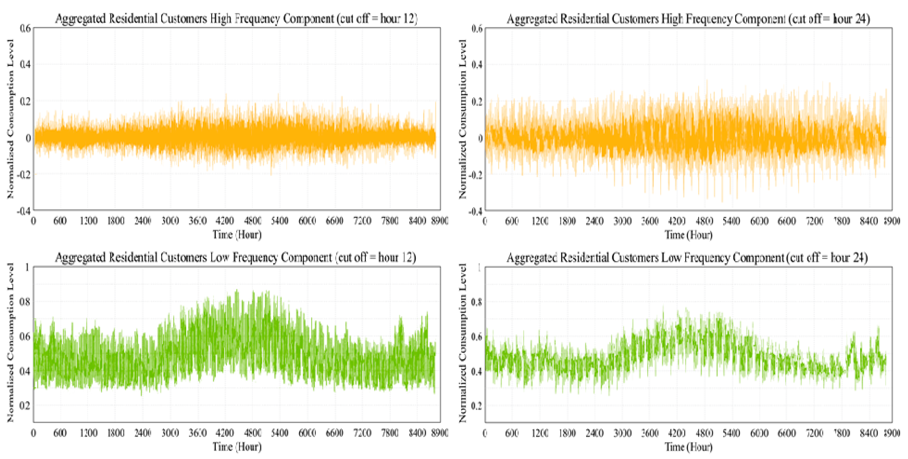
Figure 2 shows the time-domain signals of the aggregated residential customers. For aggregated residential customers, the high frequency components become almost double for a cut-off hour of 24, compared to a cut-off hour of 12. This pattern means that the amount of electricity consumed by activities with a frequency of 1–12 h is almost equal to the amount of electricity consumed by activities with a frequency of 13–24 h.

As shown in Figure 3, the share of high-frequency components is much higher than low-frequency components for individual residential customers. Residential customers, due to the diversity and spontaneity of their household activities, have highly fluctuating consumption signals.

Unlike industrial and commercial customers, the weekends do not have a major impact on the customers’ routines. This observation is very important, because typically, many load reduction calculation methods exclude weekends from their process. The exclusion of weekends is not necessary for residential customers.

The high-frequency components for a cut-off hour of 24 have a small increase compared to a cut-off hour of 12, which shows that most of the high-frequency activities of residential customers lie in the range of 1–12 h. Comparing the low and high frequency of the customer for a cut-off of hour 24, the low frequency is minimal compared to the high frequency. Therefore, we conclude that most residential activities have frequency ranges of less than 24 h. Spontaneity governs residential customers who typically do not follow schedules for their daily activities.

4.4. Predictability Analysis

An index is proposed to be used as a means for finding and quantifying similarity among the customers’ consumption signals. This index is called the predictability index and reflects the ratio of the low frequency components to the whole of the original consumption signal. The index is calculated by summing the share of high-frequency components and then subtracting the value from one, as shown in Equation (8):

$$P_{index}=1-\frac{{{\displaystyle \sum }}_{i=1}^{N}abs\left(c_i^{hf}\right)}{{{\displaystyle \sum }}_{i=1}^N{c}_i}$$

(8)

Table 1. P_index based on annual data for residential customers.

Cut off	Aggregated Residential	Individual Residential
Hour 12	0.9	0.44
Hour 24	0.85	0.36

Note: monthly and annual data provide almost identical results. For this reason, only annual values are listed.

shows a comparison between individual and aggregated residential demands. The randomness of individual residential customer demands makes it very difficult to estimate CBL accurately from the historical data of the customers. Mohajeryami [18], p. 54 shows that industrial and commercial predictability indexes are much higher than that for individual residential customers, but comparable to aggregated residential customers. However, aggregated residential customers show much higher predictability.

5. Data and Methodology

5.1. Data

We divide the data into four seasons to see the impact of seasonality. Seasons in Australia are as follows:

• Spring: September, October, and November.
• Summer: December, January, and February (note that since we have data for one year, January and February of that year precede December of that year, so the “summer” months are not consecutive).
• Fall: March, April, and May.
• Winter: June, July, and August.

The total consumption for all four seasons is depicted in Figure 4.

Residential customer household activities are diverse compared to large industrial and commercial customers, because many random parameters influence their electricity consumption. Due to the fact that randomness in electricity consumption is a main source of error in CBL calculation, irregular residential activities could adversely affect the DR performance. To improve the DR performance, we and others have proposed load aggregation, i.e., grouping customers into different clusters, to mitigate the randomness.

One proposed approach to improve performance is to use k-means clustering for assigning customers into different groups. Our novel k-means method uses the predictability index to aid the clustering. We will demonstrate that the customers’ P_index highly correlates with the CBL’s error performance. This correlation is significant for two reasons: first, we can use the P_index to demonstrate the upper limits of the error performance of the CBL calculation for each customer. Second, we can employ the P_index to cluster the customers into different groups, based on their error performance.

A few initial points must be randomly assigned to run a k-means algorithm. These points are called cluster centroids. The number of these points is determined based on the preferred number of clusters. K-means is an iterative algorithm. Its two primary functions are:

• Assigning a cluster;
• Moving the centroid to minimize an objective function.

Given a set of observations (x₁, x₂, ..., x_n), where each observation is a d-dimensional real vector, k-means clustering partitions the n observations into k (≤ n) sets S = {s₁, s₂, .., s_k}, so as to minimize the within-cluster sum of squares (WSS)—the sum of distance functions of each point in the cluster to the K center—shown in Equation (9):

$$\arg \underset{s}{\min }{\displaystyle \sum }_{i=1}^k{\displaystyle \sum }_{x\in S_i}||x-{\mu }_i{||}^2$$

(9)

We cluster customers based on their P_index values and simulated event-day average-hourly consumption. We select 12 simulated event days (one for each month) for the error analysis, shown in Figure 4 and

Table 2. Event Days in Sequence.

#	Event day	Season
1	Sept. 8th (252nd day)
2	Oct. 13th (287th day)	Spring
3	Nov. 25th (330th day)
4	Dec. 19th (354th day)
5	Jan. 30th (30th day)	Summer
6	Feb. 22nd (53rd day)
7	Mar. 18th (78th day)
8	Apr. 28th (119th day)	Fall
9	May 25th (147th day)
10	Jun. 23rd (175th day)
11	Jul. 28th (210th day)	Winter
12	Aug. 11th (224th day)

. The simulated event hours start at 3:00 p.m. and end at 9:00 p.m. Most of these days are high-use days that would be likely candidates for events for event days in an actual DR program.

K-means clustering is one of the unsupervised learning algorithms that partitions a given data set into a specified number of clusters (assume k clusters), fixed a priori. The “elbow criterion” is one way to select the number of clusters, but is not always unambiguous (the reference at the link shows two patterns, the first with a clear elbow, and the second without https://bl.ocks.org/rpgove/0060ff3b656618e9136b. Our pattern resembles the second). Figure 5 shows no obvious elbow. We decided to choose five cluster bins (k = 5).

There are many other ways to cluster the customers (Asadinejad et al. [19]); however, k-means clustering has proven to be very efficient. Figure 6 shows the results of the clustering.

We assigned customers into their respective bins with k-means clustering. For each bin, we compute the CBL for all customers and the average accuracy MAE. In columns 1 through 5 in

Table 3. The accuracy results of the California ISO (CAISO) customer baseline (CBL) calculation method.

Bin #	#Customers	Average Pindex	Accuracy MAE	Event-Day Average Consumption	MAE/Average
Bin 1	35	0.19	0.53	0.8	0.66
Bin 2	57	0.39	0.61	1.16	0.52
Bin 3	48	0.50	0.91	1.94	0.47
Bin 4	28	0.64	0.64	1.51	0.42
Bin 5	21	0.58	1.30	3.26	0.40
-	Correlation between Pindex and MAE/Average				−0.98

Note: CAISO uses Last10Days to determine baseline.

and

Table 4. The accuracy results of the Randomized Control Trial (RCT) CBL calculation method.

Bin #	#Customers	Average Pindex	Accuracy MAE	Event-Day Average Consumption	MAE/Average
Bin 1	35	0.19	0.75	0.80	0.94
Bin 2	57	0.39	0.87	1.16	0.74
Bin 3	48	0.50	1.16	1.94	0.60
Bin 4	28	0.64	1.00	1.51	0.66
Bin 5	21	0.58	2.18	3.26	0.67
-	Correlation between Pindex and MAE/Average				−0.88

Note: RCT aims to minimize the distance between the selected control group’s load curve and the load curve of DR participants. We perform the same analysis with the RCT method. The correlation between the P_index and the normalized accuracy MAE is −0.88; still a strong correlation, but not as high as clustering using the predictability index.

, we provide each bin’s number of customers, average P_index, CBL calculation’s accuracy MAE average, and the average hourly consumption. To show the relationship between the predictability index and the accuracy, we normalize each bin’s accuracy MAE by the event-day average hourly consumption for the 12 simulated event days. As shown in column 5, the average hourly consumption is different for the customers in each bin. Comparing the average accuracy MAE values of each bin (column 4) misleads without considering the difference in the average hourly consumption. Hence, we divide the value of accuracy MAE in column 4 by the value of the event-day average hourly consumption in column 5 for each bin. We calculate the normalized value and list it in column 6. As shown in Table 3, the normalized accuracy MAE (column 6) decreases (greater accuracy), as the average predictability index increases. The higher predictability index indicates that the CBL predicts more accurately. The correlation between the P_index and normalized MAE (MAE divided by the event-day average hourly consumption, using the 12 event days) is −0.98. The result reveals a robust relationship between the P_index value and the accuracy MAE of the CAISO CBL (Last10Days) calculation method.

Almost all research working on the evaluation, measurement, and verification (EM&V) of CBL calculation methods rely upon two metrics, accuracy and bias, to compare different CBL calculation methods. The strong correlation between the P_index and the normalized accuracy MAE suggests the possibility of using the P_index as an alternative or complement. Furthermore, we can use the P_index as a feature to demonstrate the limitation of the CBL calculation methods. If a customer’s index is low, no CBL calculation method is likely to work well. If the P_index is high without a satisfactory performance of the CBL method, then the method is likely to be inaccurate. A change in the CBL calculation method may be an effective way to improve error performance.

5.2. Results

5.2.1. Error Analysis before Using the Predictability Index

To examine how the load aggregation improves the error performance of CBL estimation, we initially applied a simple random load aggregation to the dataset. This part of the analysis analyzed the consumption data for 189 customers over 91 consecutive days, from October 1st to December 31st, 2012. We selected December 24th (Day 359) as a proxy for an event day, because that day constituted the maximum consumption in this partial dataset. The event hours start from 3:00 p.m. and end at 9:00 p.m.

Table 5. Error analysis before load aggregation.

CBL Method	MAE (kWh/hr)	Bias (kWh/hr)	OPI (kWh/hr)
NYISO	1.1923	−0.0436	0.6179
Adjusted NYISO	1.4396	0.3294	0.8845
ISO-NE	1.0656	−0.4552	0.7604
Adjusted ISO-NE	1.1814	0.1846	0.6830
Regression	1.3341	−0.6232	0.9786
Adjusted Regression	1.3591	0.1961	0.7776

Note: NYISO uses High4of5. ISO-NE uses exponential smoothing, with a weighting factor of 90% for the previous day’s CBL and 10% for the current day’s consumption. Note also applies to Table 6. The results use 91 consecutive days, from October 1 through December 31, 2012.

applies the three metrics to the CBL calculations and their (additively) adjusted forms before load aggregation. The calculated values are for event hours of 3 p.m. to 9 p.m. According to the results, the morning adjustment reduces the accuracy of each CBL method. However, for OPI values, the adjustment improved the results substantially for ISO-NE and regression methods. The adjustment did not improve the OPI of NYISO.

5.2.2. Error Analysis after Random Load Aggregation

We next apply a random load aggregation to the sample data, to examine whether load aggregation and random clustering improve the accuracy, bias, and OPI values of CBL calculation methods provided in

Table 6. Accuracy, bias and overall performance index (OPI) for clustered methods at event hours.

Clustered Method	Accuracy MAE (kWh/hr)	Bias (kWh/hr)	OPI (kWh/hr)
Clustered NYISO	0.6808	−0.2256	0.4532
Adjusted Clustered NYISO	0.7439	0.2988	0.5213
Clustered ISO-NE	0.6846	−0.4571	0.5708
Adjusted Clustered ISO-NE	0.6172	0.1935	0.4053
Clustered Regression	0.9074	−0.6611	0.7842
Adjusted Clustered Regression	0.6921	0.1901	0.4411

.

Figure 7 shows that simple load aggregation and clustering clearly improves accuracy, while leaving bias unaffected. The additive same-day adjustment generally has a positive effect on accuracy. NYISO is the exception.

Table 7. Sensitivity analysis of number of customers in each cluster’s impact on overall performance index.

No. of Clusters (No. of Customers)	Overall Performance Index (kWh/hour)
	NYISO	ISO-NE	Regression
2 (100)	0.3704	0.4593	0.6385
4 (50)	0.3514	0.4609	0.6356
5 (40)	0.3597	0.4722	0.6524
8 (25)	0.3645	0.4854	0.6616
10 (20)	0.3840	0.5008	0.6891
20 (10)	0.4140	0.5257	0.7161
25 (8)	0.4088	0.5288	0.7802
40 (5)	0.4532	0.5708	0.7842
50 (4)	0.4779	0.5979	0.8161
100 (2)	0.5314	0.6636	0.8631
No Cluster	0.6179	0.7604	0.9786

shows the sensitivity of OPI to the number of clusters. As the number of customers in each cluster increases, the OPI generally improves accordingly for all three methods. According to the results, even grouping two customers in a cluster can improve OPI by 13.99%, 12.73%, and 11.80% for the NYISO, ISONE and regression method, respectively. These values generally increase as the number of customers in each cluster increases, except for the case of two clusters with 100 customers per cluster.

5.2.3. Error Analysis for the Proposed CBL Estimation Method

We now apply the proposed CBL estimation method to the dataset. After obtaining all predictability indices and applying k-means clustering, the data is organized into five bins (k = 5), as was shown in Figure 6. Visual inspection suggests that customers in bins 4 and 5 have the highest variability. Bin 1 has the lowest variability. Actual variability is based upon box plots shown in Appendix A, Figure A1, obtained for each season from the aggregated data for each bin. Although different seasons have slight variations, the overall patterns are similar. And while customers might vary behavior over time, individual residential customers follow similar patterns, most of the time. The loads show the highest variability during noontime.

Next, we estimate the CBL for each group and calculate the error performance. We utilize two CBL methods, CAISO and PJM.

Table 8. MAE for CAISO method.

Bin	k = 1	k = 2	k = 3	k = 4	k = 5	k = 6	k = 7	k = 8	k = 9	k = 10
1	1.201	0.904	0.760	0.679	0.685	0.563	0.615	0.482	0.576	0.551
2	0.621	0.467	0.432	0.338	0.366	0.342	0.248	0.324	0.303	0.286
3	0.819	0.671	0.558	0.531	0.493	0.463	0.449	0.429	0.411	0.395
4	0.723	0.607	0.541	0.483	0.396	0.432	0.323	0.397	0.368	0.373
5	1.727	1.400	1.011	1.111	1.060	0.989	0.605	0.930	0.896	0.868

Notes: CAISO uses the Last10Days method to calculate the baseline. In Table 8 and Table 9, k indicates number of customers (randomly selected) in a group within each bin; k=1 indicates no cluster. The results shown in the tables are average values from results obtained using five (5) random combinations of customers.

lists the error performance results for the CAISO method.

Table 9. MAE for PJM method.

Bin	k = 1	k = 2	k = 3	k = 4	k = 5	k = 6	k = 7	k = 8	k = 9	k = 10
1	1.170	0.878	0.739	0.654	0.669	0.533	0.584	0.457	0.554	0.537
2	0.640	0.460	0.462	0.337	0.385	0.354	0.244	0.326	0.315	0.300
3	0.801	0.661	0.556	0.531	0.501	0.479	0.458	0.424	0.426	0.395
4	0.712	0.613	0.544	0.490	0.378	0.426	0.313	0.409	0.377	0.381
5	1.718	1.407	0.992	1.160	1.084	0.971	0.566	0.925	0.920	0.932

Note: PJM uses the High4of5 method to calculate the baseline.

lists the error results for the PJM method. These results show an average of MAE for all 12 events. We ran five random combinations of customers in each bin and then averaged the MAE, so as to remove the possibility that the results were specific to a single random draw. For example, Bin #1 has 35 customers. For the entry k = 2, 17 (35/2), groups of two customers are created five times randomly. Results of the five random combinations are averaged and shown in Table 8 and Table 9. In this case, because 17 × 2 = 34, information from one customer (35 – 34 = 1) is not used in each of the five combinations (not necessarily the same customer).

For both CAISO and PJM, MAE tends to decrease as the number of customers in a cluster increases. In CAISO, we observed the largest decrease in MAE in bin 1 of 54.122% and the smallest decrease in bin 4 of 48.409%. We found similar effects in PJM, with the largest MAE decrease in bin 1 of 54.103% and the smallest decrease in bin 5 of 45.751%. The decrease is larger for the less variable bins and smaller for the more variable bins.

The bias is not sensitive to the number of customers in a cluster. There seems to be no relationship between the bin’s variability and the bias value. Appendix B,

Table A1. Bias value for CAISO method.

Bin	k = 1	k = 2	k = 3	k = 4	k = 5	k = 6	k = 7	k = 8	k = 9	k = 10
1	−0.255	−0.233	−0.249	−0.239	−0.26	−0.218	−0.26	−0.193	−0.255	−0.255
2	−0.064	−0.065	−0.062	−0.058	−0.058	−0.058	−0.043	−0.060	−0.064	−0.064
3	−0.156	−0.157	−0.151	−0.156	−0.159	−0.156	−0.154	−0.153	−0.156	−0.156
4	−0.103	−0.104	−0.103	−0.106	−0.089	−0.11	−0.079	−0.104	−0.103	−0.103
5	−0.488	−0.484	−0.400	−0.481	−0.491	−0.487	−0.387	−0.465	−0.488	−0.488

and

Table A2. Bias value for PJM method.

Bin	k = 1	k = 2	k = 3	k = 4	k = 5	k = 6	k = 7	k = 8	k = 9	k = 10
1	−0.256	−0.241	−0.237	−0.210	−0.256	−0.241	−0.256	−0.226	−0.256	−0.256
2	−0.071	−0.058	−0.071	−0.066	−0.071	−0.071	−0.052	−0.071	−0.071	−0.071
3	−0.154	−0.154	−0.148	−0.154	−0.154	−0.154	−0.154	−0.154	−0.154	−0.154
4	−0.105	−0.105	−0.105	−0.105	−0.085	−0.105	−0.075	−0.105	−0.105	−0.105
5	−0.532	−0.532	−0.442	−0.532	−0.532	−0.532	−0.413	−0.532	−0.532	−0.532

, contain the bias values for CAISO and PJM.

5.2.4. Comparing the Predictability Method with Random Load Aggregation

The predictability approach improves upon random load aggregation. Although random load aggregation considerably improved the error performance of CBL estimation methods, our method further improves demand response calculations.

Table 10. MAE for simple load aggregation and the predictability method for CAISO and PJM CBL estimation methods.

-		k (Number of Customers in a Cluster)
		1	2	3	4	5	6	7	8	9	10
CAISO	Simple load aggregation	1.01	0.83	0.68	0.64	0.58	0.56	0.52	0.51	0.52	0.52
	Predictability method	1.01	0.81	0.66	0.62	0.60	0.55	0.44	0.51	0.51	0.49
PJM	Simple load aggregation	1.00	0.83	0.73	0.66	0.62	0.58	0.54	0.53	0.52	0.49
	Predictability method	1.00	0.77	0.64	0.59	0.55	0.47	0.41	0.42	0.43	0.42

Note: CAISO uses Last10Days, while PJM uses Highest 4of5.

lists the results of both random load aggregation and the predictability method for CAISO and PJM.

According to Table 10 for CAISO, the average accuracy MAE for all k’s using random aggregation and the predictability method are 0.601 and 0.58. This results in a 3.43 percent improvement in MAE accuracy with our approach. For PJM, the average MAE accuracy for all k’s for random aggregation and the predictability method are 0.616 and 0.527, which is equivalent to a 14.42 percent improvement. The improvement is larger for PJM; the combined effect of the load aggregation and the clustering, based on the predictability index, causes this improvement. If the proposed clustering method, based on the predictability index, incurs a large administrative cost, random aggregation still achieves a significant improvement. In large DR programs, where even a small improvement in accuracy can translate into a significant financial gain, clustering will be beneficial.

6. Conclusions

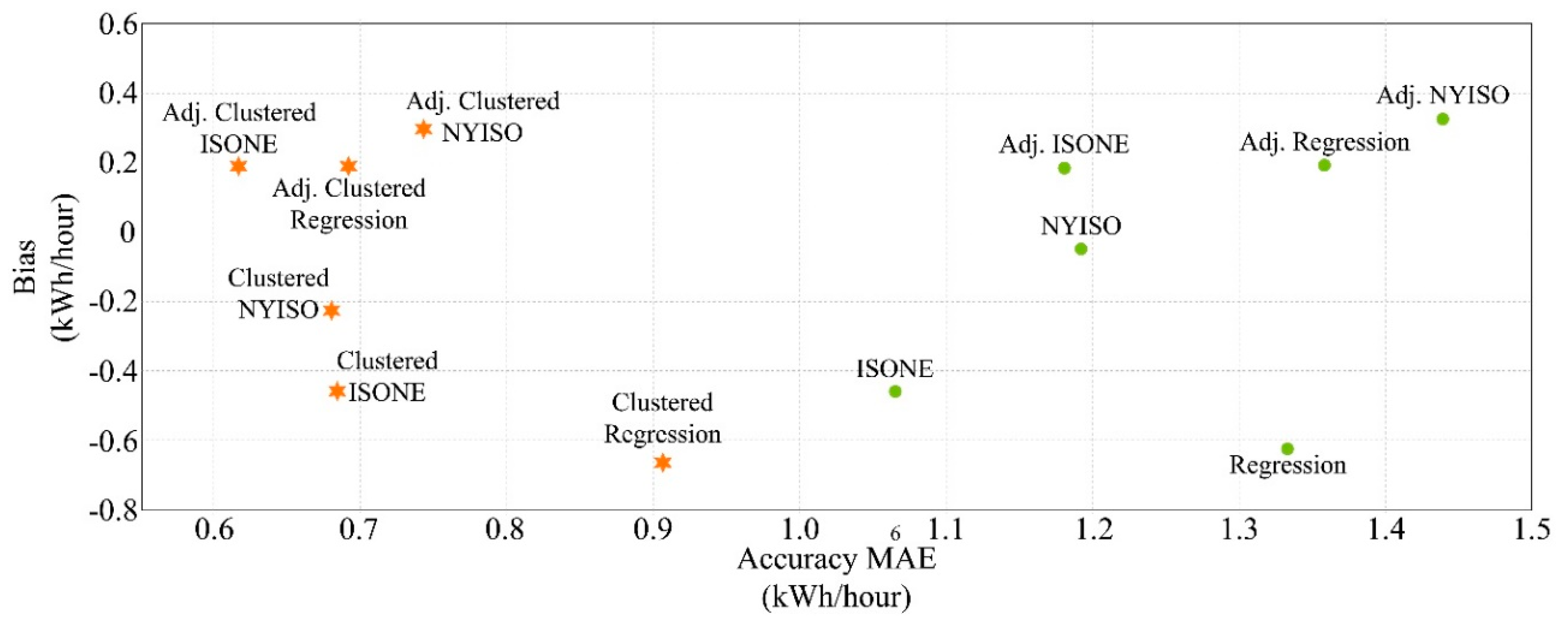
Demand response programs need reliable evaluation, measurement, and verification (EM&V) methods. One of the major EM&V challenges in DR programs is an accurate estimation of the load reduction, particularly for residential customers who show large stochasticity. To ascertain the load reduction for residential DR programs, it is essential to estimate the customer baseline load (CBL) accurately. The necessity of CBL calculation introduces several challenges to DR programs, including random variations in demand and heterogeneous patterns. To address these challenges, we propose k-means clustering based on demand size and predictability. We first show the theoretical merits of this proposed method. We then provide an empirical analysis of residential customers from an Australian electricity provider, showing that clustering customers according to size and predictability improves the error performance. The improvement over random clustering ranges from approximately 3% to 14%, with larger increases compared to no clustering.

The new predictability clustering method provides a meaningful improvement to random clustering. The method produces a lower mean average error (MAE), indicating higher accuracy and better capacity predictions. Our method found a strong correlation between MAE and predictability.

We also consider demand variability. Variability increases MAE. Larger group sizes produce lower MAE, but the decrease is largest for the cluster with the least variability and smallest for the one with greatest variability.

Overestimation and underestimation, and positive and negative bias, respectively, either over- or under- compensate customers. Neither the number of customers in the bin, nor their variability, had a noticeable impact on bias.

Future work can explore alternative methods. Wavelet transform (WT) offers the more robust handling of time-domain data with variable frequency. WT decomposes signals into a set of functions, containing expansions, contractions, and transitions of a single primary function, referred to as a wavelet. The greater division of frequencies can create a higher resolution for analysis, potentially increasing accuracy. Combining predictability methods with randomized controlled trial (RCT) may increase the accuracy of RCT, requiring a less administratively burdensome data set for predictability methods.

Larger data sets should achieve higher levels of predictability and accuracy. If more detailed customer data are available, characteristics such as income, education, and household size may affect predictability. To further increase accuracy, further research can align customer characteristics with predictability assumptions, to decrease error and detect correlations with the size-predictability index.

Actual DR programs likely maintain the information necessary to test the theory. These data will allow one to test CBL accuracy, as well as the revenue of the utility. The successful implementation and development of predictability methods warrants the theory be tested in a variety of conditions, such as differing climates and differing electricity market structures. In particular, actual DR programs can provide the opportunity to minimize the effects of customer stochasticity, so as to avoid “paying for nothing.”

References

1. Bushnell, J.; Hobbs, B.F.; Wolak, F.A. When It Comes to Demand Response, Is FERC Its Own Worst Enemy? Electr. J. 2009, 22, 9–18. [Google Scholar] [CrossRef] [Green Version]
2. Borenstein, S. Wealth Transfers Among Large Customers from Implementing Real-Time Retail Electricity Pricing. Energy J. 2007, 28, 131–150. [Google Scholar] [CrossRef]
3. Faruqui, A.; Sergici, S. Dynamic pricing of electricity in the mid-Atlantic region: Econometric results from the Baltimore gas and electric company experiment. J. Regul. Econ. 2011, 40, 82–109. [Google Scholar] [CrossRef]
4. Gneezy, U.; Meier, S.; Rey-Biel, P. When and Why Incentives (Don’t) Work to Modify Behavior. J. Econ. Perspect. 2011, 25, 191–210. [Google Scholar] [CrossRef] [Green Version]
5. Williamson, C.; Marrin, K. Peak Time Rebate’s Dirty Little Secret. Energy Insights 2009. [Google Scholar]
6. Supreme Court of the United States (SCOTUS). Federal Energy Regulatory Commission vs. Electric Power Supply Association, Docket No. 14-840. 2016. Available online: https://www.supremecourt.gov/opinions/15pdf/14-840-%20new_o75q.pdf (accessed on 7 February 2020).
7. Zhang, Y.; Chen, W.; Xu, R.; Black, J. A Cluster-Based Method for Calculating Baselines for Residential Loads. IEEE Trans. Smart Grid 2015, 7, 2368–2377. [Google Scholar] [CrossRef]
8. Navigant. Market Data: Residential Demand Response. Available online: https://www.navigantresearch.com/reports/market-data-residential-demand-response (accessed on 27 March 2020).
9. Mohajeryami, S.; Cecchi, V. An investigation of the Randomized Controlled Trial (RCT) method as a Customer Baseline Load (CBL) calculation for residential customers. In Proceedings of the 2017 IEEE Power & Energy Society General Meeting, Chicago, IL, USA, 16–20 July 2017; pp. 1–5. [Google Scholar]
10. Australian Energy Market Operator (AEMO). Electricity Load Profiles. n.d. Available online: http://www.aemo.com.au/Electricity/National-Electricity-Market-NEM/Data/Metering/Load-Profiles (accessed on 7 February 2020).
11. Goldberg, M.; Agnew, G. Protocol Development for Demand Response Calculation–Findings and Recommendations; Report CEC 400-02-017F; California Energy Commission: Sacramento, CA, USA, 2003.
12. Pepco, District Customers Respond to Smart Grid Pricing. 2010. Available online: https://www.pepco.com/News/Pages/2010-09-09.aspx (accessed on 27 March 2020).
13. AEE Institute, Maryland’s Demand Response Program–Baltimore Gas & Electric’s Smartenergy Rewards 2019. Available online: https://info.aee.net/hubfs/MD%20DR%20Final.pdf (accessed on 7 February 2020).
14. Wijaya, T.K.; Vasirani, M.; Aberer, K. When Bias Matters: An Economic Assessment of Demand Response Baselines for Residential Customers. IEEE Trans. Smart Grid 2014, 5, 1755–1763. [Google Scholar] [CrossRef]
15. Jazaeri, J.; Alpcan, T.; Gordon, R.; Brandao, M.; Hoban, T.; Seeling, C. Baseline methodologies for small scale residential demand response. In Proceedings of the 2016 IEEE Innovative Smart Grid Technologies—Asia (ISGT-Asia), Melbourne, Australia, 28 November–1 December 2016; pp. 747–752. [Google Scholar]
16. Hatton, L.; Charpentier, P.; Matzner-Lober, E. Statistical Estimation of the Residential Baseline. IEEE Trans. Power Syst. 2015, 31, 1752–1759. [Google Scholar] [CrossRef]
17. Mohajeryami, S.; Doostan, M.; Asadinejad, A.; Schwarz, P. Error Analysis of Customer Baseline Load (CBL) Calculation Methods for Residential Customers. IEEE Trans. Ind. Appl. 2017, 53, 5–14. [Google Scholar] [CrossRef]
18. Mohajeryami, S. An Investigation of the Impact of Customer Baseline (CBL) Calculation on Peak Time Rebate Program. Ph.D. Thesis, UNC Charlotte, Charlotte, NC, USA, 2016. [Google Scholar]
19. Asadinejad, A.; Varzaneh, M.G.; Tomsovic, K.; Chen, C.; Sawhney, R. Residential customers elasticity estimation and clustering based on their contribution at incentive based demand response. In Proceedings of the 2016 IEEE Power and Energy Society General Meeting (PESGM), Boston, MA, USA, 17–21 July 2016. [Google Scholar]
Figure 1. (a) Low pass filter, and (b) high pass filter.
Electronics 09 00570 g001
Figure 2. Time-domain electricity consumption signals for aggregated residential customers.
Electronics 09 00570 g002
Figure 3. Time-domain electricity consumption signals for individual residential customers.
Electronics 09 00570 g003
Figure 4. Total daily consumption dataset for Australian Energy Market (AEMO) for 189 residential customers, 2012.
Electronics 09 00570 g004
Figure 5. Elbow criterion analysis.
Electronics 09 00570 g005
Figure 6. The relationship between average consumption level and predictability index.
Electronics 09 00570 g006
Figure 7. CBL method accuracy and bias for event hours.
Electronics 09 00570 g007