Article

Density Peak Clustering Algorithm Considering Topological Features

1
School of Information Science and Engineering, Shandong Normal University, Jinan 250358, China
2
School of Light Industry Science and Engineering, Qilu University of Technology (Shandong Academy of Sciences), Jinan 250351, China
3
Department of Electrical Engineering and Information Technology, Shandong University of Science and Technology, Jinan 250031, China
*
Authors to whom correspondence should be addressed.
Electronics 2020, 9(3), 459; https://doi.org/10.3390/electronics9030459
Submission received: 18 January 2020 / Revised: 5 March 2020 / Accepted: 6 March 2020 / Published: 8 March 2020
(This article belongs to the Section Computer Science & Engineering)

Abstract

:
The clustering algorithm plays an important role in data mining and image processing. The breakthrough of algorithm precision and method directly affects the direction and progress of the following research. At present, types of clustering algorithms are mainly divided into hierarchical, density-based, grid-based and model-based ones. This paper mainly studies the Clustering by Fast Search and Find of Density Peaks (CFSFDP) algorithm, which is a new clustering method based on density. The algorithm has the characteristics of no iterative process, few parameters and high precision. However, we found that the clustering algorithm did not consider the original topological characteristics of the data. We also found that the clustering data is similar to the social network nodes mentioned in DeepWalk, which satisfied power-law distribution. In this study, we tried to consider the topological characteristics of the graph in the clustering algorithm. Based on previous studies, we propose a clustering algorithm that adds the topological characteristics of original data on the basis of the CFSFDP algorithm. Our experimental results show that the clustering algorithm with topological features significantly improves the clustering effect and proves that the addition of topological features is effective and feasible.

1. Introduction

With the advent of the era of big data, information grows rapidly [1,2]. The influx of massive data makes the statistics and screening of important information more difficult. Cluster analysis is an important statistical analysis method, which is mainly used to solve classification problems. It is a technique for integrating similar information into meaningful subclasses of data and trying to find patterns embedded in the underlying structure of massive data [3,4,5]. Cluster analysis has been widely used in computer vision, database knowledge discovery, image processing and other fields [6,7,8,9]. Due to its wide applicability, many clustering algorithms have been invented, including K-means, the Affinity Propagation (AP) algorithm, Density-Based Spatial Clustering of Applications with Noise (DBSCAN), Ordering Points to Identify the Clustering Structure (OPTICS) and the Clustering by Fast Search and Find of Density Peaks (CFSFDP) algorithm [9,10]. Although these methods solve many data clustering problems, they also have their own limitations and disadvantages. Therefore, with the increase in data complexity and the study of clustering methods, the improvement and expansion of classical methods have become the mainstream research direction. Below, we will introduce the advantages and disadvantages of the above clustering algorithms.
The K-means algorithm is an algorithm that adopts the alternative minimization method to solve non-convex optimization problems [11,12] and it is a representative of the prototype-based clustering method of objective functions. It divides a given data set into K clusters designated by users and has a high execution efficiency. However, the K-means algorithm needs to specify the number of clustering centers in advance. Different K values have a great impact on the experimental results and, in the actual operation, multiple attempts are required to obtain the optimal K value. Firstly, the objectivity of the K value makes the clustering results mostly different. Secondly, this algorithm is not friendly to non-convex data sets and it is difficult to obtain satisfactory clustering results.
The AP clustering algorithm [13,14] is an unsupervised clustering algorithm. The algorithm realizes the clustering process through the interaction between data points. The advantages of the algorithm are that there is no need to define the number of classes in advance, the clustering center can be obtained adaptively through the iterative process, and the location and number of class centers can be identified automatically from the data points, so as to maximize the similarity sum of all similar points. At the same time, the algorithm has disadvantages. Since the AP algorithm needs to calculate the similarity between each pair of data objects in advance, when there are many data objects, the memory footprint will be high. Moreover, its high time complexity O(N3) is one of its shortcomings.
The DBSCAN algorithm [15,16] is a clustering algorithm based on data point density. It gets rid of the constraint of data set shape requirement and can obtain class clusters of arbitrary shapes. The DBSCAN algorithm needs to establish an appropriate density threshold, and points with a density greater than this threshold become “core points”; it then aggregates all points within the threshold into the same class. The advantage of this algorithm is that the number of clustering centers does not need to be determined in advance, and noise points and outliers can be eliminated well. However, DBSCAN also has deficiencies. When the density of sample sets is not uniform and the clustering spacing is greatly different, the clustering quality is poor, which is mainly caused by the limitations of distance threshold and density threshold. Generally, the determination of these two parameters depends on the researcher’s experience, which also leads to the limitation of the algorithm.
The OPTICS algorithm [17] is an improved version of DBSCAN, so the OPTICS algorithm is also a density-based clustering algorithm. In DBCSAN, algorithms need to input two parameters: the ϵ (distance threshold) and MinPts (density threshold). Choosing different parameters will lead to the final clustering result difference being very big; therefore, DBCSAN is too sensitive for the input parameters. OPTICS is proposed to help the DBSCAN algorithm select appropriate parameters and reduce the sensitivity of input parameters. This mainly aims at the improvement of too sensitive input parameters, e.g., the input parameters of DBSCAN (ϵ and MinPts). Although OPTICS also needs two inputs, the algorithm is not sensitive to ϵ input (generally, ϵ is fixed as infinity); at the same time, the algorithm does not explicitly generate data clustering, it just sorts the objects in the collection of data, gets an ordered list of objects, through which an ordered list can be compiled in order to get a decision diagram and, via this decision diagram, the algorithm can cluster data sets to different ϵ parameters. First, these are obtained by the fixed MinPts and infinite ϵ ordered list, then a decision diagram is created, by which the clustering of data is achieved when ϵ takes specific value.
CFSFDP is a new clustering algorithm based on density. The algorithm has a lot of bright spots; for example, it can discover clusters of arbitrary shape, it needs less parameters and samples, no iterative classification, non-equilibrium data sets (where the number of points in different clusters varies greatly) can be well processed, and its performance is better in large-scale data sets. However, there are some shortcomings. The algorithm has two important parameters, local density and cut-off distance. The choice of cut-off distance directly affects the accuracy of the clustering results, and the algorithm ignores the topological relationship between the data.
Since the emergence of Word2vec, many fields can use its ideas for embedding. The Item2vec algorithm based on item sequence is adopted. Graph embedding technology is based on graph structure. The DeepWalk method in graph embedding takes the node sequence obtained by random walk as a sentence, obtains part of the network information from the truncated random walk sequence, and then learns the potential representation of nodes through part of the information—that is, the topology characteristics. In order to solve the problem that the CFSFDP algorithm does not consider the topological characteristics of data, we innovatively proposed a new idea, using DeepWalk algorithm to represent the potential information of data, and applying this representation as topological characteristics to data clustering to improve the accuracy of data clustering. The general process is shown in Figure 1.
On the basis of the CFSFDP algorithm, we chose to combine the topological features obtained by the DeepWalk algorithm to invent a new clustering algorithm. As far as we know, there are few studies on the combination of topological features and clustering algorithms, mainly because topological features are not easy to obtain. We have deftly applied the DeepWalk approach to social characteristics to solve this problem. Our motivation is twofold: 1) solve the problem of difficult topology feature acquisition; 2) improve the clustering precision by combining topology features with the CFSFDP clustering algorithm.

2. DPCTF Algorithm

The algorithm is based on the CFSFDP algorithm and DeepWalk [7]. This method is based on previous theories and topological features. This section briefly reviews the CFSFDP, DeepWalk and topological characteristics.

2.1. Clustering by Fast Search and Find of Density Peaks

CFSFDP is a clustering algorithm based on density peak. The core idea is to calculate the relative density and the nearest distance through the cut-off distance, draw the decision graph by using the absolute density and the nearest distance, and subjectively select the clustering center point on the decision graph to achieve the data clustering [18,19].
When performing clustering, the CFSFDP algorithm first needs to determine the center point of the class. It assumes that the local density of the clustering center of the cluster is higher than that of the surrounding data points, and the distance between the clustering center and those data points with a higher local density is larger. For a given data set, the CFSFDP algorithm needs to calculate two quantization values for each data point: the value of the local density ρ i of the data point and the distance from the data point whose local density is higher than its δ i .
The local density ρ i of data point x i has two calculation methods: The cutoff distance kernel method and a method based on the Gaussian kernel computing method. The procedure of calculating the local density formula by cutoff distance kernel is to use the absolute distance between data points to subtract the cutoff distance. If the result is less than zero; that is, if the distance between data points is less than the preset cutoff distance, the function takes one, otherwise the result is zero. In the formula for ρ i = j χ ( δ i j d c ) , where χ ( x ) = {   0 , x > 0 1 , x 0 , δ i j is the distance between data, d c is the cutoff distance. The local density ρ i of the data point obtained with this calculation method usually equals the number of data points with a distance less than d c around the data point. In fact, the greater the number of points which are closer to x i than d c , the greater the density.
The method based on the Gaussian kernel computing method often uses high-dimensional cluster data. The main idea of the kernel clustering method is to map the data points in the input space to the high-dimensional characteristic space through nonlinear mapping, and select an appropriate Mercer kernel function to replace the inner product of the nonlinear mapping to carry out clustering in the characteristic space. This increases the probability of linearly separable data points through nonlinear mapping; that is, it can better distinguish, extract and amplify useful features, so as to achieve more accurate clustering, and the algorithm has a faster convergence speed. Gaussian kernel clustering is the mapping of data points in data space to a high-dimensional feature space. Then, a sphere with the smallest radius can be found in the feature space to cover all data points, and the sphere is mapped back to the data space to obtain the set of contour lines containing all data points. These contour lines are the boundaries of the cluster. Each point surrounded by a closed contour line belongs to the same cluster. The difference between calculating local density with the cutoff kernel and Gaussian kernel is that the former results in a discrete value and the latter in a continuous value.
Distance δ i between data points is obtained by calculating the distance between data point x i and other data points with higher local densities than this data point. The distance δ i between data points can be calculated according to Formula (1).
δ i = {   max ( δ i j ) , ρ j ρ i min ( δ i j ) , ρ j > ρ i
δ i is measured by computing the minimum distance between the point i and any other point with higher density and for the point with highest density, use δ i = max ( δ i j ) .
The two-dimensional decision graph is established by using ρ i and δ i , as shown in Figure 2.
After calculating the ρ i and δ i of each point, the two attributes are used as the coordinate axes to generate the decision graph as shown in the Figure 2. In the decision graph, the points with larger ρ i and δ i are manually selected as the center points of the class cluster. The literature also suggests a formula, λ i = ρ i δ i , to better select the clustering center. The closer the point is to the upper right corner of the decision graph, the greater the λ i value after calculation by the formula.
After all the class cluster centers are selected, the CFSFDP algorithm allocates the remaining points to the cluster where the local density is greater than it and the point closest to it is located.
The flow of the algorithm is shown in the following steps:
Step 1: preset the distance threshold d c and the local density ρ i of each point is calculated;
Step 2: Sort density points from high to low;
Step 3: Let δ 1 = max j ( d j ) , calculate δ i according to formula (1), and store the corresponding label;
Step 4: Make a decision graph based on the parameters δ i and ρ i , and select the center point of the cluster;
Step 5: According to the cluster center point, data object label and density boundary threshold, the remaining points are divided into each cluster or boundary region.

2.2. DeepWalk

DeepWalk is the earliest node vecturization model based on Word2vec [20], which maps every node in a network to a low-dimensional vector. To put it simply, DeepWalk uses a vector to represent each node in the network and expects these vectors to express the relationships among the nodes in the network; that is, the more closely related the nodes in the original network are, the closer the corresponding vectors are in their space. The main idea is to imitate the Word2vec text generation process by constructing the random walk path of nodes on the network. According to the sequence of nodes generated by the random walk [21,22,23], the Skipgram and Hierarchical Softmax models [24] are used to model the probability of nodes in the random walk sequence, maximize the probability of node occurrence in the random walk sequence and, finally, use the process of random gradient descent to learn the parameters.
DeepWalk takes the graph as input to generate a potential representation as output. Applying this method to the Karate Club network, the result is shown in Figure 3. Figure 3a shows the layout of the Karate Club data. Figure 3b shows the distribution of the two potential dimension outputs by DeepWalk in the coordinate system. We observed that the distribution of data points in Figure 3b was similar to that of the original data points, but there were also linearly separable parts. This finding can help with data clustering.
The following steps describe this algorithm procedure:
Input: network/graph;
Import data into random walk to obtain node representation mapping;
Import the node sequence into Skipgram update model, map the node to its current representation vector Φ ( v j ) and use the stochastic gradient descent algorithm to maximize the probability of all words appearing in the context;
Output: representation.

2.2.1. Random Walk Generator

The so-called random walk method is used to select random walk paths repeatedly in the network and eventually form a path through the network. Starting at a particular endpoint, each step of the walk randomly selects one of the edges connected to the current node, then moves along the selected edge to the next vertex, and so on.
Random walk obtains the local information of the network from the truncated random walk sequence and uses it to learn the vector representation of nodes, which makes it is easy to parallelize. When the network structure has a slight change, a new random walk can be generated for the changing part to update the learning model and improve the learning efficiency. If the nodes of a network follow the power-law distribution, the number of occurrences of the nodes in the random walk sequence should also follow the power-law distribution.

2.2.2. Skipgram

Skipgram is an implementation method for the vector representation of text in Word2vec. It is a kind of neural probability language model. The main idea of Skipgram is to use words to predict sentences. The context of a sentence consists of the words in the left and right Windows of a given word, and the window size is artificially set. The Skipgram language model requires the maximization of the probability of words appearing in the context. In other words, Skipgram achieves the representation of the characteristics of words. In DeepWalk, the author applies the vector representation of text in Word2vec to the social network relations, and indicates that, as long as the data types satisfy the power-law distribution, the vector representation of nodes can be realized by this method. According to this idea, we also carry out vector representation of clustering data nodes.

2.3. Topological Structure

Topological relation [25,26,27,28] is a geometric concept, which includes the relation of adjacency, association, inclusion and connection among points, lines and planes. This concept is extended to image processing. Topological structure is one of the basic properties of image, which often contains more accurate image information than simple feature points, such as corner points and inflection points. Topology is the property of a graph that remains unchanged after topological transformation. For example, as shown in the figure below, Figure 4 is a rectangular plane with large mass. There is a point X in the plane. After two-dimensional topological transformation (stretching and compression) of the rectangle, the length, width and height of the rectangle all change, and the ratio also changes. Thus, this built-in property that point X is inside the rectangle, is called a topological property or a topological feature [29,30,31,32].
Topological structure plays an important role in image segmentation and classification, but it is not widely used in data clustering, which makes it a research blank for combining topological structure information with clustering algorithm. In this paper, topological characteristics and a clustering algorithm are combined to achieve the purpose of improving clustering results.

2.4. Density Peak Clustering Algorithm Considering Topological Features

The CFSFDP algorithm still has some flaws. When the CFSFDP algorithm is used to process the data set, it is found that the clustering effect is not ideal in practical applications, and the main reason for this problem may be the selection of the data set and cutoff distance [33,34,35]. By summarizing and thinking about the classical clustering algorithm, we find that the classical clustering algorithm does not consider the topological characteristics of the data set. Therefore, in order to verify the effect of topology on clustering effect, the following experimental scheme was proposed. The specific operation process is shown in Figure 5.
As an important feature of graphs, topological features play an important role in image processing; for example, topologies are often introduced when drawing satellite maps [36,37,38,39,40,41,42,43]. However, in the field of clustering research, topological features are rarely applied. Therefore, we take the lead in proposing a clustering algorithm based on topological characteristics, We call it Density Peak Clustering Algorithm Considering Topological Features (DPCTF).
First, we need to analyze and preprocess the original data. As can be seen from Figure 6, the original data is the commonly used form of point setting in the clustering algorithm, and the topological structure of the data is not considered. We transform the original data to graph form with the topological structure by finding the connection between data points.
Through analysis of the original data, it is found that the data contains three features. The first feature is the initial data point, the second feature is all data points except the initial feature point, and the third feature is the distance between feature one and feature two. We processed the original data according to feature three and obtained the topology structure of the original data points.
Through the analysis of characteristics, we found that there is a certain rule for the distance between points. By summarizing the rule, we selected data with the distance less than γ to connect ( γ is a distance threshold value; throughout the test, we used γ = 0.35 to achieve the best experimental effect), so as to form a topological relationship. The resulting data contains the following information.
The information in each row represents the topological relationship between this data point and all other connectable data points.
All connectable data points are points that meet the preset conditions.
After we preprocessed the original data, we obtained the topology of the original data. Through this topology, we obtained the input form required by DeepWalk, imported the graph obtained in the previous step into DeepWalk, and obtained the topological characteristics of the graph through the random walk and Skipgram in DeepWalk. It is important to note here that DeepWalk’s output feature dimensions are adjustable and theoretically unconstrained, but the original suggests choosing multiples of four, where we tried one and four dimensions (to prevent the results from being too high). From the results, we found that for the data we processed, the one-dimensional feature was more effective.
After obtaining the output of DeepWalk, we combined the topological features obtained with the original data one by one. One can obtain new data in a higher dimension. We called this data the cluster data set, considering its topological characteristics. We put this new data set it into the CFSFDP algorithm to verify the clustering effect.
J m = i = 1 N j = 1 C u i j m x i c j 2
u i j = 1 k = 1 C ( x i c j x i c k ) 2 m 1   ,   c j = i = 1 N u i j m · x i i = 1 N u i j m
First, we used the Density Peak Clustering Algorithm to perform rough clustering of the data; in order to obtain the number of class clusters m ; i , j are the class labels, where i represents the i th sample and j represents the j th cluster. Topological features are used as weight calculation sample to calculate u i j , where u i j represents the degree of membership of the sample x i to the j -type cluster, x i is represented by the topological feature; x is a sample with d-dimensional features; c j is the topological feature of the center point of the j cluster, and also has d dimension, where we use one dimension. Our goal is to minimize the objective function J m , which is a process of iteratively calculating the membership u i j and the cluster center c j until they reach the optimal. It is worth noting that for a single sample, x i , the sum of its memberships for each cluster is 1.
m a x i j { | u i j k + 1 u i j k | } < ε
where k is the number of iterative steps and ε is the error threshold. After several iterations, the degree of membership tends to be stable. That is, it is considered to have reached a better state. This process converges to the minimum value of the target, J m .

3. Experiments

In this section, we will verify the clustering effect of DPCTF algorithm through comparative experiments. The following will be introduced from the aspects of experimental environment, data type and result analysis.

3.1. Environmental Design

We experimented on a computer with an [email protected] CPU, 12Gb of RAM and NVIDIA GeForce GTX 1050 Ti(4096MB) GPU. The running software used was MATLAB R2016b version and PyCharm2018. We calculated the clustering effect obtained by using CFSFDP algorithm without considering the addition of topological features and calculated the corresponding clustering effect after adding topological features. We ran the comparison of the clustering effect between the two after adding no topological features and then adding topological features.
In comparison with traditional CFSFDP, the performance of several synthetic data sets were evaluated. In Table 1 and Figure 7 we show the details of the data used. As different data sets have different domains, we normalized the characteristics of all data to ensure the consistency of data sets and to test the algorithm under the same conditions.

3.2. Results

Through comparative experiments, we achieved the following results.

3.3. Discussion

Through experimental comparison, we found that the DPCTF algorithm is better than CFSFDP algorithm in processing data with a long distance. When comparing the experimental ‘jain’ data set, it is not difficult to see that ‘jain’ data points present two distribution conditions: the data points in the upper part are relatively spaced, and the data points in the lower part are relatively densely spaced. If the d c setting is too large, the original two clusters will be grouped into one cluster, while if the d c setting is too small, the situation of dividing into three clusters will appear in Figure 8a. The DPCTF algorithm with topological features is used to express each data point by a vector through DeepWalk, which improves the connection between the data. According to the clustering results in Figure 8b, adding topological features improves the accuracy of clustering. The comparison experiment of flame data also confirms our guess. The two data points on the lower right are classified as outliers in the CFSFDP algorithm, while in DPCTF they are classified as clusters with similar topological characteristics. It is concluded that the DPCTF clustering algorithm can classify data points far away from the cluster center, but enough to generate new clusters into similar clusters.
In order to verify the relationship between the clustering effect of DPCTF and the topological feature dimension, we conducted a comparative experiment on the ‘jain’ dataset with the obvious differences in clustering results. The experimental method is as follows: we obtained the topological features of the graph of the ‘jain’ dataset through DeepWalk and obtained the one-dimensional, two-dimensional and four-dimensional topological features of each data point by setting the parameters of the output dimension. By combining different dimensional features with the original data, we finally obtained the following results shown in Figure 9. It can be clearly seen from the clustering distribution map that the clustering results are better when the topological features are selected in one dimension.
In order to verify the robustness of the algorithm, we chose the University of California Irvine (UCI) dataset commonly used for clustering verification. We took the ‘iris’ dataset as an example. The ‘iris’ data is composed of the measurements of three separate flowers of the iris plant. The number of pattern categories is three and the feature dimension is four. Each category has 50 pattern samples. There are 150 samples. Through the DPCTF algorithm, we obtained accurate classification results, and the accuracy rate was higher than the CFSFDP algorithm. The classification results are shown in Figure 10. After unifying the data dimensions, we selected the first two columns of data for two-dimensional display.
In general, the DPCTF algorithm can obtain better clustering results than the CFSFDP algorithm with the same data. At the same time, researchers need to have a better understanding of the data, so as to choose the optimal graph acquisition strategy. The DPCTF algorithm solved the problem of difficult-to-obtain topology features by the DeepWalk method. By selecting the acquisition strategies of the feature dimensions and graph, the precision of the clustering is improved, which lays a foundation for subsequent automatic clustering and image segmentation.

4. Conclusions

The results show that the data points of the topology feature have a better clustering performance. Most clustering algorithms only consider the distance characteristics between the data points, and in the course of the study, we found that the topological characteristics are similar to the clustering results in the social network, which are that, when the topological characteristics are represented, the points of the topology relationship form a cluster distribution. Thus, we combined the current clustering algorithm to ignore the topology feature, and combined the topology characteristics of the DeepWalk social network. By increasing the topology characteristics, more precise clustering is realized.
In this paper, the DPCFS algorithm is proposed to improve the CFSFDP algorithm by reviewing and summarizing the classical clustering algorithm. Firstly, the topological characteristics of the original data are obtained through the preprocessing of the original data, and the clustering accuracy is improved through the combination of the CFSFDP algorithm and topological characteristics. Experimental results show that our DPCFS method outperforms the traditional CFSFDP method in many data sets.
In general, the proposed DPCTF has the following advantages: this method can effectively link the deep features of the clustering data and improve the clustering accuracy. It is also robust for different data types. At the same time, to get graphs of different clustering data manually, by testing different data, we found that for access to graph data differences, such as the clustering image segmentation algorithm for images after super pixel processing (achieved by defining the color characteristics of the image block), the graph method needed to find the intrinsic relationship between each image block. As a result, we propose that the method needs to go through more testing and validation to find the unified standard when it comes to how a graph is generated, which lays the foundations for the next study.
In future research, we will continue our study in this direction, using clustering algorithms that add topological characteristics combined with image segmentation techniques and will, eventually, achieve the segmentation of medical images and natural images.

Author Contributions

Conceptualization, Y.Z.; methodology, S.L.; software, J.L.; validation, J.L. and Y.Z.; formal analysis, W.J. and Y.Z.; investigation, R.L.; resources, W.J. and C.J.; data curation, S.L.; writing—original draft preparation, W.J.; writing—review and editing, Y.Z.; visualization, C.L.; supervision, Y.Z.; project administration, Y.Z.; funding acquisition, Y.Z. and W.J. All authors have read and agreed to the published version of the manuscript.

Acknowledgments

This work is supported by Focus on Research and Development Plan in Shandong Province (No.: 2019GNC106115); China Postdoctoral Science Foundation (No.: 2018M630797); National Nature Science Foundation of China (No.: 21978139, 61572300); Shandong Province Higher Educational Science and Technology Program (No.: J18KA308); Taishan Scholar Program of Shandong Province of China (No.: TSHW201502038).

Conflicts of Interest

The authors declare no conflict of interest.

References

  1. McAfee, A.; Brynjolfsson, E.; Davenport, T.H.; Patil, D.J.; Barton, D. Big data: The management revolution. Harv. Bus. Rev. 2012, 90, 60–68. [Google Scholar] [PubMed]
  2. Zhang, C.; Zhang, H.; Qiao, J.; Yuan, D.; Zhang, M. Deep transfer learning for intelligent cellular traffic prediction based on cross-domain big data. IEEE J. Sel. Areas Commun. 2019, 37, 1389–1401. [Google Scholar] [CrossRef]
  3. Yao, Z.; Zhang, G.; Lu, D.; Liu, H. Data-driven crowd evacuation: A reinforcement learning method. Neurocomputing 2019, 366, 314–327. [Google Scholar] [CrossRef]
  4. Zhang, H.; Li, M. RWO-Sampling: A random walk over-sampling approach to imbalanced data classification. Inf. Fusion 2014, 20, 99–116. [Google Scholar] [CrossRef]
  5. Yan, Y.; Wu, L.; Gao, G.; Wang, H.; Xu, W. A dynamic integrity verification scheme of cloud storage data based on lattice and Bloom filter. J. Inf. Secur. Appl. 2018, 39, 10–18. [Google Scholar] [CrossRef]
  6. Alelyani, S.; Tang, J.; Liu, H. Feature Selection for Clustering: A Review; Data Clustering; Chapman and Hall/CRC: New York, NY, USA, 2018; pp. 29–60. [Google Scholar]
  7. Zhang, H.; Cao, L. A spectral clustering based ensemble pruning approach. Neurocomputing 2014, 139, 289–297. [Google Scholar] [CrossRef]
  8. Cheng, D.; Nie, F.; Sun, J.; Gong, Y. A weight-adaptive Laplacian embedding for graph-based clustering. Neural Comput. 2017, 29, 1902–1918. [Google Scholar] [CrossRef] [PubMed]
  9. Rodriguez, A.; Laio, A. Clustering by fast search and find of density peaks. Science 2014, 344, 1492–1496. [Google Scholar] [CrossRef] [Green Version]
  10. Liu, R.; Wang, H.; Yu, X. Shared-nearest-neighbor-based clustering by fast search and find of density peaks. Inf. Sci. 2018, 450, 200–226. [Google Scholar] [CrossRef]
  11. Maamar, A.; Benahmed, K. A hybrid model for anomalies detection in AMI system combining k-means clustering and deep neural network. CMC-Computers. Mater. Contin. 2019, 60, 15–39. [Google Scholar]
  12. Wang, C.; Zhu, E.; Liu, X.; Qin, J.; Yin, J.; Zhao, K. Multiple kernel clustering based on self-weighted local kernel alignment. CMC-Computers. Mater. Contin. 2019, 61, 409–421. [Google Scholar]
  13. Bodenhofer, U.; Kothmeier, A.; Hochreiter, S. AP Cluster: An R package for affinity propagation clustering. Bioinformatics 2011, 27, 2463–2464. [Google Scholar] [CrossRef]
  14. Shang, F.; Jiao, L.C.; Shi, J.; Wang, F.; Gong, M. Fast affinity propagation clustering: A multilevel approach. Pattern Recognit. 2012, 45, 474–486. [Google Scholar] [CrossRef]
  15. Duan, L.; Xu, L.; Guo, F.; Lee, J.; Yan, B. A local-density based spatial clustering algorithm with noise. Inf. Syst. 2007, 32, 978–986. [Google Scholar] [CrossRef]
  16. De Oliveira, D.P.; Garrett, J.H., Jr.; Soibelman, L. A density-based spatial clustering approach for defining local indicators of drinking water distribution pipe breakage. Adv. Eng. Inform. 2011, 25, 380–389. [Google Scholar] [CrossRef]
  17. Ankerst, M.; Breunig, M.M.; Kriegel, H.P.; Sander, J. OPTICS: Ordering Points to Identify the Clustering Structure; ACM Sigmod record; ACM: New York, NY, USA, 1999; Volume 28, pp. 49–60. [Google Scholar]
  18. Xu, D.; Tian, Y. A comprehensive survey of clustering algorithms. Ann. Data Sci. 2015, 2, 165–193. [Google Scholar] [CrossRef] [Green Version]
  19. Zhang, H.; Lu, J. SCTWC: An online semi-supervised clustering approach to topical web crawlers. Appl. Soft Comput. 2010, 10, 490–495. [Google Scholar] [CrossRef]
  20. Grover, A.; Leskovec, J. node2vec: Scalable feature learning for networks. In Proceedings of the 22nd ACM SIGKDD International Conference on Knowledge Discovery and Data Mining, San Francisco, CA, USA, 13–17 August 2016; ACM: New York, NY, USA; pp. 855–864. [Google Scholar]
  21. Fouss, F.; Pirotte, A.; Renders, J.M.; Saerens, M. Random-walk computation of similarities between nodes of a graph with application to collaborative recommendation. IEEE Trans. Knowl. Data Eng. 2007, 19, 355–369. [Google Scholar] [CrossRef]
  22. Valdeolivas, A.; Tichit, L.; Navarro, C.; Perrin, S.; Odelin, G.; Levy, N.; Baudot, A. Random walk with restart on multiplex and heterogeneous biological networks. Bioinformatics. 2019, 35, 497–505. [Google Scholar] [CrossRef] [Green Version]
  23. Jian, M.; Zhao, R.; Sun, X.; Luo, H.; Zhang, W.; Zhang, H.; Lam, K.M. Saliency detection based on background seeds by object proposals and extended random walk. J. Vis. Commun. Image Represent. 2018, 57, 202–211. [Google Scholar] [CrossRef]
  24. Perozzi, B.; Al-Rfou, R.; Skiena, S. Deepwalk: Online learning of social representations. In Proceedings of the 20th ACM SIGKDD International Conference on Knowledge Discovery and Data Mining, New York, NY, USA, 24–27 August 2014; ACM: New York, NY, USA; pp. 701–710. [Google Scholar]
  25. Zou, S.R.; Zhou, T.; Liu, A.F.; Xu, X.L.; He, D.R. Topological relation of layered complex networks. Phys. Lett. A 2010, 374, 4406–4410. [Google Scholar] [CrossRef]
  26. Hou, S.; Zhou, S.; Liu, W.; Zheng, Y. Classifying advertising video by topicalizing high-level semantic concepts. Multimed. Tools Appl. 2018, 77, 25475–25511. [Google Scholar] [CrossRef]
  27. Tan, L.; Li, C.; Xia, J.; Cao, J. Application of self-organizing feature map neural network based on k-means clustering in network intrusion detection. CMC Comput. Mater. Contin. 2019, 61, 275–288. [Google Scholar]
  28. Qiong, K.; Li, X. Some topological indices computing results if archimedean lattices L(4, 6, 12). CMC Comput. Mater. Contin. 2019, 58, 121–133. [Google Scholar]
  29. Wang, D.; Cui, P.; Zhu, W. Structural deep network embedding. In Proceedings of the 22nd ACM Sigkdd International Conference on Knowledge Discovery and Data Mining. ACM: San Francisco, San Francisco, CA, USA, 13–17 August 2016; ACM: New York, NY, USA; pp. 1225–1234. [Google Scholar]
  30. Kipf, T.N.; Welling, M. Semi-supervised classification with graph convolutional networks. arXiv 2016, arXiv:1609.02907. [Google Scholar]
  31. Sui, X.; Zheng, Y.; Wei, B.; Bi, H.; Wu, J.; Pan, X.; Zhang, S. Choroid segmentation from optical coherence tomography with graph-edge weights learned from deep convolutional neural networks. Neurocomputing 2017, 237, 332–341. [Google Scholar] [CrossRef]
  32. Wang, L.; Liu, H.; Liu, W.; Jing, N.; Adnan, A.; Wu, C. Leveraging logical anchor into topology optimization for indoor wireless fingerprinting. CMC Comput. Mater. Contin. 2019, 58, 437–449. [Google Scholar] [CrossRef] [Green Version]
  33. Liu, Z.; Luo, P.; Wang, X.; Tang, X. Deep learning face attributes in the wild. In Proceedings of the IEEE International Conference on Computer Vision, Santiago, Chile, 11–18 December 2015; pp. 3730–3738. [Google Scholar]
  34. Qiu, X.; Mao, Q.; Tang, Y.; Wang, L.; Chawla, R.; Pliner, H.A.; Trapnell, C. Reversed graph embedding resolves complex single-cell trajectories. Nat. Methods 2017, 14, 979. [Google Scholar] [CrossRef] [Green Version]
  35. Zhang, B.; Zhu, L.; Sun, J.; Zhang, H. Cross-media retrieval with collective deep semantic learning. Multimed. Tools Appl. 2018, 77, 22247–22266. [Google Scholar] [CrossRef]
  36. Felzenszwalb, P.F.; Huttenlocher, D.P. Efficient graph-based image segmentation. Int. J. Comput. Vis. 2004, 59, 167–181. [Google Scholar] [CrossRef]
  37. Zhang, F.; Zhang, K. Superpixel guided structure sparsity for multispectral and hyperspectral image fusion over couple dictionary. Multimed. Tools Appl. 2019, 79, 1–16. [Google Scholar] [CrossRef]
  38. Zhao, M.; Zhang, H.; Meng, L. An angle structure descriptor for image retrieval. China Commun. 2016, 13, 222–230. [Google Scholar] [CrossRef]
  39. He, L.; Ouyang, D.; Wang, M.; Bai, H.; Yang, Q.; Liu, Y.; Jiang, Y. A method of identifying thunderstorm clouds in satellite cloud image based on clustering. CMC Comput. Mater. Contin. 2018, 57, 549–570. [Google Scholar] [CrossRef]
  40. Zhao, M.; Zhang, H.; Sun, J. A novel image retrieval method based on multi-trend structure descriptor. J. Vis. Commun. Image Represent. 2016, 38, 73–81. [Google Scholar] [CrossRef]
  41. He, L.; Bai, H.; Ouyang, D.; Wang, C.; Wang, C.; Jiang, Y. Satellite cloud-derived wind inversion algorithm using GPU. CMC Comput. Mater. Contin. 2019, 60, 599–613. [Google Scholar] [CrossRef] [Green Version]
  42. Roman, R.C.; Precup, R.E.; Bojan-Dragos, C.A.; Szedlak-Stinean, A.I. Combined Model-Free Adaptive Control with Fuzzy Component by Virtual Reference Feedback Tuning for Tower Crane Systems. Procedia Comput. Sci. 2019, 162, 267–274. [Google Scholar] [CrossRef]
  43. Zhang, H.; Liu, X.; Ji, H.; Hou, Z.; Fan, L. Multi-Agent-Based Data-Driven Distributed Adaptive Cooperative Control in Urban Traffic Signal Timing. Energies 2019, 12, 1402. [Google Scholar] [CrossRef]
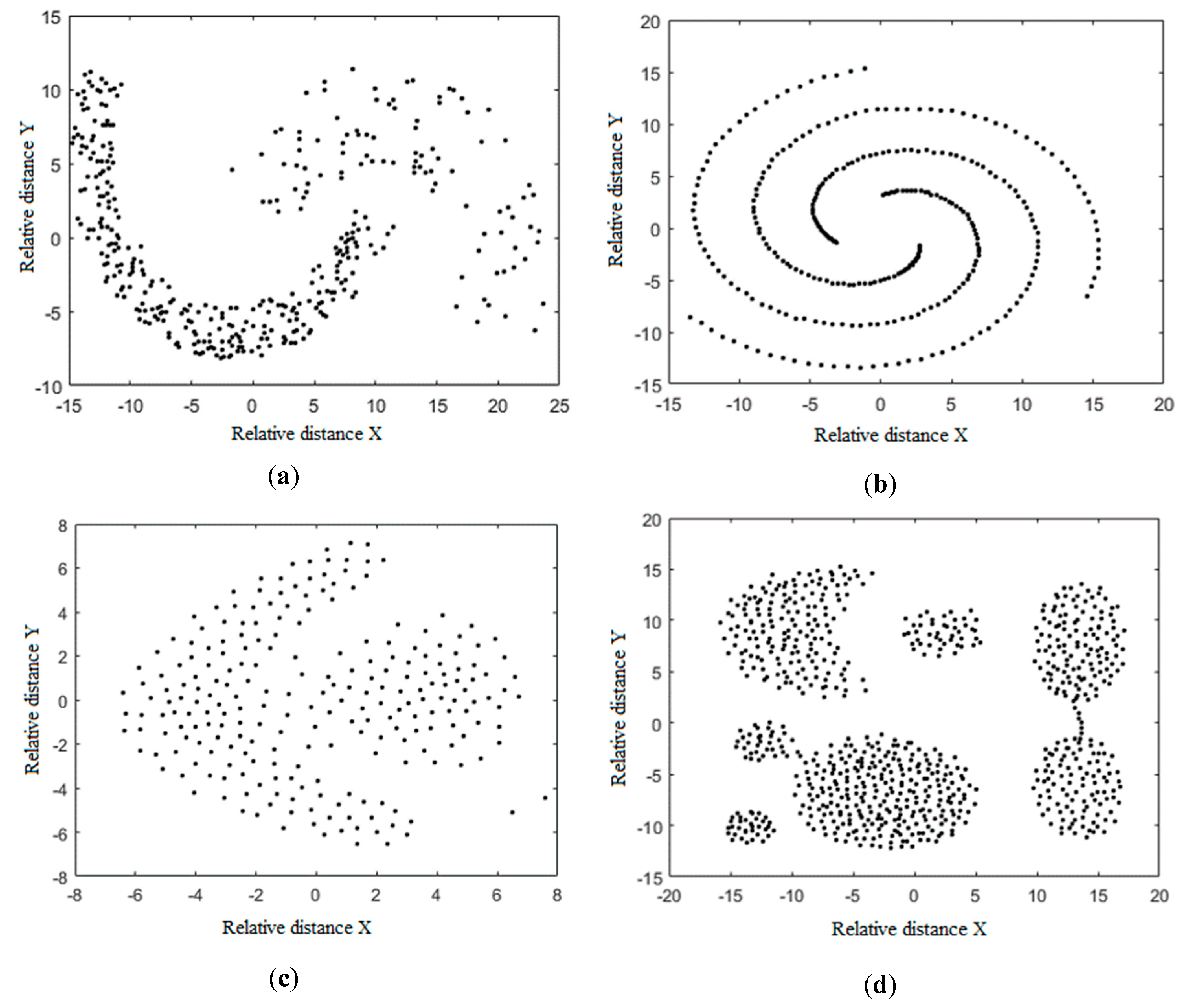
 [Green Version]
Figure 1. We first set the distance threshold to get the graph 1, (a) then input the topology into DeepWalk network 1. (b) The topological characteristics of each point of the data are obtained (c), which show the one-dimensional characteristics of 312 points. Then, the feature meaning correspondence is combined with the original data, and the topological feature is used as the weight to cluster the data to get 1. (d).
Electronics 09 00459 g001
Figure 2. In the decision graph, each point in the graph represents every point in the data set. It is not difficult to see from the graph that points with larger ρ i and δ i are more suitable to be cluster center points, and points with smaller ρ i value and larger δ i value are classified as outliers.
Electronics 09 00459 g002
Figure 3. (a) Shows the layout of the karate club data. (b) Shows the distribution of the two potential dimensions output by DeepWalk in the coordinate system. The horizontal and vertical coordinates represent the eigenvalues of DeepWalk with an output of two dimensions.
Electronics 09 00459 g003
Figure 4. After the topological transformation of the rectangle, point X is still in the rectangle. This built-in property becomes a topological feature.
Electronics 09 00459 g004
Figure 5. Density Peak Clustering Algorithm Considering Topological Features (DPCTF) algorithm flowchart. The first step of the algorithm is the rough arrow flow. The thin arrow is the second step of the process, combining the original data with topological characteristics, and finally clustering results are obtained by Clustering by Fast Search and Find of Density Peaks (CFSFDP) algorithm.
Electronics 09 00459 g005
Figure 6. The original data set.
Electronics 09 00459 g006
Figure 7. (a) Jain data, which has two classes, one of which is relatively dense and the other is relatively sparse, which is challenging to clustering problems to some extent; (b) spiral data, which is composed of three curve classes. K-means, DBSCAN and other clustering algorithms are not effective enough, and it will be challenging to verify our ideas. (c) Flame data set with evenly distributed data points to test the performance of clustering algorithm for non-discontinuous data sets; (d) aggregation data set, composed of seven classes, which tests the ability of the algorithm to deal with multi-categories. The above data sets basically cover the challenges of common clustering algorithms and verify our algorithm by their actual clustering effect.
Electronics 09 00459 g007
Figure 8. In the picture shown, X and Y represent relative distance. It can be seen from the comparison results that there is a big gap between the results of the comparison experiment formed by (a,b), and the clustering results of (c,d) at the two most marginal data points are different, while there is no difference between the results of the comparison experiment of (eh).
Electronics 09 00459 g008aElectronics 09 00459 g008b
Figure 9. The effects of different topological features on clustering results are presented.
Electronics 09 00459 g009
Figure 10. Two-dimensional clustering results obtained by DPCTF algorithm.
Electronics 09 00459 g010
Table 1. Introduction of test data sets.
NameSizeAttributesClasses
Jain37332
Spiral31233
Flame24032
Aggregation78837

