Modelling the Publishing Process of Big Location Data Using Deep Learning Prediction Methods

Abstract

Centralized publishing of big location data can provide accurate and timely information to assist in traffic management and for facilitating people to decide travel time and route, mitigate traffic congestion, and reduce unnecessary waste. However, the spatio-temporal correlation, non-linearity, randomness, and uncertainty of big location data make it impossible to decide an optimal data publishing instance through traditional methods. This paper, accordingly, proposes a publishing interval predicting method for centralized publication of big location data based on the promising paradigm of deep learning. First, the adaptive adjusted sampling method is designed to address the challenge of finding a reasonable release time via a prediction mechanism. Second, the Maximal Overlap Discrete Wavelet Transform (MODWT) is introduced for the decomposition of time series in order to separate different features of big location data. Finally, different deep learning models are selected to construct the entire framework according to various time-domain features. Experimental analysis suggests that the proposed prediction scheme is not only feasible, but also improves the prediction accuracy in contrast to the traditional deep learning mechanisms.

1. Introduction

Big location data refer to a dataset that encompasses location information and is large in scale, fast in production, and rich in value. Accurate and timely publishing of big location data is an indispensable constituent of modern Intelligent Transportation Systems (ITS), which assist in traffic management and facilitate users to plan travel time and route, mitigate traffic congestion, and reduce unnecessary waste [1,2]. Centralized publishing of big location data mainly provides statistical information pertinent to real-time traffic data. The publishing process has the typical time series characteristics. Taking into consideration the application requirements of ITS as an example, the big data publishing platform counts and releases the traffic flow within a certain area at regular intervals to help users keep abreast of traffic conditions, make personal travel plans, obtain location-based services, etc.

If we use $X_{t_i}$ to represent the location dataset corresponding to the publishing time $t_i$, then the dynamically released big location data can be expressed in the form of a time series as: $\left\{Y\left(t\right)\mid y\left(t\right)={\mathit{X}}_{{\mathit{t}}_1},{\mathit{X}}_{{\mathit{t}}_2},\dots ,{\mathit{X}}_{{\mathit{t}}_i},{\mathit{X}}_{{\mathit{t}}_{i+1}},\dots \right\}$. The real challenge is to ascertain an optimal data publishing instance that plays a critical role in ascertaining the utilities of published data. Traditional schemes employ a fixed time interval approach that implies averaging the published data from the aspect of the time dimension. Furthermore, determining the fixed time interval usually relies on the experience of experts that have poor reliability in practical applications. If the time interval is too large, the published dataset may miss the real maximum (i.e., upper) or minimum (i.e., lower) time period of traffic flow. This will seriously compromise the application performance of big location data. Users may not be able to schedule their travel at reasonable times or get stuck in traffic jams. On the contrary, if the time interval is too small, the amount of storage, operations, and calculations required for data publishing would increase sharply, thereby leading to an unnecessary waste of resources [3]. Therefore, the publishing process of big location data should be adaptively adjusted in order to reflect the dynamic changes in location data accurately and the availability of published data at the same time.

Big location data are random in nature, highly dynamic over time, and often affected by diverse factors, i.e., users, vehicles, roads, and environment. In addition to their features of being large in data volume, extremely rapid updates, and high monetary value, they also have the following special characteristics [4,5]:

• Temporal correlation: Although the total volume and update frequency of big location data change at a dynamic pace, the variation is not that huge for the adjacent data release within a certain time frame. This implies that observations at the adjacent time intervals are highly relevant. For example, a traffic congestion taking place during the morning peak hour, i.e., around 7:00 a.m, would probably last until 9:00 a.m.
• Spatial correlation: Combined with the distribution of urban roadside infrastructure and traffic networks, there is a certain spatial distribution pattern in the dense traffic areas of location big data. That is, the observations gained at nearby locations are correlated with each other, subsequently leading to local coherence in space.
• Periodicity: Peoples’ work and life follow a certain regularity, for instance both working days and off days have alternate patterns reflected in big location data. Through the visual analysis and long-term observation of the spatial and temporal distribution, it is easy to note that there is a clear similarity among the days and between the weeks.
• Heterogeneity: Heterogeneity means that the contribution of correlations to the final prediction results is not globally the same. Location data have a heterogeneous nature both in space and time. For instance, the peak hours and rapid changes are much more important than the off-peak hours for the purpose of ensuring accurate forecasting. Similarly, even within the same period of time, the densely populated commercial area is more important than the inaccessible far suburbs from the aspect of spatial characteristics.
• Randomness: Randomness primarily refers to the irregularity of location data in both time and space distribution. Although there are certain patterns in the time, place, and trajectory of peoples’ lives and work, we still cannot accurately predict when and where users would appear or even the exact number of people in the preceding second within a certain area.
• Uncertainty: Uncertainty mainly refers to the unpredictability of location data. For example, owing to weather changes, traffic events, and the behaviour of traffic participants, location data may suffer fluctuations and shift in the highest and lowest values in contrast to normal ones.

The spatial and temporal correlation and periodic characteristics make it possible to predict the amount of traffic flow, whereas the randomness and uncertainty bring great difficulties to the predictive work. According to the sampling theorem [6], the issue of predicting the publishing time can be transformed into a forecasting problem for publishing interval series. Generally, there are two major types of prediction methods for time series data [7,8], i.e., model-driven approaches and data-driven approaches. The former usually requires a good understanding of the model against the predicted object and is predetermined based on strong theoretical assumptions so as to establish an accurate mathematical expression model for the researched object. However, the randomness and uncertainty of big location data make it difficult to find a suitable model for accurate description within the existing mathematical domain. Therefore, such methods are difficult to develop and apply in practice. A data-driven prediction method is performed in the case of a black box. It is based on the collection of historical data, whereby the relevant hidden information can be mined through data analysis and processing methods and the original model is used to fit the data to make predictions. This method overcomes the shortcomings of model-driven prediction methods and adapts rapidly in practical applications. As a typical representative of data-driven methods, deep learning can automatically extract valuable information from a large number of complex unstructured data, such as features, categories, structures, and probability distributions. This also facilitates deep learning and big data applications to have natural matching characteristics, in turn making them suitable for the analysis and mining of nonlinear data models in big data environments [9].

In this paper, we propose a publishing interval predicting method for big location data based on deep learning models. The main contributions of our paper are as follows:

• We propose an adaptive adjusted sampling method to convert the problem of finding an optimal release time of big location data into a prediction problem for ascertaining the release time interval. This sampling and transformation method makes it possible to use deep learning methods in the later stage.
• We introduce the Maximal Overlap Discrete Wavelet Transform (MODWT) [10] method into the decomposition process of the location data sampling interval, which has proven to be helpful in describing sub-sequences with different characteristics and for enhancing the time series prediction accuracy.
• By analysing the characteristics of big location data, we select the main trends and fluctuations to be the two major features and accordingly adopt appropriate deep learning models to propose a release interval prediction method. Experimental results demonstrate that the prediction results of the proposed method improve to a significant degree as compared to the traditional models.

The rest of the paper is organized as follows. Section 2 outlines the existing state-of-the-art in the area of traffic prediction using deep learning models. Section 3 introduces the sampling and transformation method of historical big location data. Section 4 provides the basic principle and implementation method of MODWT decomposition. Section 5 explains the system model of the prediction method based on deep learning. Section 6 reports a set of empirical studies and the simulation results, and Section 7 concludes the paper.

2. Literature Review

Over the past few years, a varying number of methods has been proposed to enhance the accuracy of time series forecasting. Among them, the most correlated work with this paper is the prediction of traffic flow. Arief et al. investigated the correlation between weather parameters and traffic flow and proposed a novel holistic architecture to enhance prediction accuracy by incorporating a Deep Belief Networks (DBN) and weather prediction and decision-level data fusion scheme [11]. Yang et al. proposed a stacked autoencoder Levenberg–Marquardt model to improve forecasting accuracy [12]. The proposed model used the Taguchi method to develop an optimized structure and to learn traffic flow features through layer-by-layer feature granulation with a greedy layer-wise unsupervised learning algorithm. Zhao et al. proposed a novel traffic forecast model based on an LSTM network, which considered temporal-spatial correlation in a traffic system via a two-dimensional network composed of many memory units [13]. Chen et al. established a fuzzy deep convolutional network to improve traffic flow prediction [14]. This approach was built on fuzzy theory and the deep residual network model, and the key idea was to introduce the fuzzy representation into the DL model to lessen the impact of data uncertainty. Qu et al. presented a traffic prediction method using a deep neural network based on historical traffic flow data and contextual factor data [15]. The main idea was that traffic flow within a short time period was strongly correlated with the starting and ending time points of the period together with a number of other contextual factors, such as days of week, weather, and season. Therefore, the relationship between the traffic flow values within a given time interval and a combination of contextual factors could be mined from historical data. Zhang et al. employed the residual neural network framework to model the temporal closeness, period, and trend properties of crowd traffic. Residual convolutional units were designed for each property to model the spatial properties of crowd traffic. The proposed ST-ResNet approach outperformed many well-known methods [16]. Ren et al. proposed a deep spatio-temporal residual neural network for road network-based data modelling [17]. The proposed DSTR-RNet model constructed locally-connected neural network layers (LCNR) to model road network topology and integrated residual learning to model the spatio-temporal dependency, which maintained the spatial precision and topology of the road network, as well as improved the prediction accuracy. Wu et al. proposed a DNN-Based Traffic Flow prediction model (DNN-BTF) to improve the prediction accuracy, which made full use of the weekly/daily periodicity and spatial-temporal characteristics of traffic flow [18]. An attention-based model was introduced into their work that automatically learned to determine the importance of past traffic flow. The convolutional neural network was used to mine the spatial features, and the recurrent neural network was used to mine the temporal features of traffic flow. Li et al. suggested to model the traffic flow as a diffusion process on a directed graph and introduced a Diffusion Convolutional Recurrent Neural Network (DCRNN) for traffic forecasting [19]. The proposed method captured the spatial dependency using bidirectional random walks on the graph and the temporal dependency using the encoder-decoder architecture with scheduled sampling. Guo et al. used 3D convolutions to capture the correlations of traffic data in both spatial and temporal dimensions automatically [20]. The proposed ST-3DNet approach had a novel recalibration block that could explicitly quantify the difference of the contributions of the correlations in space. The 3D convolutions and recalibration block were employed respectively to model the local patterns and long-term patterns and then aggregated together in a weighted way for the final prediction. To sum up, short-term traffic flow prediction based on deep learning has been extensively studied in the research literature in terms of generic models and prediction accuracy. However, to the best of our knowledge, there is no research study focusing on modelling the publishing process of big location data by employing deep learning prediction methods.

Time series decomposition can be used to separate time series into sub-sequences with varying characteristics for target analysis and data mining so that the local features of time series could be efficaciously studied in more depth [21]. A brief glimpse of the literature revealed that some researchers decomposed the original time series by the Empirical Mode Decomposition (EMD [22]) and Ensemble Empirical Mode Decomposition (EEMD [23]) methods, constructed deep learning prediction models for different parts of decomposition separately, and finally integrated the results of multiple prediction models to obtain the prediction results. This greatly reduced the impact of data fluctuations on the prediction performance. During the decomposition process of EMD/EEMD, the original time series of different distribution characteristics may be decomposed into different numbers of intrinsic mode functions (IMFs). The large number of IMFs may lead to a big cumulative error in the final result, consequently reducing the accuracy of the prediction model. MODWT is a linear filtering operation that can transform time series into a set of time-dependent wavelet and scaling coefficients [10]. Different from the Discrete Wavelet Transform (DWT), MODWT is a highly redundant, non-orthogonal transform, which retains downsampled values at each level of the decomposition. The redundancy of MODWT facilitates alignment of the decomposed wavelet and scaling coefficients at each level with the original time series, which enables a ready comparison between the time series and its decomposition. Ghosh et al. used MODWT to decompose the time series of the individual exchange rates and applied the random forest and bagging method on the decomposed components to model the prediction [24]. He et al. combined the MODWT method and mixed wavelet neural network (WNN) architecture to develop a WNN-M prediction model through a data-driven approach [25]. Prasad et al. used MODWT to resolve the frequencies contained in predictor data while constructing a wavelet-hybrid model for the forecasting of streamflow [26].

3. Sampling and Transformation Method

Location big data are collected in real time and are constantly updated and changed. Generally speaking, location big data are a continuous stream of data that changes over time and is characterized by uncertainty and unpredictability. In order to publish and use data of this nature, the location data that continuously originate from the data provider can be accumulated and released according to a certain frequency. This process reflects the dynamic nature of location big data in terms of achieving a certain balance between accumulating big data and publishing them at an optimal time interval with an appropriate publishing frequency.

Furthermore, the publishing frequency of location big data (or the publishing time interval between adjacent data snapshots) directly affects the effectiveness of the published data. Traditional methods use a fixed publishing time interval. Let $\mathit{P}$ be the sampling period; the published location big data can be represented as $\left\{\mathit{Y}\left(\mathit{t}\right)\mid \mathit{y}\left(\mathit{t}\right)=X\left(t+iP\right)\right\}$, where $i=0,1,2,\dots$. Although, this way, the overall trend of the original data is maintained, nevertheless, the effect of published data is far from satisfying the users’ needs for real-time application of location big data. In particular, if the time interval T is set to be large, the published location big data snapshot is likely to lose its peak and its frequent lowest points of the data change or result in a time shift of the overall trend. This seriously impacts location-based service, e.g., users would not be able to schedule their respective travels at reasonable times. If the publishing time interval T is set too small, the computational overhead, analysis, privacy protection, etc., on the location big data snapshot would increase sharply, resulting in the unnecessary waste of precious resources.

If the dynamically changed location big data are released according to the data snapshot mode, the number of location points aggregated in two non-overlapped time segments are expressed as mutually independent random variables. If the probability distribution of the number of location points aggregated in $\left[\mathit{t},t+\tau \right]$ is approximately $P\left[Y\left(t+\tau \right)-Y\left(t\right)=k\right]=\frac{e^{-\lambda \tau }{\left(\lambda \tau \right)}^k}{k!}$, where $k=0,1,2,\dots ,n$ and $\lambda$ is a positive number (also referred to as the arrival rate), then the publishing process of location big data can be considered as a Poisson process with parameter $\lambda \tau$ [27]. Furthermore, if the publishing time of the first data snapshot is $t_1$ and $t_n$ represents the time interval between the (n − 1)th data snapshot and the nth data snapshot, then the publishing process of location big data can be expressed as a Poisson sample with the expected value of $\frac{1}{\lambda }$. However, as highlighted earlier, the time series model reflecting the real changing process of location big data is a complicated chore and cannot be accurately expressed by some existing mathematical function models. Therefore, the only way is to construct some other functions, which are more aligned and synched with the features and characteristics of location big data.

In order to reflect the details of dynamic changes in location big data in an accurate manner, we design a more flexible adaptive sampling method in this section. Intuitively, when the frequency of location information update is high, the release time interval should be reduced or the release frequency should be increased to illustrate the changes in location big data fully. On the contrary, when the frequency of location information update is low, the release time interval between data snapshots should be increased or the release frequency should be reduced to save the amount of computational time spent on the privacy protection data publishing algorithm.

Definition 1.

(Changing rate). Let $Y\left(t_i\right)$ and $Y\left(t_j\right)$ represent the statistical values of two adjacent location big data snapshots. Then, the changing rate could be expressed as:

$$C{R}_j=\frac{Y\left(t_j\right)-Y\left(t_i\right)}{t_j-t_i}$$

(1)

Definition 2.

(Growth rate). The ratio of the changing rate to the statistical value of the location big data snapshot is referred to as the growth rate:

$$G{R}_j=\frac{C{R}_j}{Y\left(t_i\right)}$$

(2)

Definition 3.

(Adaptive sampling interval). The subsequent sampling time interval can be adaptively adjusted according to the degree of change in the growth rate of the previous sampling and is directly proportional to the previous sampling interval and the amount of data between the adjacent sampling. The adjustment strategy for the sampling interval is ascertained as:

$${\mathit{ASI}}_{j+1}=\left\{\begin{array}{cc}{\mathit{ASI}}_j+\alpha ·T\hfill & if G{R}_{\mathrm{j}}=0\hfill \\ {\mathit{ASI}}_j\hfill & if 0<\left|G{R}_{\mathrm{j}}\right|\le \theta \hfill \\ {\mathit{ASI}}_j-\beta ·T\hfill & if \theta <\left|G{R}_{\mathrm{j}}\right|\hfill \end{array}\right.$$

(3)

where α and β are positive adjustment coefficients. The larger the adjustment coefficient is, the greater is the increase or decrease on the sampling interval after adjustment. $T$ represents the adjustment range, which has a positive value greater than zero. Similarly, the larger the value of $T$, the greater the amplitude of each adjustment. θ is the threshold of the growth rate. The larger the absolute value of the growth ratio, the greater is the change in the amount of location data. At this time, it is necessary to reduce the sampling interval to track the change process of statistical data quickly. On the contrary, when the absolute value of the growth ratio is closer to zero, a smaller change occurs between different adjacent data snapshots. At this time, the previous sampling interval can be maintained or even increased in order to save more system resources.

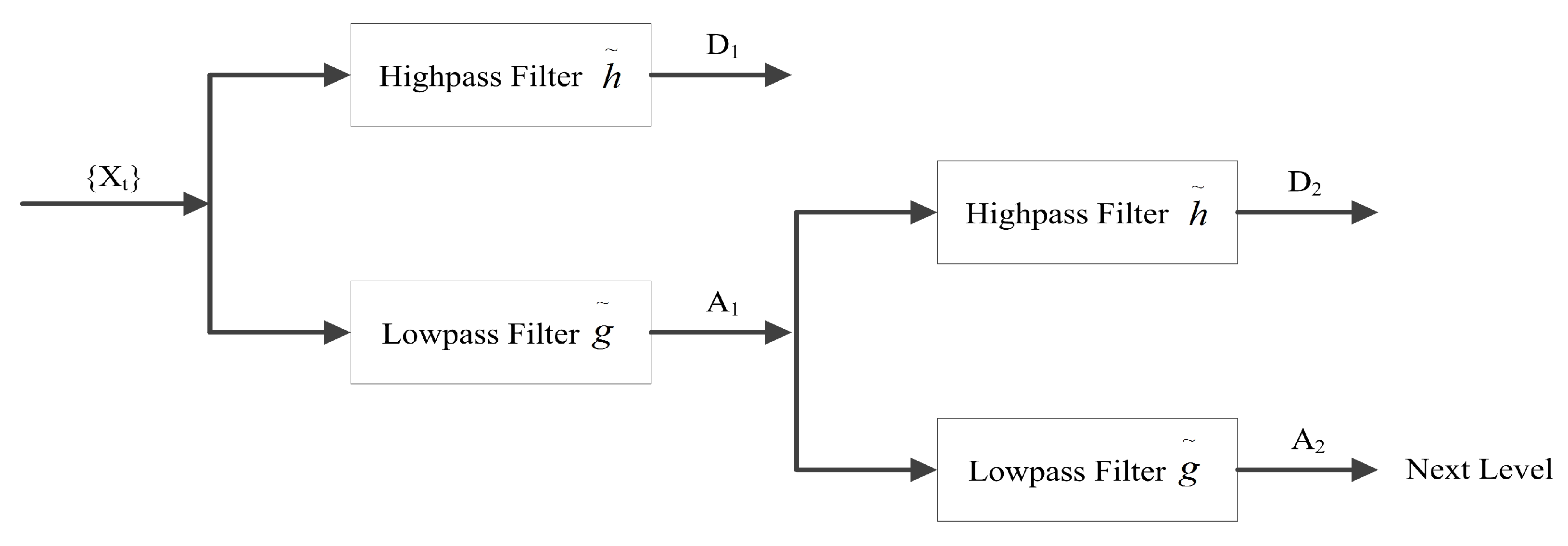
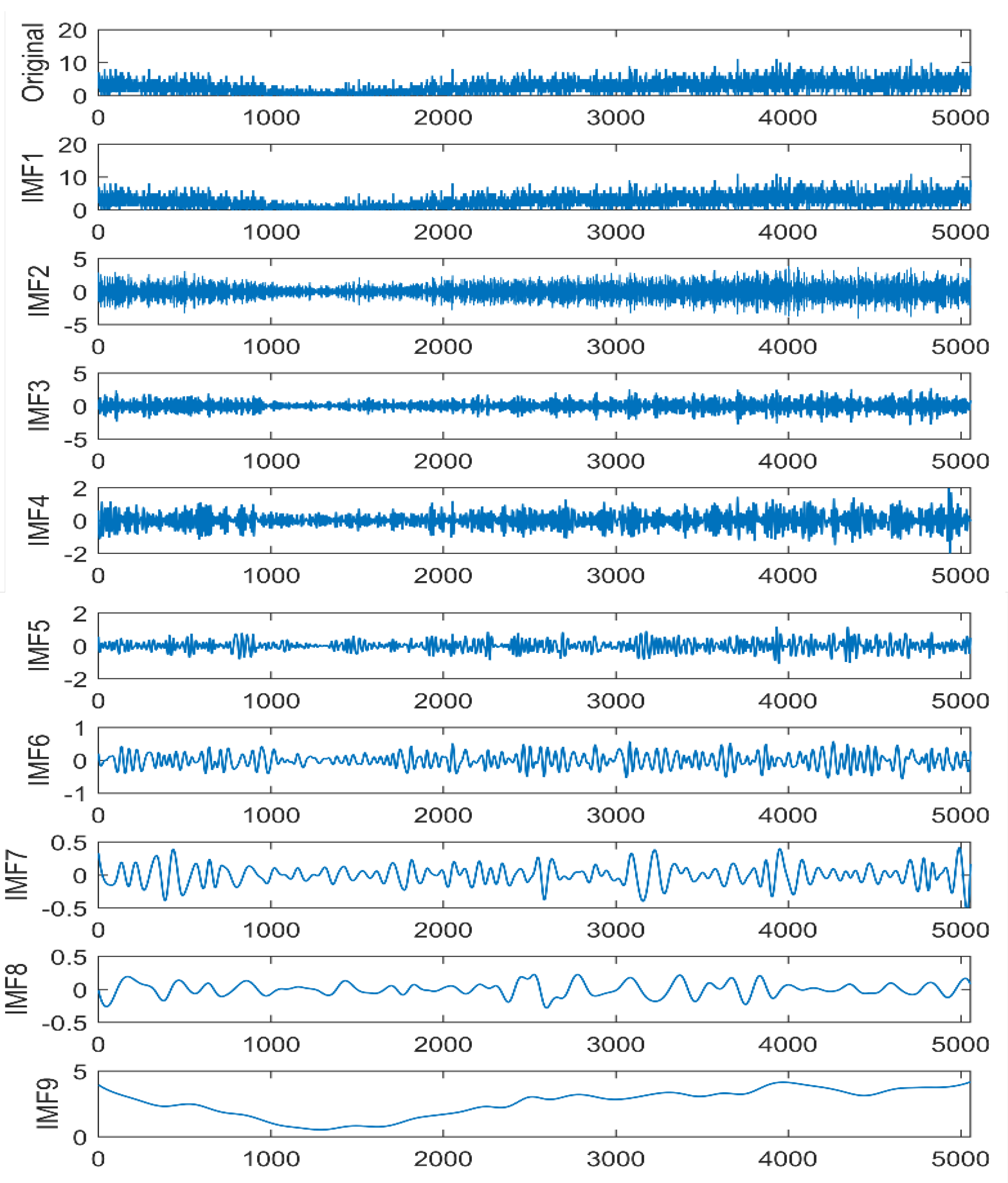
4. Time Series Decomposition

Due to the random changes in traffic demand, actual road conditions, and various external factors, the location big data present more complex fluctuation characteristics. This kind of volatility includes both linear persistence and nonlinear abruptness [5]. The former refers to the distribution characteristics of the current snapshot, and the release time would continue to affect the future snapshots and release time, thereby reflecting the medium- and long-term stable time-varying characteristics of big location data [9]. The latter refers to the leaping variation characteristics of location big data under the influence of external factors reflecting the random uncertainty of location big data, i.e., the abnormal changes caused by traffic flow changes, traffic events, weather conditions, and other random disturbances [4].

In this paper, we use MODWT [10] to decompose adaptively the sampling time interval sequence of big location data into the overall trend and its corresponding fluctuation characteristics. This helps to avoid the accumulation of errors caused by excessive decomposition and the subjective defects of artificially set parameters.

The principle of MODWT decomposition is shown in Figure 1. The result of r layer MODWT decomposition is comprised of the low frequency information (approximate part) of the rth layer and the high frequency information (details part) from the first layer to the rth layer. The MODWT of level $j_0$ has $\left(j_0+1\right)N$ coefficients, where N is the length of the signal in the sample.

The scaling filter ${\tilde{h}}_l$ and the wavelet filter ${\tilde{g}}_l$ of the MODWT transform are equivalent to the DWT filters as expressed in Equations (4) and (5):

$${\tilde{h}}_l=\frac{h_l}{\sqrt{2}}$$

(4)

$${\tilde{g}}_l=\frac{g_l}{\sqrt{2}}$$

(5)

For a finite input time series, $\left\{X_t\right\},t=0,1,\dots ,N-1$, the MODWT wavelet coefficients and scaling coefficients of the nth element in the first stage can be represented via Equations (6) and (7):

$${\tilde{W}}_{1,n}=\sum _{l=0}^{L_1-1}{\tilde{h}}_l{X}_{n-lmodN}$$

(6)

$${\tilde{V}}_{1,n}=\sum _{l=0}^{L_1-1}{\tilde{g}}_l{X}_{n-lmodN}$$

(7)

where L is the width of the filter.

Approximations and details of the first stage can be further calculated from Equations (8) and (9):

$${\tilde{A}}_{1,n}=\sum _{l=0}^{L_1-1}\widetilde{g_l}{\tilde{V}}_{1,n+lmodN}$$

(8)

$${\tilde{D}}_{1,n}=\sum _{l=0}^{L_1-1}\widetilde{g_l}{\tilde{W}}_{1,n+lmodN}$$

(9)

Similarly, the wavelet coefficient $\widetilde{W_j}$ and scaling coefficient $\widetilde{V_j}$ of the nth element on the jth stage can be ascertained from Equations (10) and (11):

$${\tilde{W}}_{j,n}=\sum _{l=0}^{L_j-1}{\tilde{h}}_{j,1}{\tilde{X}}_{n-lmodN}$$

(10)

$${\tilde{V}}_{j,n}=\sum _{l=0}^{L_j-1}{\tilde{g}}_{j,1}{\tilde{X}}_{n-lmodN}$$

(11)

Therefore, the approximations ${\tilde{A}}_j$ and the details ${\tilde{D}}_j$ of the nth element on the jth stage of the MODWT transform could be expressed as Equations (12) and (13):

$${\tilde{A}}_{j,n}=\sum _{l=0}^{L_1-1}{\tilde{g}}_{j,l}^0{\tilde{V}}_{1,n+lmodN}$$

(12)

$${\tilde{D}}_{j,n}=\sum _{l=0}^{L_1-1}{\tilde{h}}_{j,l}^0{\tilde{W}}_{1,n+lmodN}$$

(13)

If we want to get the value of the original data series, we only need the approximation of the jth layer and the details of each layer as shown in Equation (14):

$$X\left(n\right)=\sum _{l=0}^j{\tilde{D}}_j+{\tilde{A}}_j$$

(14)

With the help of the MODWT transform, the prediction problem of the non-stationary sequence can be converted into the prediction of the approximated and detailed parts after decomposition. Among them, the approximate part expresses the globalized trend of the original data sequence, and the detailed part reflects the local fluctuation characteristics. Corresponding deep learning models can be selected to predict the two parts separately, and the final result is integrated by MODWT reconstruction. The overall process is shown in Figure 2.

5. Predicting Publishing Interval Using Deep Learning Models

The randomness, non-linearity, and spatio-temporal correlation of big location data inhibit the traditional prediction mechanism to obtain the essential characteristics effectively. The deep learning method is inspired by the processing mechanism of the human nervous system. It uses computers to simulate human cognitive learning processes, build complex deep neural network structures through large-scale network neurons, and train the deep neural networks with large amounts of external data [28]. This is very helpful to extract the features of data automatically in a large amount of complex unstructured information and facilitates finding valuable information such as features, categories, structures, and probability distributions. The powerful non-linear function representation and feature extraction capability of deep learning help in overcoming the shortcomings of traditional prediction methods.

The publishing process of big location data conforms to typical time series characteristics. Therefore, the deep learning model can be set up to predict the reasonable release time and to optimize and adjust the publishing process dynamically. Centralized big location data publishing have typical periodic similarity and temporal correlation in the context of a statistical distribution. Periodic similarity mainly refers to the repeated appearance of certain regularities in the time dimension during the dynamic changing process of big location data. It is manifested as the inherent self-similarity and regularity of location big data. Through visual statistical analysis and long-term observation, we may find that the total amount of location information has clear similarities between days and among weeks depicting the obvious law of changes on working days and non-working days. Figure 3 shows the statistical information of taxi usage in New York City from 4–17 January 2009. Obviously, on the respective working days and non-working days, the trend waveform and total amplitude of the taxi usage maintained a high similarity, and the same results were also evident for a longer time range.

In our real lives, our travel time is affected by our living habits and travel modes, and so, there is a certain time pattern for the peak period of location information. During the adjacent release time, the amount of data change is within a certain range. As illustrated in Figure 3, the curve pertinent to total volume changes continuously and fluctuates to a slight extent showing obvious double-peak characteristics (corresponding to morning and evening peaks of traffic, respectively) during the working days from Mondays to Fridays; while on Saturdays and Sundays, there is a stepwise increasing trend. The period of these peaks also coincides with the daily work and life of people.

Combined with the above analysis, it was observed that the centralized publishing of big location data had obvious periodicity, change of trend, and local range fluctuation. The periodicity and changing trend together constituted the main feature of location data, whereas the fluctuation reflected the random change in location data. Therefore, we proposed a deep learning framework to decompose these two factors, adopted different deep learning models for varying characteristics, and eventually integrated them with various predictions to obtain the final result (shown in Figure 4). In terms of selecting the deep learning models, we chose Long Short-Term Memory (LSTM) and Gated Recurrent Unit (GRU) to train and predict the main trend and fluctuation of big location data, respectively, in order to overcome the shortcomings of the poor prediction stability of a single model, as well as to improve the accuracy of the overall prediction result.

LSTM is an excellent variant model of the Recurrent Neural Network (RNN). It inherits most of the characteristics of the RNN model and solves the vanishing gradient problem by using a gating function rather than an activation function [29]. By doing so, the network can remember the small gradients, no matter how deep the network is or how long the input sequence is. The LSTM model is suitable to learn from experience and to predict time series where there are fairly long time lags of unknown size between important events. Therefore, we selected the LSTM model to extract the trend and periodicity of publishing time interval series. In contrast to LSTM, the GRU model [30] has a simplified structure and takes in fewer parameters, thereby making it relatively easy to train and with less overfitting problems. In the LSTM model, the cell state of the previous layer and the forgetting vector are multiplied to determine whether this information needs to be remembered or discarded, whereas in the GRU model, the cell state is removed and the hidden state used to transfer information. In view of the above, in this paper, the GRU model is selected and applied to the training and prediction of local fluctuation characteristics.

6. Experiments and Analysis

6.1. Experimental Dataset and Baseline Methods

In order to evaluate the performance of the proposed publishing interval predicting method, we used the taxi record dataset, Yellow-tripdata (2009–2013) (https://www1.nyc.gov/site/tlc/about/tlc-trip-record-data.page), to carry out our experiments. Yellow-tripdata is a set of city-wide taxi order records provided by the New York City Government’s Taxi Management Committee. The taxi trip records include fields capturing pick-up and drop-off dates/times, pick-up and drop-off locations, trip distances, itemized fares, fare types, payment modes, and driver-reported passenger counts. In order to reflect the travel patterns of people in New York city, we counted the total number of taxis used per second to form the big location dataset. The final experimental dataset is summarized in

Table 1. Schema of the experimental dataset.

No.	Attribute Name	Description
1	Year	Year of the data (in “yyyy” format)
2	Month	The numerical value of the month in “mm” format (ranges from 1 to 12)
3	Weekdays	Days of a week, e.g., Monday; the values are displayed in numerical format ranging from 1 to 7, where 6 represents Saturday and 7 represents Sunday
4	Day	Defines the day of a month in “dd” format (ranges from 1 to 31)
5	Hours	Clock hours in numbers (starting from 0 to 23)
6	Interval Value	Numerical value of sampling intervals obtained by the adaptive adjusted sampling method on the experimental dataset

, which includes six attributes related to the prediction target. We implemented the proposed publishing interval predicting method based on Keras (https://keras.io/), which employs TensorFlow (https://www.tensorflow.org/) as its backend engine.

In order to evaluate the prediction performance of our proposed method, we conducted simulations and compared the result with the following baseline methods:

• HA: The average value of historical records at each corresponding time interval was used for ascertaining the prediction result.
• ARIMA: The Autoregressive Integrated Moving Average model is a classical method for time series analysis [31].
• LSTM: Long Short-Term Memory model is a special kind of RNN, which consists of a cell, an input gate, an output gate, and a forget gate. We used a simple LSTM model in our experiment, which contained 32 hidden units.
• GRU: The Gated Recurrent Unit model is a variant of LSTM, which only consists of a reset gate and an update gate. In our experiment, the GRU model also contained 32 hidden units.
• CNN: We used the 1-dimensional Convolutional Neural Network [32] to carry out the prediction work on publishing time interval series, which contained 32 filters, one maxpooling layer (size = 2), and 50 hidden units.
• CNN-LSTM: The Convolutional LSTM model [33] combines the characteristics of both the CNN and LSTM models and is widely used for the prediction of short-term traffic flow. During the experiments, the parameter settings were the same as those of the separate CNN and LSTM.

Table 2. Elaboration of the neural network structures.

Model	Details
LSTM	Layer (type)	Output Shape	Param
	LSTM	(None,32)	4992
	Dense	(None,1)	33
	Total params: 5025
GRU	GRU	(None,32)	3744
	Dense	(None,1)	33
	Total params: 3777
CNN	Conv1D	(None,5,32)	96
	Maxpooling	(None,2,32)	0
	Flatten	(None,64)	0
	Dense	(None,50)	3250
	Dense	(None,1)	51
	Total params: 3397
CNN-LSTM	TimeDist	(None,None,2,32)	96
	TimeDist	(None,None,1,32)	0
	TimeDist	(None,None,32)	0
	LSTM	(None,32)	8320
	Dense	(None,1)	33
	Total params: 8449

gives the elaboration of the neural network structure. All of the models used “tanh” and “MSE” as the activation function and loss function.

6.2. Comparison and Analysis of the Results

6.2.1. Sampling and Transformation Effect

In this experiment, fixed-interval sampling, Poisson sampling, and the proposed adaptive adjusted sampling method were carried out on the experimental dataset to convert historical location big data into sampling sequences. Parameters, i.e., entropy, expectation, variance, covariance, and time-domain skewness, were selected as the measurement indexes to compare the sampling conversion results of different methods. The fixed-interval sampling method used a time interval of 18$s$; the Poisson sampling parameter ($\lambda$) was 18; whereas the initial interval of the adaptive adjusted sampling was the same as the fixed-interval sampling method. The adjustment coefficient ($\alpha$) was two, and the adjustment range ($T$) was 1$s$. The rate of change was divided into three sub-intervals, i.e., ${\theta }_1$ = 0.1, ${\theta }_2$ = 0.3, and, ${\theta }_3$ = 0.5, and the corresponding adjustment parameters were ${\beta }_1$ = 1, ${\beta }_2$ = 3, and, ${\beta }_3$ = 5.

Table 3. Measurement index.

Measurement		Original	Fixed Sampling	Poisson Sampling	Adaptive Sampling
Entropy	Value	2.9278	2.8998	2.9296	2.9287
	Distortion	-	0.0096	0.0006	0.0003
Time-domain skewness		-	0.0472	0.1821	0.0179
Expectation	Value	2.7854	2.7939	2.8008	2.7968
	Distortion	-	0.0031	0.0055	0.0041
Variance	Value	4.4019	3.8174	5.2299	4.2788
	Distortion	-	0.1328	0.1881	0.028
Covariance	Value	4.402	3.8175	5.2301	4.2797
	Distortion	-	0.1328	0.1881	0.0278

depicts the daily average values against each measurement index. For discrete sequences, $\left\{X_t\right\}$, where $t=0,1,\dots ,N-1$, the definitions of entropy, expectation, and variance are expressed in Equations (15)–(17):

$$H\left(x\right)=-\sum _{i=1}^{N-1}p\left(x_i\right)logp\left(x_i\right)$$

(15)

$$\overline{X}=\frac{{\displaystyle \sum _{i=1}^{N-1}}{X}_i}{N}$$

(16)

$$S^2=\frac{{\displaystyle \sum _{i=1}^{N-1}}{(X_i-\overline{X})}^2}{N-1}$$

(17)

The covariance between the original discrete sequence $\left\{X_t\right\}$ and the sampled sequence $\left\{S_i\right\}$ can be ascertained from Equation (18):

$$\mathit{Cov}(X,S)=\frac{{\displaystyle \sum _{i=1}^{M-1}}(X_i-\overline{X})(M_i-\overline{M})}{M-1}$$

(18)

where $M$ is the total number of sampling points.

Let $Y$ represent the expectation, variance, or covariance of the original sequence and $\widehat{Y}$ represent the same parametric values of the sampled sequence. Therefore, the distortion rate can be represented as Equation (19):

$$D=\frac{\left|Y-\widehat{Y}\right|}{Y}$$

(19)

Let us suppose the maximum or minimum values of the original sequence appear at time $t_i$ and the maximum or minimum values of the sampling sequence appear at time $t_j$, then the ratio of the time deviation of the maximum or minimum values to the overall time range can be defined in terms of a time-domain skewness as shown in Equation (20):

$$\mathsf{\Delta }t=\frac{\left|t_i-t_j\right|}{\sum t}$$

(20)

Figure 5 portrays a comparison of the daily average distribution of the original location data sequence via various sampling conversion sequences. By observing the results of Figure 5 and comparing various performance indicators as depicted in Table 3, it can be noticed that the proposed adaptive adjusted sampling method reflected the change process of the original location data sequence within the overall distribution. Besides, it outperformed all of the other sampling methods in a much more effective manner.

Entropy is a measurement of the uncertainty of a random variable and represents the expected value of the amount of information that occurs in a randomly distributed event. In this experiment, the users’ travel demand per second was typically a random variable. It was affected by various factors such as time, location, weather, etc. It may be noted that the value of entropy only depended on the distribution of the random variable. Therefore, it could better reflect the distribution of users’ daily travel needs. The proposed adaptive adjusted sampling method obtained a much closer entropy value to the original time series, implying that it retained the distribution details of the original sequence in a better manner. Time-domain skewness indicates the ratio of the time deviation between the sampling sequence and the peak value of the original sequence to the overall time range. The proposed adaptive adjusted sampling method obtained the lowest skewness in the time domain, which manifested that it could reflect the change of big location data more dynamically. Expectation is an indicator to reflect the average value of random variables and depicts the relatively concentrated centre position of all the observations in the dataset. The sampling method with a fixed time interval had an average effect in the time domain. If the sampling time interval was small enough, the expectation value of the fixed time interval method was fairly close to that of the original sequence. However, this advantage will sharply decrease with the increase in the sampling time interval. Variance could be used to measure the degree of deviation between a random variable and its mathematical expectations. Covariance expresses the overall error of the said two variables. As is evident from Table 2, it can be found that the adaptive adjusted sampling method had the lowest variance, covariance, and distortion rate, which indicated that the sampling results obtained by this method had the smallest deviation from the original sequence distribution.

6.2.2. Time Series Decomposition Effect

Figure 6, Figure 7 and Figure 8 depicts the decomposition effect of the EMD, EEMD, and MODWT methods, respectively. Among them, 11 components were obtained by EMD decomposition, and the similarity coefficients of each component and the original sequence were 0.6189, 0.3723, 0.2444, 0.1783, 0.1242, −0.0270, 0.1369, 0.0017, −0.1361, 0.2336, and −0.2378. EEMD decomposition yielded nine components, and the similarity coefficients of each component and the original sequence were 1.0, 0.6363, 0.4033, 0.2725, 0.2085, 0.1405, 0.0828, 0.0730, and 0.5548 in sequence. Similarly, MODWT decomposition of one layer only obtained the two approximate and detailed components. The similarity coefficients with the original sequence were 0.6651 and −0.1011 respectively.

The 1–3, 4–7, and 8–10 components of the EMD decomposition (Figure 6) possessed certain similarities, which proved that the decomposition method had a modal aliasing phenomenon, thereby affecting the accuracy of subsequent prediction results. The EEMD decomposition (Figure 7) alleviated modal aliasing to some extent by adding white noise to the original signal during the decomposition process; nevertheless, the similarity coefficient between the recovered sequence and the original sequence reconstructed by all components was 0.9624. There was also a certain impairment to the accuracy of subsequent prediction results. The approximate low-frequency part of the MODWT decomposition (Figure 8) reflected the overall trend and period of the original data. The high-frequency details after removing the period and trend reflected the volatility of the original data. The volatility was relatively stable as a whole and was almost evenly distributed at zero. The similarity coefficient between the recovered sequence and the original sequence reconstructed by each component was one, which proved that the method possessed good reversibility. After the component decomposition and independent prediction were completed, the original characteristics of the overall sequence could be reconstructed to the greatest extent, and the prediction could be maintained.

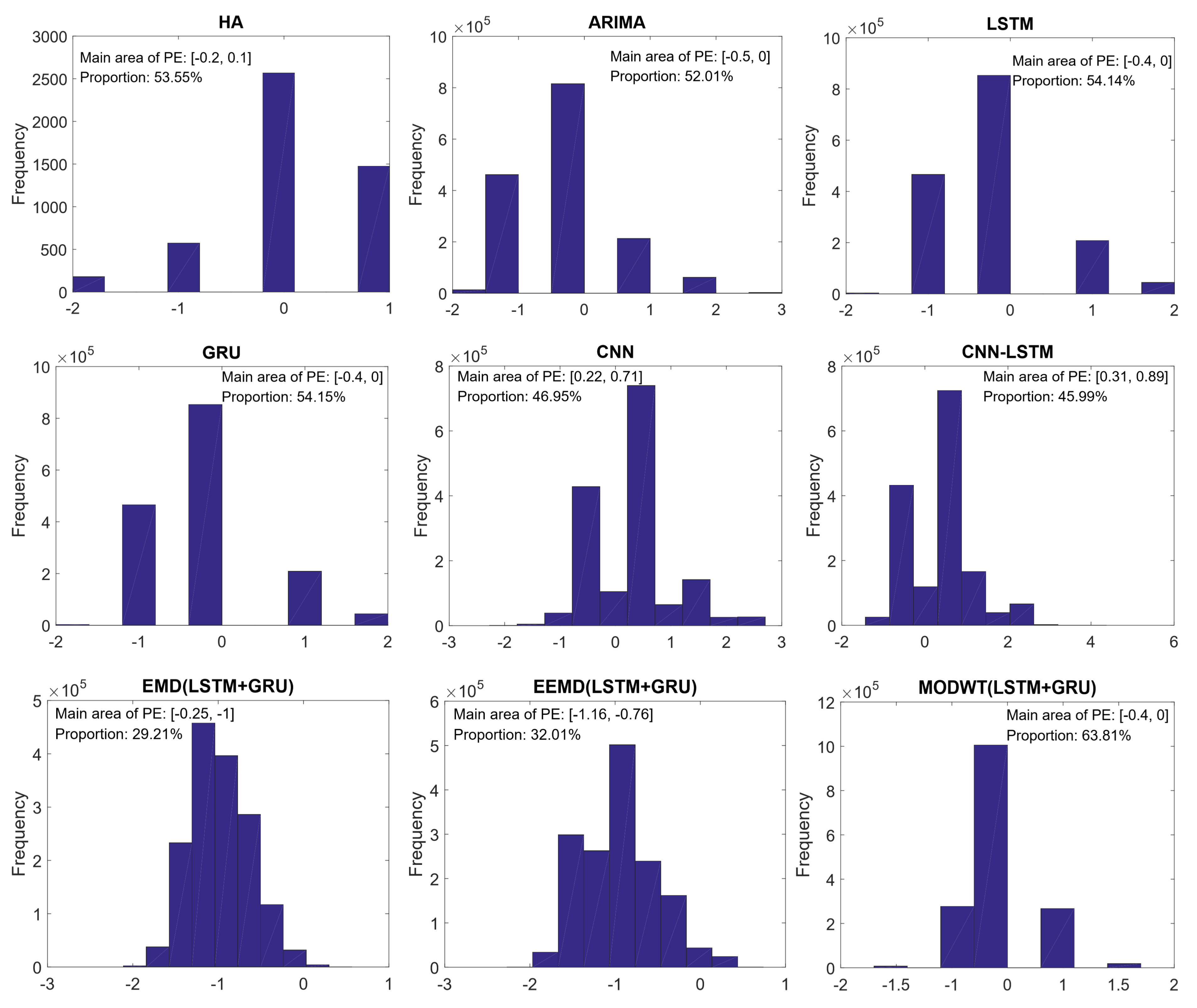
6.2.3. Prediction Effect

The prediction experiments were performed in the form of two groups. The first group used the baseline methods and historical data after adaptive adjusted sampling and divided the entire experimental dataset into training data and test data according to the ratio of 8:2. The other group first decomposed the time interval series after adaptive adjusted sampling and then used different deep learning models to predict different components separately and finally integrated the prediction results.

In

Table 4. Prediction performance of different methods.

Model	RMSE	MAE	MAPE
HA	0.7592	0.5018	2.952
ARIMA	0.6967	0.4745	2.8105
LSTM	0.6813	0.4642	2.7197
GRU	0.6806	0.4632	2.7143
CNN	0.7345	0.4851	2.879
CNN-LSTM	0.8435	0.544	3.2471
EMD (LSTM+GRU)	2.5042	1.8901	11.1532
EEMD (LSTM+GRU)	0.6747	0.4422	2.6282
MODWT (LSTM+GRU)	0.6003	0.3417	2.0301

, the EMD (LSTM+GRU) and EEMD (LSTM+GRU) methods used EMD and EEMD decomposition, respectively, and the LSTM and GRU models for prediction. For these two methods, the average value of the correlation coefficient of all components was employed as the threshold for dividing the main trend and the remainder. MODWT (LSTM+GRU) is our envisaged method, which uses one layer of MODWT decomposition to separate the main trend and the fluctuation. The prediction part uses the models and parameters similar to the above-mentioned methods. The final prediction result is obtained by inverse MODWT transformation.

In order to evaluate the performance of the proposed method, we used three performance metrics to evaluate the prediction result: Root Mean Squared Error (RMSE), Mean Absolute Error (MAE), and Mean Absolute Percentage Error (MAPE), which can be expressed via Equations (21)– (23):

$$\mathit{RMSE}=\sqrt{\frac{1}{n}\sum _{i=1}^N{\left(F_p-F_t\right)}^2}$$

(21)

$$\mathit{MAE}=\frac{1}{n}\sum _{i=1}^N\left|F_p-F_t\right|$$

(22)

$$\mathit{MAPE}=\frac{100}{n}\sum _{i=1}^N\left|\frac{F_p-F_t}{F_t}\right|$$

(23)

where $F_p$ represents the predicted value of the big data publishing interval and $F_t$ represents the true value of adaptive adjusted sampling.

The comparison results in Table 4 demonstrated that our method could achieve better prediction accuracy than the other baseline methods. It is pertinent to note that the HA method only obtained the result with a large amount of historical data. Furthermore, it did not analyse the spatial and temporal characteristics of location information. Therefore, its prediction accuracy was easily affected by different historical data samples. The ARIMA algorithm was suitable for prediction work based on a linear relationship, while on the contrary, the big location data were random and non-linear, and so, the prediction result was not optimal. Among the neural network algorithms, the LSTM and GRU models received better prediction accuracy and proved the feasibility of these two deep learning models in the prediction of big location data publishing. The CNN and CNN-LSTM models could process the spatio-temporal correlations and periodic features in the prediction work of short-term traffic flow. However, in our implementation, the final goal was only related to the time factor, and the prediction accuracy of the CNN model was slightly inferior to the above two models. In this respect, the combined use of CNN with LSTM dragged down the prediction accuracy of the original LSTM model. Among the decomposition-based prediction algorithms, the EMD (LSTM+GRU) method revealed the worst result. The problem of modal aliasing during EMD decomposition had a great impact on the prediction accuracy of the time series. The EEMD (LSTM+GRU) method achieved a better prediction accuracy than the other neural network algorithms with only one model. It proved that time series decomposition could indeed improve the accuracy of prediction. The proposed MODWT (LSTM+GRU) method obtained the lowest prediction error across all the performance metrics. The Root Mean Squared Error (RMSE) was enhanced by 11.89%, 11.80%, and 11.03% in contrast to the LSTM model, GRU model, and EEMD (LSTM+GRU) method, respectively. The Mean Absolute Error (MAE) of our method was 26.39%, 26.23%, and 22.73% higher than the LSTM model, GRU model, and EEMD (LSTM+GRU) method, respectively. The Mean Absolute Percentage Error (MAPE) of the proposed prediction method was also 25.36%, 25.21%, and 22.76% higher than the LSTM model, GRU model, and EEMD (LSTM+GRU) method, respectively. The results demonstrated the feasibility and effectiveness of the publishing interval prediction method based on deep learning. The adaptive adjusted sampling and MODWT decomposition method had a better effect on the pattern decomposition of big location data. The selected patterns and deep learning models had a good combination effect.

Figure 9 reflects the histograms of the frequency of Prediction Error (PE) via different methods. In order to better observe the distribution of prediction errors, we calculated the main distribution area of prediction errors and their proportion. Compared with the LSTM model and GRU model, the proposed MODWT (LSTM+GRU) method had the same domain and main area of PE. However, the proportion of the major distribution area of the MODWT (LSTM+GRU) method was much higher than the other two, which meant it had smaller error values. This was the reason that the proposed MODWT (LSTM+GRU) method achieved better prediction accuracy. On the contrary, the other decomposition and prediction methods, i.e., EMD (LSTM+GRU) and EEMD (LSTM+GRU), had a wider range of prediction error distributions and larger error values. Therefore, their prediction accuracy was not as good as the proposed MODWT (LSTM+GRU) method.

7. Discussion

The aforementioned analysis of the experiments proved the feasibility and efficaciousness of our envisaged interval prediction method based on deep learning for the centralized publishing process of big location data. By decomposing the release interval time series into sub-sequences of major trends and fluctuation characteristics via employing the MODWT method, separately predicting them, and finally, reconstructing the prediction result as a whole, the accuracy of prediction was considerably improved in contrast to other methods without sequence decomposition. This verified the role and advantage of the time series decomposition method in analysing and mining data features. Furthermore, the proposed MODWT (LSTM+GRU) prediction method combined the advantages of the LSTM model and GRU model in time series prediction. Furthermore, in contrast to the prediction methods using a single deep learning model, the prediction accuracy of the MODWT (LSTM+GRU) method was greatly improved. This was, therefore, a successful attempt to model the centralized publishing process of big location data using the deep learning methods that subsequently widened the application areas of deep learning technology. Furthermore, by decomposing the publishing data and selecting deep learning models according to different characteristics, it could be extended and applied to more application environments of big data publishing systems.

Nevertheless, this study focused only on the prediction of intervals for centralized publishing of big location data and was limited to our experimental datasets. In the near future, we intend to verify the proposed method via a real centralized big location data publishing system. Furthermore, some other additional information, i.e., such as weather conditions and traffic events, will be incorporated so as to improve the accuracy and meaningful prediction results for travellers, commuters, and administrative departments.

8. Conclusions

As one of the most active paradigms in the field of machine learning, deep learning has recently attained considerable attention in the fields of video tracking, image analysis, speech recognition, and text understanding. It can automatically extract original features in a large number of complex unstructured data and facilitates finding valuable information such as features, categories, structures, and probability distributions hidden in the data. However, to the best of our knowledge, as-of-date, there is no study in the existing literature focusing on the application of deep learning in big location data publishing systems. This paper, therefore, addressed the issue of modelling the centralized publishing process of big location data by employing deep learning methods. The adaptive adjusted sampling method converted historical location data into sampling interval series to predict a reasonable data publishing instance. In order to utilize the temporal correlation and periodicity features of big location data fully, the MODWT method was introduced into the decomposition process, which segregated the sampling series into the main trend and the fluctuation. The LSTM and GRU models were further adopted to perform the prediction of the above two components. Experimental analysis suggested that the proposed prediction method had better prediction accuracy in contrast to the traditional deep learning methods.

References

1. Ge, M.Z.; Bangui, H.; Buhnova, B. Big data for internet of things: A survey. Future Gener. Comput. Syst. 2018, 87, 601–614. [Google Scholar] [CrossRef]
2. Zhu, L.; Yu, F.R.; Wang, Y.; Ning, B.; Tang, T. Big Data Analytics in Intelligent Transportation Systems: A Survey. IEEE Trans. Intell. Transp. Syst. 2019, 20, 383–398. [Google Scholar] [CrossRef]
3. Yan, Y.; Zhang, L.X.; Sheng, Q.Z.; Wang, B.Q.; Gao, X.; Cong, Y.M. Dynamic release of location big data based on adaptive sampling and differential privacy. IEEE Access 2019, 7, 164962–164974. [Google Scholar] [CrossRef]
4. Pan, T.L.; Sumalee, A.; Zhong, R.X.; Indra-payoong, N. Short-Term Traffic State Prediction Based on Temporal–Spatial Correlation. IEEE Trans. Intell. Transp. Syst. 2013, 14, 1242–1254. [Google Scholar] [CrossRef]
5. Atluri, G.; Karpatne, A.; Kumar, V. Spatio-temporal data mining: A survey of problems and methods. ACM Comput. Surv. 2018, 51, 83. [Google Scholar] [CrossRef]
6. Zayed, A. Advances in Shannon’s Sampling Theory; Routledge: New York, NY, USA, 1993. [Google Scholar]
7. Weigend, A.S.; Gershenfeld, N.A. Time Series Prediction: Forecasting the Future and Understanding the Past; Taylor&Francis Group: Milton, UK, 2018. [Google Scholar]
8. Che, Z.; Purushotham, S.; Cho, K.; Sontag, D.; Liu, Y. Recurrent neural networks for multivariate time series with missing values. Sci. Rep. 2018, 8, 6085. [Google Scholar] [CrossRef] [PubMed] [Green Version]
9. Lv, Y.; Duan, Y.; Kang, W.; Li, Z.; Wang, F. Traffic flow prediction with big data: A deep learning approach. IEEE Trans. Intell. Transp. Syst. 2015, 16, 865–873. [Google Scholar] [CrossRef]
10. Percival, D.B.; Walden, A.T. Wavelet Methods for Time Series Analysis; Cambridge University Press: Cambridge, UK, 2000. [Google Scholar] [CrossRef]
11. Koesdwiady, A.; Soua, R.; Karray, F. Improving traffic flow prediction with weather information in connected cars: A deep learning approach. IEEE Trans. Veh. Technol. 2016, 65, 9508–9517. [Google Scholar] [CrossRef]
12. Yang, H.F.; Dillon, T.S.; Chen, Y.P.P. Optimized structure of the traffic flow forecasting model with a deep learning approach. IEEE Trans. Neural Netw. Learn. Syst. 2017, 28, 2371–2381. [Google Scholar] [CrossRef]
13. Zhao, Z.; Chen, W.; Wu, X.; Chen, P.C.Y.; Liu, J. LSTM network: A deep learning approach for short-term traffic forecast. IET Intell. Transp. Syst. 2017, 11, 68–75. [Google Scholar] [CrossRef] [Green Version]
14. Chen, W.; An, J.; Li, R.; Fu, L.; Xie, G.; Bhuiyan, M.Z.A.; Li, K. A novel fuzzy deep-learning approach to traffic flow prediction with uncertain spatial-temporal data features. Future Gener. Comput. Syst. 2018, 89, 78–88. [Google Scholar] [CrossRef]
15. Qu, L.; Li, W.; Li, W.; Ma, D.; Wang, Y. Daily long-term traffic flow forecasting based on a deep neural network. Expert Syst. Appl. 2019, 121, 304–312. [Google Scholar] [CrossRef]
16. Zhang, J.; Zheng, Y.; Qi, D. Deep spatio-temporal residual networks for citywide crowd flows prediction. In Proceedings of the 31st AAAI Conference on Artificial Intelligence, San Francisco, CA, USA, 4–9 February 2017; pp. 1655–1661. [Google Scholar]
17. Ren, Y.; Cheng, T.; Zhang, Y. Deep spatio-temporal residual neural networks for road-network-based data modelling. Int. J. Geogr. Inf. Sci. 2019, 33, 1894–1912. [Google Scholar] [CrossRef]
18. Wu, Y.; Tan, H.; Qin, L.; Ran, B.; Jiang, Z. A hybrid deep learning based traffic flow prediction method and its understanding. Transp. Res. Part C 2018, 90, 166–180. [Google Scholar] [CrossRef]
19. Li, Y.; Yu, R.; Shahabi, C.; Liu, Y. Diffusion convolutional recurrent neural network: Data-driven traffic forecasting. In Proceedings of the International Conference on Learning Representations, Toulon, France, 24–26 April 2017. [Google Scholar]
20. Guo, S.; Lin, Y.; Li, S.; Chen, Z.; Wan, H. Deep spatial-temporal 3D convolutional neural networks for traffic data forecasting. IEEE Trans. Intell. Transp. Syst. 2019, 20, 3913–3926. [Google Scholar] [CrossRef]
21. Huang, N.E.; Shen, Z.; Long, S.R.; Wu, M.C.; Shih, H.H.; Zheng, Q.; Yen, N.C.; Chao, T.; Liu, H. The empirical mode decomposition and the Hilbert spectrum for nonlinear and non-stationary time series analysis. Proc. R. Soc. Lond. 1998, 454, 903–995. [Google Scholar] [CrossRef]
22. Qiu, X.; Ren, Y.; Suganthan, P.N.; Amaratunga, G.A.J. Empirical mode decomposition based ensemble deep learning for load demand time series forecasting. Appl. Soft Comput. 2017, 54, 246–255. [Google Scholar] [CrossRef]
23. Wang, W.; Chau, K.; Xu, D.; Chen, X.Y. Improving forecasting accuracy of annual runoff time series using ARIMA based on EEMD decomposition. Water Resour. Manag. 2015, 29, 2655–2675. [Google Scholar] [CrossRef]
24. Ghosh, I.; Chaudhuri, T.D. Fractal Investigation and Maximal Overlap Discrete Wavelet Transformation (MODWT)-based Machine Learning Framework for Forecasting Exchange Rates. Stud. Microecon. 2017, 5, 105–131. [Google Scholar] [CrossRef]
25. He, F.; Zhang, Y.; Liu, D.; Dong, Y.; Liu, C.; Wu, C. Mixed Wavelet-Based Neural Network Model for Cyber Security Situation Prediction Using MODWT and Hurst Exponent Analysis. In Proceedings of the International Conference on Network and System Security, Helsinki, Finland, 21–23 August 2017; pp. 99–111. [Google Scholar]
26. Prasad, R.; Deo, R.C.; Li, Y.; Maraseni, T. Input selection and performance optimization of ANN-based streamflow forecasts in the drought-prone Murray Darling Basin region using IIS and MODWT algorithm. Atmos. Res. 2017, 97, 42–63. [Google Scholar] [CrossRef]
27. Menon, A.K.; Lee, Y. Predicting short-term public transport demand via in homogeneous poisson processes. In Proceedings of the 2017 ACM on Conference on Information and Knowledge Management, Singapore, 6–10 November 2017; pp. 2207–2210. [Google Scholar]
28. LeCun, Y.; Bengio, Y.; Hinton, G. Deep learning. Nature 2015, 521, 436–444. [Google Scholar] [CrossRef] [PubMed]
29. Hochreiter, S.; Schmidhuber, J. Long short-term memory. Neural Comput. 1997, 9, 1735–1780. [Google Scholar] [CrossRef] [PubMed]
30. Chung, J.; Gulcehre, C.; Cho, K.H.; Bengio, Y. Empirical evaluation of gated recurrent neural networks on sequence modelling. In Proceedings of the NIPS Deep Learning of Representations, Montreal, QC, Canada, 12 December 2014. [Google Scholar]
31. Ahmed, M.S.; Cook, A.R. Analysis of freeway traffic time-series data by using Box-Jenkins techniques. Transp. Res. Rec. J. Transp. Res. Board 1979, 722, 1–9. [Google Scholar]
32. Abdeljabera, O.; Avci, O.; Kiranyaz, S.; Gabbouj, M.; Inman, D.J. Real-time vibration-based structural damage detection using one-dimensional convolutional neural networks. J. Sound Vib. 2017, 388, 154–170. [Google Scholar] [CrossRef]
33. Xingjian, S.H.I.; Chen, Z.; Wang, H.; Yeung, D.Y.; Wong, W.K.; Woo, W.C. Convolutional LSTM network: A machine learning approach for precipitation nowcasting. In Proceedings of the Advances in Neural Information Processing Systems, Montreal, QC, Canada, 8–13 December 2015; pp. 802–810. [Google Scholar]
Figure 1. Process of MODWT decomposition.
Electronics 09 00420 g001
Figure 2. Process of MODWT reconstruction.
Electronics 09 00420 g002
Figure 3. Daily statistics of taxis on demand in New York City.
Electronics 09 00420 g003
Figure 4. A framework for predicting interval-based publishing of big location data based on deep learning. GRU, Gated Recurrent Unit.
Electronics 09 00420 g004
Figure 5. Comparison of different sampling methods.
Electronics 09 00420 g005
Figure 6. Decomposition effect of the EMD method.
Electronics 09 00420 g006
Figure 7. Decomposition effect of the EEMD method.
Electronics 09 00420 g007
Figure 8. Decomposition effect of the MODWT method.
Electronics 09 00420 g008
Figure 9. Histograms of the frequency of Prediction Error (PE) of different models.
Electronics 09 00420 g009