Improved KNN Algorithm for Fine-Grained Classification of Encrypted Network Flow

Abstract

The fine-grained classification of encrypted traffic is important for network security analysis. Malicious attacks are usually encrypted and simulated as normal application or content traffic. Supervised machine learning methods are widely used for traffic classification and show good performances. However, they need a large amount of labeled data to train a model, while labeled data is hard to obtain. Aiming at solving this problem, this paper proposes a method to train a model based on the K-nearest neighbor (KNN) algorithm, which only needs a small amount of data. Due to the fact that the importance of different traffic features varies, and traditional KNN does not highlight the importance of different features, this study introduces the concept of feature weight and proposes the weighted feature KNN (WKNN) algorithm. Furthermore, to obtain the optimal feature set and the corresponding feature weight set, a feature selection and feature weight self-adaptive algorithm for WKNN is proposed. In addition, a three-layer classification framework for encrypted network flows is established. Based on the improved KNN and the framework, this study finally presents a method for fine-grained classification of encrypted network flows, which can identify the encryption status, application type and content type of encrypted network flows with high accuracies of 99.3%, 92.4%, and 97.0%, respectively.

1. Introduction

Traffic-classification technology plays an important role in network security defense mechanisms. It is the basis for analyzing network traffic, detecting network anomalies, and balancing network load [1]. However, while traffic encryption is often used to protect information transmission, it also complicates the network traffic classification and analysis [2,3]. Nowadays, cyber attacks are usually implemented through encrypted traffic [4], and most of them are simulated as normal-application [5] or normal-content [6] network flows, which bypasses the network defense system and causes great damage. Thus, the fine-grained classification including the analysis of application and content types of encrypted traffic is an important research area [7].

Machine learning is a well-known method in the field of encrypted traffic classification [8]. But the machine-learning method needs a great amount of labeled data to train a model in terms of achieving fine-grained classification [9], and it is difficult to realize in an actual network for the reasons that labeled data are hard to obtain [10] and the model should be updated periodically for coping with concept drift [11,12].

Therefore, this study proposes a classification method using a model trained with a small amount of labeled data, which can achieve fine-grained and accurate classification of encrypted network flows. The K-nearest neighbor (KNN) algorithm is widely used to train an accurate model based on a small training set [13,14]. Traditional KNN determines the label of new data according to the labels of the K-nearest data points. The point distance calculation is based on non-weighted feature values, which is not appropriate enough to be implemented in the classification of network flows. For one thing, the influences of different traffic features are different to the actual distinction of two data points [15], i.e., the essential features accurately describe the distinction while useless features mislead the classification results. For another, the importance of a feature is different for different classification purposes. Thus, features selection and feature weights setting are key parts of fine-grained classification of traffic based on KNN.

This study aims to promote the performance of traffic classification by improving traditional KNN. Considering the different effects of different features, this study introduces the concept of feature weight and proposes a weighted feature KNN (WKNN) algorithm. To obtain the optimal feature set and the corresponding feature weight set, a feature selection and feature weight self-adaptive algorithm for WKNN (WKNN-Selfada) is proposed, which can be used to train a classification model for encrypted traffic identification. WKNN-Selfada can adjust weights according to each misleading sample, so it can fully learn the characteristics of the traffic just with a few training samples, which can meet the requirements of a small training set.

Furthermore, a framework for fine-grained classification of encrypted network flows is built, which analyzes three attributes of encrypted network flows, namely encryption status, encrypted application type, and encrypted content type. Fine-grained and multi-attribute classification is the basis of network management and network security analysis. Based on the framework, classification of network flows can be more meticulous, which provides many network analysis work with basic supports. For better understanding, we take a simple example. The framework can be used to analyze whether a flow is abnormal not only according to the single attribute value of a flow, but also the association between the attributes of the flow. For example, YouTube flow is normal flow in most cases and file flow is a normal flow in most cases, but a YouTube and file flow is likely a malicious flow, because the YouTube application usually produces streaming flows but hardly file flows. Thus, if we detect a flow as a YouTube flow as well as a file flow, the flow will be probably an anomaly. The framework we proposed can distinguish this type of abnormal flows based on the analysis of the correlation between the attributes.

Finally, based on the improved KNN algorithm and the framework, a new method for fine-grained classification of encrypted network flows (FCE-KNN) is proposed. This method implements the WKNN-Selfada algorithm to train classification models and uses these models for real-time traffic classification based on WKNN.

Th main contributions of this study are as follows:

(1) Aiming at solving the problem that different influences of features are not expressed accurately, improved versions of the traditional KNN algorithm are developed, namely the weighted feature KNN (WKNN) algorithm and the feature selection and feature weight self-adaptive algorithm for WKNN (WKNN-Selfada).

(2) To meet the requirement of network security analysis, a three-layer framework for fine-grained classification of an encrypted network flow is innovatively proposed, which can reinforce network security by analyzing the correlation of the fine-grained attributes.

(3) In order to realize accurate and fine-grained classification, a fine-grained classification of encrypted network flows based on the framework and the improved KNN algorithms (FCE-KNN) are presented, which can identify the encryption status, application type and content type of encrypted network flows.

The remainder of this paper is organized as follows. Section 2 reviews related studies on traffic classification. Section 3 introduces the notion of feature weight and proposes the WKNN and WKNN-Selfada algorithms. Section 4 discusses a fine-grained classification framework and proposes a corresponding fine-grained classification method for encrypted network flows. Section 5 presents the results of experiments on the public dataset Information Security Centre of Excellence (ISCX) VPN-nonVPN [16] (VPN: Virtual Private Network, one of the means of encrypting network traffic) to compare the performance of FCE-KNN with that of state-of-the-art algorithms. Finally, Section 6 summarizes the main findings of the paper.

2. Related Work

This study categorizes traffic-classification techniques from the perspective of extracted traffic features, as shown in Figure 1. The traffic-classification technology consists of static feature analysis and dynamic feature analysis. Static feature analysis mainly includes port detection and packet load detection, whereas dynamic feature analysis mainly includes statistical feature analysis and behavior analysis. Statistical feature analysis includes machine-learning methods and general statistical feature methods.

The port-detection technology implements traffic classification by detecting the port number of packets, but it is not always useful owing to the abuse of the non-standardized port number. Deep packet inspection (DPI) [17,18] and deep flow inspection (DFI) [19] implement analysis on packets or flows through frequent item-mining and pattern-matching methods, but it is difficult to establish matching rules for encrypted traffic. The behavior detection method [20,21,22,23,24] achieves high identification accuracy of encrypted traffic only for some special applications or protocols. The methods based on statistical features currently show relatively good performance for encrypted traffic classification, and machine learning (ML) is the most popular and effective one among them.

From the perspective of basic ML methods, decision trees [25,26] showed good performance in most cases, but over-fitting can easily occur, leading to poor classification in actual networks. Cluster methods [27,28] could achieve traffic classification without labeled data, but it was difficult to find a really useful and suitable clustering metrics. Bayesian methods [29,30] provided probability-based predictions, but their performance was poor when there were correlations between features, as was usually the case. Support vector machines (SVM) [31] had general adaptability to encrypted traffic classification, but the algorithm had high complexity and was very time consuming. Although ensemble learning [32,33] showed good performance, the model based on a weak learner lacked interpretability. Neural networks [34,35,36,37,38,39,40,41,42,43] needed a large amount of data to train a model, which was difficultly to realize in a condition of a small training set. Transfer learning [44] and active learning [45] addressed the issues of model practicability and insufficient label data during training, respectively, but they have not been adequately explored in studies on fine-grained classification. Various machine-learning methods had been combined to build hybrid models [46,47,48] in progressive or parallel structures [49], but most of the models were too complex for real-time classification. For the general statistical feature methods, Dorfinger et al. [50] identified encrypted traffic according to the entropy of packet data; however, some studies [1,29] have recently found that the entropy method cannot distinguish between encrypted traffic and compressed traffic. Among them, KNN [51,52,53] is light and accurate, and could train a high-performance model with a small amount of labeled data. But to some extent, the non-weight distance calculation lacks adaptability to different tasks of encrypted traffic classification. Carela-Español et al. [54] used KD-Tree (k-dimension tree) to improve the efficiency of KNN in traffic classification. Bar-Yanai et al. [55] combined KNN and K-means to improve the efficiency for real-time traffic classification. However, These two methods did not solve the problem of fine-grained classification.

From the perspective of methods including feature selection or feature weight training, McGaughey et al. [56] used the fast orthogonal search algorithm for traffic feature selection. Dong et al. [57] proposed a multi-objective adaptive feature selection algorithm for traffic classification based on information gain rate and evolutionary computing. Saber et al. [58] achieved traffic feature selection based on linear discriminant analysis. Manju et al. [59] ranked traffic features according to the feature weights which were the number of times that each feature appears in the tree, and selected the optimal feature subset based on the accuracies of the extreme gradient boosting model. Jamil et al. [60] created several candidate feature subsets by different feature selection algorithms, and chose the best subset according to the results of all the feature subsets’ evaluations based on the five ML algorithms. The feature weighted or feature selection method based on KNN [61] has been studied comprehensively in many areas, such as transportation system [62], anomaly detection [63,64], image identification [65] and so on, except for the fine-grained classification of network traffic. Only Dong et al. [66] in 2017 presented a modified version of consistency-based method in combination with a layered KNN classifier to evaluate the goodness of a feature subset.

3. Improvement of K-Nearest Neighbor (KNN) Algorithm

This section introduces the notion of feature weight, improves the distance calculation formula in KNN, and proposes the weighted feature KNN (WKNN). Furthermore, this section also includes our proposed feature selection and feature weight self-adaptive algorithm for WKNN (WKNN-Selfada), considering how to choose the appropriate feature set and the optimal feature weight set.

3.1. Weighted-Feature KNN

KNN is a supervised machine learning algorithm that finds a similarity between two points by calculating the distance between them. KNN first calculates the distances between each training sample and the target point, and then selects the k-nearest samples to the target point. These k samples jointly determine the class of the target point. The distance calculation of features is a direct means for expressing the similarity of points, and KNN shows excellent performance in predicting the target network flow.

Minkowski distance is one of the widely used distance metrics in traditional KNN, shown in below. If traffic features have no scale and have the same data distribution, Minkowski distance can express the actual distance between two points. In this paper, the exponent of the differences between the feature values is set to 2, which is Euclidean distance, because square sum is beneficial to describe the multi-dimension point distance. When the feature dimension of points is m, the formula for calculating the point distance between training sample $p={(x}_1{,\dots ,x}_m)$ and test point $q={(y}_1{,\dots ,y}_m)$ is given by distance $=\sqrt{{{\displaystyle \sum }}_{j=1}^m{{(x}_j-y_j)}^2}$. The shorter the distance between the two points, the greater is the similarity between them. After calculating the distances of all point pairs, the k-nearest training samples determine the class of the test point.

The distance calculation of traditional KNN is non-weighted, which means that it does not reflect the different effects of different features in traffic classification. This paper introduces feature weight and weighted feature-based point distance to improve the adaptation of the classification model to encrypted traffic-classification tasks. We use data normalization to eliminate the data scales for the implementation of Minkowski distance. Based on Euclidean distance, we make improvements on the traditional KNN, and several definitions are shown below.

Definition 1 (Feature weight).

is the coefficient of the feature when calculating the distance between two points. The weights of features are represented by a column vector,$w={(w}_1{;\dots ;w}_m)$, where m is the dimension of the features.

Feature weights reflect the importance of features during distance calculation. The larger the feature weight, the greater is the influence of the feature on the traffic classification.

Definition 2 (Feature distance).

is the square of the difference between two points’ feature of the dimension. For points$p={(x}_1{,\dots ,x}_m)$and$q={(y}_1{,\dots ,y}_m)$, the feature distances are calculated and represented by$fd={[(p-q).]}^2=((x_1-y_1{)}^2{,\dots ,(x}_m-y_m{)}^2)$, where${[(p-q).]}^2$means squaring each elements of the vector$(p-q)$. If there are several pairs of two points, the feature distances would be formed a matrix, represented by FD, and${fd}^{(i)}$means the ith pair’s feature distances.

Definition 3 (Weighted feature-based point distance).

is based on the Minkowski distance with the additional introduction of the feature weight. For points p, q and the feature weights w, the weighted feature-based point distance is given by distance$=\sqrt{fd·w}=\sqrt{{\left[\right(p-q).]}^2·w}$.

The weighted-feature KNN (WKNN) algorithm is proposed in this paper, shown in Algorithm 1. The inputs of the algorithm are the training sample set, a matrix P, target point q, parameter k, and feature weight w. The shape of the matrix P is (n, m), where n is the number of training points and m is the feature dimension, and $p^{\left(i\right)}$ means the ith row of P. The outputs are the class prediction result of the target point q, the weighted feature-based point distances between the k-nearest neighbors and q, kDistances, the matrix of feature distances between each k-nearest neighbor and q, KFD, and the classes of the k-nearest neighbors, kClass. Some of the outputs are used for Algorithm 2, which will be described later.

First, in lines 1–5, the algorithm calculates the feature distances between each training point $p^{\left(i\right)}$ and q, and then calculates the corresponding weighted feature-based point distance, where distances[i] means the ith pair’s weighted feature-based point distance and distances is an array.

Next, in lines 6–9, the algorithm calculates the information of the k-nearest neighbors. knnIndex is the corresponding indexes of the k-nearest neighbors. kDistances is the weighted feature-based point distances of the k-nearest neighbors. KFD is the feature distances matrix of the k-nearest neighbors. kClass is the labels of the k-nearest neighbors. argminK() is a function to get the indexes of the k smallest elements from small to large, and class() is to get the label of the point.

Finally, in lines 10–14, it calculates the prediction scores. WKNN uses the reciprocal of each k distance value as a weight to be added to the score of the corresponding class and output the class with the highest score as the prediction result.

Algorithm 1: WKNN

3.2. Feature Selection and Feature Weight Self-Adaptive Algorithm for Weighted Feature KNN (WKNN)

The selection of the feature set and the setting of the corresponding feature weights determine whether the calculated point distance can accurately represent the similarity between two points. To achieve more effective classification, a feature selection and feature weight self-adaptive algorithm for WKNN (WKNN-Selfada) is proposed, which can adapt feature weights by itself based on training data, instead of by manual setting. The algorithm learns the influence and updates the weights of features by analyzing only one sample at a time, so it can fully learn and adapt well to the law of each training sample and realize accurate classification just with a small training set.

The algorithm includes two parts, which runs two times and achieves a single part each time. The first time of the algorithm adapts the feature weight of each feature in the candidate feature set and selects the optimal feature set by comparing the weights with the feature selection threshold. In the second time of the algorithm, after feature selection in the first time, the weights of the selected features are retrained, because the new feature set is not the same with the original feature set and the weights of the original features cannot express the actual influences and mutual relation of the newly selected features. In the process of weight adjustment, the algorithm suggests that the feature with a larger feature distance would play a greater role in distinguishing the two points with different classes once misclassification. Therefore, when updating the weights, the weights of features with a large feature distance are supposed to increase while those with a small feature distance are supposed to decrease in order to increase the point distance between two points with different classes and reduce the possibility of misclassification. Thus, the accuracy of identifying the class of the test point can be improved further.

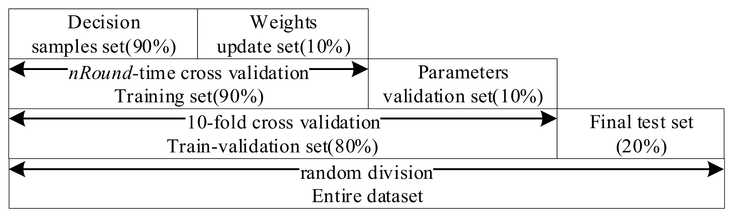
Unlike the traditional KNN algorithm, the improved algorithm presented in this paper involves a training process. Therefore, not only to compare with the target point for distance calculation, the training data needs to be divided for updating the weights. For clarity, the two training sets are called the decision samples set and the weights update set.

As shown in Algorithm 2, there are several input parameters: trainData is the data used for training, k is the k value of WKNN, nRound is the number of rounds for training, raDiv is the ratio for dividing the training samples into the decision samples set and the weights update set, and $\delta$ is an adjustment parameter used to calculate the feature selection threshold. It finally outputs the indexes of the selected features and the corresponding feature weights. The algorithm runs two times automatically by judging whether the value of $\delta$ is null. The first time is to select a feature set with no null $\delta$ and the second is to train the feature weights for the new features with null $\delta$.

First, in lines 1–3, WKNN-Selfada initializes the selected feature index set, selectedFeatureIndex, as all feature indexes, i.e., {0, ..., m−1}. Then it uses the function DataProcessing() to extract the feature values of the data according to the selected feature and initializes the feature weights, w, as values of 1/m, where m is the feature dimension.

Next, in lines 4–22, it loops several times at the value of nRound. At the beginning of each round, the method starts with a data division function, dataDivide(), which proportionally divides trainData into a decision samples set P and a weights-update set Q in the ratio raDiv. One training round involves multiple instances of training, which is equal to the size of the weights-update set Q. Line 7 implements the WKNN algorithm on decision sample set P and the weights-update sample q and yields the class prediction named prediction, the weighted feature-based point distances of the k-nearest decision samples, kDistances, the matrix of feature distances between each k-nearest decision samples and q, KFD, and the classes of the k-nearest decision samples, kClass. Then, it judges whether the prediction class is true. If false, it then implements the feature weights-update, which judges in sequence whether the class of each nearest k decision sample is equal to the true class of target point q. If not, the algorithm starts to update the weights, as shown in lines 11–17. In the phase of weights update, the process in the class of the ith k-nearest decision sample is different from the target sample, which is described below.

Algorithm 2: WKNN-Selfada

• Step 1: obtain the ranks of each feature based on the feature distances ${kfd}^{\left(i\right)}$. For example, if ${kfd}^{\left(i\right)}=(0.9,0.2,0.4)$, the ranks of the features are (3,1,2), where the ith element of rank means the rank of the ith feature according to the feature distance from small to large.
• Step 2: obtain the parameter $\lambda$, which is the update ratio of the weights. It is set to the ratio of the smallest weighted feature-based point distance in this loop, min(kDistances), to the weighted feature-based point distance between this decision sample and the target sample, kDistances[i].
• Step 3: calculate the denominator of the new weights, $\beta$. The denominator increment is given by $\Delta \beta =\lambda ·\frac{m(m+1)}{2}$, where $\lambda$ is the update ratio and m is the dimension of the feature vector. Thus, the new denominator is $\beta \leftarrow \beta +\Delta \beta$.
• Step 4: calculate the molecular of the new weights, $\alpha$. The molecular increments are given by ${\Delta \alpha }_i=\lambda ·\mathit{rank}\left[i\right]$, where i is the feature index. Thus, the new molecular are ${\alpha }_i\leftarrow {\alpha }_i+{\Delta \alpha }_i$, where ${\alpha }_i$ is the weight’s molecular of the ith feature.
• Step 5: calculate the new feature weights, $w={(w}_1{;\dots ;w}_m)\leftarrow (\frac{{\alpha }_1}{\beta };\dots ;\frac{{\alpha }_m}{\beta })$. The sum of all weights equal to 1 under any situation.

The misclassified decision sample at a shorter distance from the test point produces a larger update ratio $\lambda$, which means that it has a greater influence on the training process for feature weight update. After additional rounds of processing the feature weight self-adaptively, each feature weight converges to a certain value. In particular, if the influence of one feature is extremely low (or extremely high), the weight will converge to $2/[m·(m+1)] (\mathrm{or} 2/(m+1))$.

Then, in lines 23–31, the algorithm determines whether feature selecting is finished by judging whether $\delta$ is null. As $\delta$ does not have a null value in the first iteration, the processing of feature selection would be performed, i.e., lines 24–28. The algorithm selects the features by judging whether the weight of each feature is smaller than the feature selection threshold, ranging from the 1st dimension to the mth dimension in order. If so, the feature index corresponding to the weight is removed from selectedFeatureIndex. The threshold is obtained by calculating the difference between the average value of the weights, 1/m and $\delta$ times the standard deviation of the weights. Here, $\delta$ is an adjustable parameter and std() is the standard deviation function. The basic idea behind the threshold design is that the feature weights obey normal distribution, so values lower than the confidence intervals are rare and have low influences on the classification. In statistics, once the mean and standard deviation of the data are given, the $\delta$ can be determined based on the confidence level such as 95%, and the confidence intervals can be calculated, so values lower than the intervals can be removed. However, WKNN-Selfada does not use the notion of confidence level, but sets the $\delta$ and the threshold by experimental verification instead. At the end of the first iteration, the algorithm sets the $\delta$ to null and then begins the second iteration from line 2. In the second iteration, it calculates the new weights of the new feature according to the selectedFeatureIndex, shown in lines 4–22. After finishing the weight update, the algorithm ends up in the $\delta$ of null value, and outputs the feature indexes of the new feature set, selectedFeatureIndex, and the corresponding new feature weights, $w$.

4. Fine-Grained Classification of Encrypted Network Flows

This section proposes a fine-grained classification framework for encrypted traffic classification, which includes network flow division, flow feature extraction, fined-grained label designation, model training, and real-time classification. Based on this framework and the improved KNN algorithms presented in Section 3, a new method is proposed to realize fine-grained classification of encrypted network flows.

4.1. Description of Classification Framework

The main idea of the framework for fine-grained classification of encrypted network flows is to train three classifiers using the hierarchical features and classes of sample traffic data and use them to predict the fine-grained labels of real-time network flows. The framework is shown in Figure 2.

The framework consists of two parts: offline training and online classification. The offline part selects the hierarchical features and trains the corresponding feature weights of the three-layer model on the basis of the WKNN-Selfada algorithm after the processe of flow division and class extraction. The online part divides the flows from real-time traffic, extracts the flow features, and calculates the fine-grained classification result on the basis of the training model. The classification model calculates the point distances using the WKNN algorithm.

The key aspect of the framework is the fine-grained three-layer classifier model. The first layer is the traffic encryption status identification layer, which is the basis of the entire framework. It identifies an encrypted flow through the feature set of the encryption status. The identified encrypted flow then undergoes fine-grained analysis, i.e., it enters the second and third layers of the model. The second layer is the application identification layer for encrypted flows. The feature set of application type is used to identify the application to which the encrypted network flow belongs. The third layer is the content type identification layer. The feature set of content type is used to identify the content type (such as files, simple communication messages, audio and video communication, or multimedia streams) transmitted by the encrypted application flow, which undergoes further fine-grained analysis for the encrypted flow.

Combining with the analysis of the correlations of the fine-grained results and the secure rules, a more effective network defense would be implemented. For example, a malicious flow simulated as the YouTube flow, is detected as a YouTube and file flow by the framework. If we just analyze a single attribute value of the flow, e.g., YouTube or file, the malicious flow would be regarded as normal flow, which would cause damage to the network. However, if we analyze the correlations of the attributes and match the secure rule such as “If a YouTube flow is a file flow, the flow is suspicious.”, the malicious flow would attract the network manager’s attention and further be prevented from damage.

4.2. Design of Candidate Feature Set

The hierarchical feature set of the framework is based on the feature selection part of the WKNN-Selfada algorithm, which selects features from the candidate feature set shown in

Table 1. Description of candidate flow feature set.

	Feature	Calculation Formula
1	Minimum of packet inter-arrival time	iat_min = min(iat[])
2	Maximum of packet inter-arrival time	iat_max = max(iat[])
3	Mean of packet inter-arrival time	iat_mean = mean(iat[])
4	Standard deviation of packet inter-arrival time	iat_std = std(iat[])
5	Minimum of IP packet bytes	byte_min = min(byte[])
6	Minimum of IP packet bytes	byte_max = max(byte[])
7	Mean of IP packet bytes	byte_mean = mean(byte[])
8	Standard deviation of IP packet bytes	byte_std = std(byte[])
9	Number of IP packet bytes per second	byte_psec =$\frac{{{\displaystyle \sum }}_{i=1}^{n}byte\left[i\right]}{{{\displaystyle \sum }}_{i=1}^{n}iat\left[i\right]}$
10	Number of packets per second	pac_psec =$\frac{n}{{{\displaystyle \sum }}_{i=1}^{n}iat\left[i\right]}$
11	Minimum of forward packet inter-arrival time	fiat_min = min(fiat[]), $\mathrm{fiat}=\left\{\mathrm{iatsd}\right[i\left]\right|d\left[i\right]==0\}$[]
12	Maximum of forward packet inter-arrival time	fiat_max = max(fiat[])
13	Mean of forward packet inter-arrival time	fiat_mean = mean(fiat[])
14	Standard deviation of forward packet inter-arrival time	fiat_std = std(fiat[])
15	Minimum of IP packet bytes of forward packets	fbyte_min = min(fbyte[]), $\mathrm{fbyte}=\left\{\mathrm{byte}\right[i\left]\right|d\left[i\right]==0\}$[]
16	Minimum of IP packet bytes of forward packets	fbyte_max = max(fbyte[])
17	Mean of IP packet bytes of forward packets	fbyte_mean = mean(fbyte[])
18	Standard deviation of IP packet bytes of forward packets	fbyte_std = std(fbyte[])
19	Number of IP packet bytes of forward packets per second	fbyte_psec =$\frac{{{\displaystyle \sum }}_{i=1}^{n_{fp}}fbyte\left[i\right]}{{{\displaystyle \sum }}_{i=1}^{n_{fp}}fiat\left[i\right]}$
20	Number of forward packets per second	fpac_psec =$\frac{n_{fp}}{{{\displaystyle \sum }}_{i=1}^{n_{fp}}fiat\left[i\right]}$
21	Minimum of backward packet inter-arrival time	biat_min = min(biat[]), $\mathrm{biat}=\left\{\mathrm{iatsd}\right[i\left]\right|d\left[i\right]==1\}$[]
22	Maximum of backward packet inter-arrival time	biat_max = max(biat[])
23	Mean of backward packet inter-arrival time	biat_mean = mean(biat[])
24	Standard deviation of backward packet inter-arrival time	biat_std = std(biat[])
25	Minimum of IP packet bytes of backward packets	bbyte_min = min(bbyte[]), $\mathrm{bbyte}=\left\{\mathrm{bbyte}\right[i\left]\right|d\left[i\right]==1\}$[]
26	Minimum of IP packet bytes of backward packets	bbyte_max = max(bbyte[])
27	Mean of IP packet bytes of backward packets	bbyte_mean = mean(bbyte[])
28	Standard deviation of IP packet bytes of backward packets	bbyte_std = std(bbyte[])
29	Number of IP packet bytes of backward packets per second	bbyte_psec =$\frac{{{\displaystyle \sum }}_{i=1}^{n_{bp}}bbyte\left[i\right]}{{{\displaystyle \sum }}_{i=1}^{n_{bp}}fiat\left[i\right]}$
30	Number of backward packets per second	bpac_psec =$\frac{n_{bp}}{{{\displaystyle \sum }}_{i=1}^{n_{bp}}fiat\left[i\right]}$
31	Number of forward packets for the first 10 packets	$n_{\mathrm{fp}}^{\left(10\right)}={\displaystyle {\displaystyle \sum }_{i=1}^{10}}(1 \mathrm{if} d\left[i\right]==0 \mathrm{else} 0)$
32	Number of backward packets for the first 10 packets	$n_{\mathrm{bp}}^{\left(10\right)}={\displaystyle {\displaystyle \sum }_{i=1}^{10}}(1 \mathrm{if} d\left[i\right]==1 \mathrm{else} 0)$
33	Number of forward packets for the first 60 packets	$n_{\mathrm{fp}}^{\left(60\right)}={\displaystyle {\displaystyle \sum }_{i=1}^{10}}(1 \mathrm{if} d\left[i\right]==0 \mathrm{else} 0)$
34	Number of backward packets for the first 60 packets	$n_{\mathrm{bp}}^{\left(60\right)}={\displaystyle {\displaystyle \sum }_{i=1}^{10}}(1 \mathrm{if} d\left[i\right]==1 \mathrm{else} 0)$
35	Ratio of the number of backward packets to forward packets for the first 10 packets	$r_p{}^{\left(10\right)}=\frac{n_{\mathrm{bp}}^{\left(10\right)}}{n_{\mathrm{fp}}^{\left(10\right)}}$
36	Ratio of the number of backward packets to forward packets for the first 60 packets	$r_p{}^{\left(60\right)}=\frac{n_{\mathrm{bp}}^{\left(60\right)}}{n_{\mathrm{fp}}^{\left(60\right)}}$

. In the field of traffic classification, traffic features can be classified as packet features and flow features. Packet feature extraction is relatively simple and efficient, but its classification accuracy is low. Furthermore, the analysis of flow features is complicated. However, as network flows can be regarded as basic units of network behavior between pair-wise subjects, the analysis based on flow features is more comprehensive in the area of network traffic and it achieves higher classification accuracy. The definition of network flow is as follows. In this paper, flow refers to bilateral flow unless otherwise specified.

Definition 4 (Network flow).

Network flow is a set of packets with the same five-tuple (source IP, destination IP, source port, destination port, transport protocol) in the same network in a certain period of time.

Definition 5 (Bilateral flow).

Bilateral flow is a pair of flows having symmetrical source IP, source port, destination IP, and destination port in the same network in a certain period of time.

In the previous studies, static features such as IP, port number, and TCP (Transmission Control Protocol) flags were used as part of the feature set [67], which reduces the robustness of the classification model. When the model is trained with the traffic of a certain network, it will not perform well on another network or in another period of the network. Considering portability and robustness for encrypted traffic classification, this study extracts only spatio-temporal statistical flow features, including the interval of packets, bytes of packets, count of packets, ratio of packets, and velocity of flow, instead of static features. These features are extracted from two directions of the entire flow (forward and backward) and four statistical dimensions (minimum, maximum, mean, and standard deviation). Table 1 shows that functions of $\min \left(\right), \max \left(\right), \mathrm{mean}\left(\right) \mathrm{and} \mathrm{std}\left(\right)$ are to obtain the minimum, maximum, average and standard deviation value of the array, respectively. byte[] is an array of the number of IP packet bytes, where byte[i] means the length of the ith IP packet bytes. iat[] is an array of interval arrival time between the two adjacent packets, where iat[i] means the time interval between the ith packet and the i+1th packet. iatsd[] is an array of the inter-arrival time of packets in the same direction. d[] is an array of the directions of packets. n, $n_{fp}$, $n_{bp}$ are the number of the all packets, forward packets and backward packets in a flow, respectively, where the maximum is 60. Because the extracted flow features are based on the first 60 packets of a flow at most, it decreases the calculation cost.

It is worth noting that when selecting the candidate feature set, this study adds the number and the proportion of packets from different directions of the first 10 or 60 packets of one flow as features, as indicated in features of 31–36. The first several packets of one flow always represent the important interaction or negotiation between the two hosts, which indicates the key characteristics of the traffic. Using these features can improve the accuracy of network traffic identification. The experiments in this study also prove that these features play a significant role in application type and content type identification for encrypted network flows.

4.3. Fine-Grained Classification Method

Based on the developed framework and the WKNN algorithm, this section proposes a fine-grained classification method for encrypted traffic on the basis of the improved KNN algorithm (FCE-KNN), which is shown in Algorithm 3. FCE-KNN includes two parts: model training and real-time classification. Furthermore, several definitions related to the algorithm are given below.

Definition 6 (FCE flow label).

The label of the network flow in each layer of the fine-grained framework is called the FCE flow label. The ith layer label value of flow is$L_i\left(\mathit{flow}\right)$.

Definition 7 (FCE feature index).

After training and selection, the feature indexes set used for real-time classification in the framework are denoted by FI.

Lines 1–5 are the offline model training part of FCE-KNN, which is based on the WKNN-Selfada algorithm. It sets the ratio of data division raDiv to 9, which means that the algorithm uses 90% of the training samples as the decision-sample set and the remaining 10% as the weight-update set in each training round. As the value of nRound does not exceed the ratio range from the size of the complete set to the size of the weights update training set, the model can avoid overfitting as much as possible. Overfitting is one of the main problems in machine learning. It means that the model completely learns the characteristics of the training data, but cannot generalize the laws in other data. Because of the right setting of nRound and raDiv, each training data would not be reused as a weight update sample and the characteristics of each weight update sample would just be learned once. Thus, it avoids the over-learning situation that the model learns the characteristics of the same training data repeatedly, which may lead to difficulties of model generalization. Data normalization is a useful means to process data and is able to speed up the model training. In this paper, for a certain feature dimension, the new feature value of the ith data is given by $x_i’=\frac{x_i-\mu \left(x\right)}{\sigma \left(x\right)}$, where $x_i$ is the old feature value; $\mu \left(x\right)$ is the mean; $\sigma \left(x\right)$ is the standard derivation; and $x_i’$ is the new feature value.

Algorithm 3: FCE-KNN

As shown in lines 3–5, the training part calculates the selected feature sets and feature weight sets of the sub-classifier models on the basis of the WKNN-Selfada algorithm. As for the parameters, k₁, k₂, k₃; nRound₁, nRound₂, nRound₃; and ${\delta }_1{, \delta }_2{, \delta }_3$ are the values of k, nRound and $\delta$ of the WKNN-Selfada algorithm implemented in each layer classification task, respectively. Furthermore, trainFlows represents the flow features of the training samples after data normalization, while enTrainFlows represents the encrypted flow data of trainFlows. The sets of ${\mathit{FI}}_1{, \mathit{FI}}_2{ \mathrm{and} \mathit{FI}}_3$ are the selected feature index, while $w^{\left(1\right)}{, w}^{\left(2\right)}{ \mathrm{and} w}^{\left(3\right)}$ are the feature weight sets after training.

When the training phase ends, all the sample data will be used as the decision samples in the online phase to calculate the point distance from the test point and determine its class.

Lines 6–22 are the real-time classification part of FCE-KNN, including real-time network flow mapping, flow feature real-time update, and flow label calculation based on WKNN. The model first extracts the five-tuple information, packet length, and timestamp of every online packet. The five-tuple is used to map the online packet to a certain flow, ${\mathit{Flow}}^{(i)}$, and the length of ${\mathit{Flow}}^{(i)}$ is increased by 1. The function featureUpdate() implements flow feature real-time update for ${\mathit{Flow}}^{(i)}$ on the basis of the length of the packet, len(packet), and the timestamp, t(packet). As FCE-KNN extracts flow features from only the first 60 packets of each flow, the algorithm first judges whether the packet number of the flow reaches 60 in each instance. If the number does not exceed 60, the algorithm will use len(packet) and t(packet) of the processing packet to implement the flow feature update. Then, the algorithm will judge whether the packet number of the flow exceeds 60 or whether the flow is over. If so, the algorithm enters the label calculation part, as shown in lines 13–20. In this part, feature data normalization is the first operation to be implemented. Then, according to the selected feature index sets, ${\mathit{trainFlows}}_1{, \mathit{entrainFlows}}_2{ \mathrm{and} \mathit{entrainFlows}}_3$ are extracted as the training data for the different sub-models classification of the new flow, respectively. Similarly, ${\mathit{Flow}}_1^{(i)}{,\mathit{Flow}}_2^{(i)}{,\mathit{Flow}}_3^{(i)}$ are the extracted features of the target data, respectively. The first sub-classifier is used to identify the encryption status, i.e., $L_1{(\mathit{Flow}}^{(i)})$. If it is an encrypted flow, the second and third sub-classifiers are used to identify the application type $L_2{(\mathit{Flow}}^{(i)})$ and content type $L_3{(\mathit{Flow}}^{(i)})$, respectively. Finally, the algorithm outputs the fine-grained classification result. Note that if the classification result of the first sub-classifier is non-encrypted, the algorithm will directly output this classification result.

5. Experiments and Evaluation

This section describes experiments based on the FCE-KNN method and compares the fine-grained classification performance of FCE-KNN with that of other, similar algorithms.

5.1. Setup

The experimental platform was an MSI GT63 laptop with a six-core central processing unit (CPU, Intel Core i7-8750; 2.2 GHz) and 16 GB RAM. Experiments were performed on the public dataset ISCX VPN-nonVPN [16]. The public dataset used in this paper was captured in in-network routers, which was a representative dataset of real-world traffic generated by ISCX. The data in the dataset were raw traffic, without any preprocessing. The algorithms were implemented in Python.

The model needs to perform fine-grained analysis of application type and content type for encrypted traffic, and only the ISCX VPN-nonVPN dataset can meet the experimental requirements of this study on public datasets. Therefore, experiments were performed only on this dataset. The size of the ISCX VPN-nonVPN dataset is 25 GB, of which 22.8 G is plaintext traffic and the remaining 2.4 GB is encrypted traffic generated using VPN. The dataset contains 280,540 flows, of which 18,468 are ciphertext flows and 262,072 are plaintext flows, including 14 types of applications, covering a wide range of applications as well as multiple content types. Therefore, we used this dataset in our study.

To meet the experimental requirements, we added fine-grained classes for flows based on the dataset, so that the dataset can be used in the experiments. After class adjustment, each flow contains three classes (encryption status, application type, content type). The number of flows with different classes was summarized in

Table 2. Flow labels and number of flows used in the experiments.

Label Type	Label Name and Number
Encryption Status	Encrypted (18468)		Non-Encrypted (262072)
Application type (Encrypted flows)	AIM (32)	Email (298)
	ICQ (31)	FTPS (125)
	VoipBuster (1618)	Facebook (2494)
	Spotify (137)	BitTorrent (477)
	Hangouts (10871)	Netflix (173)
	YouTube (213)	Skype (1835)
	SFTP (28)	Vimeo (136)
Content type (Encrypted flows)	Chat (4327)	File (1497)
	VoIP (11,985)	Streaming (659)

. Note that in the classification tasks of the second and third layers, FCE-KNN only analyzes encrypted flows. The application label types include AIM (AmericanOnline Instant Messenger), ICQ (I Seek You, one of the message software), VoipBuster (one of the voice communication software), Spotify (one of the music service software), Hangouts (one of the message software), Youtube (one of the video communication software), SFTP (SSH File Transfer Protocol), Email, FTPS (File Transfer Protocol over SSL (Secure Sockets Layer)), Facebook (one of the message software), BitTorrent (one of the file transfer software), Netflix (one of the video communication software), Skype (one of the message software) and Vimeo (one of the message software). The content label types include chat, VoIP, file and streaming.

To test the performance of FCE-KNN, the dataset was divided into a train-validation set and test set. The test set was only used for the final performance test of the model. Meeting the need of parameters’ validation, 10-fold cross-validation was used to improve the utilization of the train-validation set. To satisfy the requirement for the algorithms, the model training data of the train-validation set was further divided into a decision samples set and a weights update set in each fold of cross-validation. The details of the data division is shown in Figure 3.

Although we have said that the analysis of the fine-grained classification of encrypted flows can be used for anomaly detection, we did not evaluate the performance. On the one hand, the main proposal of our research is to analyze encrypted network flows, but not to detect malicious flows, so we had not considered evaluating the anomaly detection effect of the presented method. On the other hand, anomaly detection based on the analysis of correlations between the flow attributes is a little subjective. There is not a suitable public dataset that can be used, and if we create a dataset that regards some flows with specific application and content to be malicious according to our judgement, and evaluate the presented method on this dataset, the results make no sense. This is because the malicious flows are designed by ourselves and we know the rules of anomaly in advance. Therefore, testing the performance of identifying the application and content type of encrypted flows is a more essential, useful and effective evaluation. As long as we identify the fine-grained attributes of the network flows, we can easily find out the malicious flows with strange combinations of application type and content type according to the network security rules.

5.2. Metric

The following metrics were used to evaluate the classification effect: Accuracy, Precision, Recall, and F1-Score. The metrics are defined as: $\mathit{Accuracy}=\frac{{\mathit{TP}}_i}{{\mathit{TP}}_i{+\mathit{FN}}_i}$, $\mathit{Precision}=\frac{{\mathit{TP}}_i}{{\mathit{TP}}_i{+\mathit{FP}}_i}$, $\mathit{Recall}=\frac{{\mathit{TP}}_i}{{\mathit{TP}}_i{+\mathit{FN}}_i}$ and $F1-\mathit{score}=\frac{2·\mathit{Precision}·\mathit{Recall}}{\mathit{Precision}·\mathit{Recall}}$. Among them, TP_i is the number of ith type flows that are correctly classified, FP_i is the number of not ith type flows that are misclassified as ith type flows, and FN_i is the number of ith type flows that are misclassified as not ith type flows. In the first-layer classification, which was a two-class task, the types of flows are encrypted and non-encrypted. In the second and third layers of classifications, i.e., multi-class tasks, the types of flows are different application (content), e.g., FTPS, Email etc. (Chat, File etc.).

5.3. Experiments and Results

Some important parameters of FCE-KNN are k, nRound, and $\delta$. This section discusses the classification performance analysis of FCE-KNN and evaluates the optimal values of the parameters. According to the three classification layers in FCE-KNN, this section is divided into three subsections, including analyzing the performance of FCE-KNN in identifying the encryption status, application type, and content type of encrypted flows, respectively. The four state-of-the-art methods, including DTW-KNN (Dynamic Time warping based on KNN) [53], C4.5 (one of the decision trees) [16], ADA (ADAboost, one of the ensemble method) [32] and AISVM (Incremental Support Machine with Attenuation factor) [31] are compared with FCE-KNN. DTW-KNN [53] is a variant KNN, which is based on the optimization problem, dynamic time warping, with the minimum cumulative distance when the two templates are matching. ADA [32] is an ensemble machine learning algorithm, adaboost, which is an ensemble classifier with multiple simple C4.5. C4.5 [16] is one of the widely used decision tree algorithm. AISVM [31] isa modified version of the incremental support vector machine (ISVM), which introduces attenuation factor and improves accuracy. All the algorithms in comparison are network traffic-classification methods based on modified versions of machine-learning algorithms. Neural networks are also widely used in traffic classification, but they need large amount of training data, which make no sense in evaluation with a small training set.

5.3.1. Identification of Encryption Status of Network Flows

This section verifies the performance of FCE-KNN in identifying the flow encryption status, i.e., whether a flow is an encrypted flow or not.

The optimal parameter values were first analyzed. As shown in Figure 4a, k₁ is most likely to obtain an optimal value between 1 and 21. As shown in Figure 4b, when k₁ is 5, the accuracy reaches the highest, which is 99.14%. The analysis of the optimal nRound₁ value is shown in Figure 5a. As nRound₁ increases, the verification accuracy of the model changes accordingly. In the 3rd and 8th rounds, the testing accuracy reaches its highest value without over-fitting. Considering that the three-round training requires a shorter training time, the best value for nRound₁ is 3. The analysis of the optimal ${\delta }_1$ value is shown in Figure 5b. When the value is 0.6 or 0.8, the accuracy of the model is the highest, and as the value increases, the accuracy decreased significantly. Therefore, a value of 0.6–0.8 is relatively suitable. The experiment also outputs the feature weights in the feature selection part of the model training, as shown in Figure 6, where the red line indicates the feature selection threshold. It can be seen that the features of the packet interval and packet byte have a significant impact on the classification. The trained model retains only around 1/3 of all the features, further indicating that the reduction in traffic features can improve not only the efficiency of online feature extraction but also the classification accuracy.

In this section, two sub-experiments were implemented. The first one was to train a model on the whole train-validation set and test the model on the test set. To verify the robustness of FCE-KNN for flow encryption status identification, the other one was performed to test whether the model can deal with the flows of an unknown application. In this experiment, assuming Hougout was an unknown application, we used all the data except Hougout flows and the corresponding encryption status labels to train a model, and tested the model on the all Hougout flows.

The parameter setting of FCE-KNN was as follows: k₁ was set to 3, nRound₁ was set to 3, and ${\delta }_1$ was set to 0.6. As shown in

Table 3. Performance comparison between FCE-KNN and other algorithms for identifying the encryption status of network flows.

Method	Test on Known-Application Flows				Test on Unknown-Application Flows
	Acc (%)	Pre (%)	Rec (%)	F1	Acc (%)	Pre (%)	Rec (%)	F1
FCE-KNN	99.34	98.56	91.31	0.94	99.30	99.37	94.69	0.96
DTW-KNN [53]	98.99	96.71	87.68	0.91	98.20	94.46	90.12	0.92
C4.5 [16]	98.99	98.12	86.27	0.91	98.96	99.67	91.51	0.95
ADA [32]	99.11	97.87	88.41	0.92	99.06	99.99	92.08	0.95
AISVM [31]	95.01	59.17	78.01	0.67	88.10	45.94	0.31	0

Acc is Accuracy; Pre is Precision of identification of encrypted flows; Rec is Recall of identification of encrypted flows; F1 is F1-score of identification of encrypted flows.

, FCE-KNN exhibited the best performance. Although the performance of FCE-KNN was not significantly better than that of the other algorithms, the precision and recall of FCE-KNN were high in the case of unbalanced classes, which indicated that FCE-KNN was sensitive to encrypted flows. Note that it was not easy to maintain high precision and high recall at the same time. Thus, FCE-KNN has high adaptability to encrypted flows classification tasks. In addition, it performed best at identifying the encryption status of the unknown application flows, showing the best robustness of classification.

5.3.2. Identification of Application Type of Encrypted Network Flows

This section tests the performance of FCE-KNN in the application type classification of encrypted flows, i.e., what type of application is used. According to the dataset ISCX VPN-nonVPN, flows used in the experiment involve 14 types of applications: AIM, BitTorrent, email, Facebook, FTPS, Hangouts, ICQ, Netflix, SFTP, Skype, Spotify, Vimeo, VoipBuster, and YouTube.

First, paraments validation were implemented. As shown in Figure 7, the accuracy reaches its maximum value when k₂ is equal to 11, and as k₂ increased, the accuracy gradually decreases. When k₂ is 8, the accuracy is the highest, which is 91.61%. The analysis of the optimal nRound₂ value is shown in Figure 8a. As nRound₂ increases, the validation accuracy of the model does not change significantly. It can be seen that the feature weights have been trained to converge in the first round; hence, the optimal value of nRound₂ is 1. The analysis of the best ${\delta }_2$ value is shown in Figure 8b. The model achieves the highest accuracy of 91.68% at a value of −0.2. As the value increases, the accuracy decreases significantly. This is because there are only two or three features left in the selected feature set, which degraded the classification performance severely. Figure 9 shows all the feature weights in the feature selection part of the model training. The trained model retains only around half of the features, and the feature of packet byte plays an important role in the application-type identification of encrypted flows.

In this experiment, for the parameters of FCE-KNN, k₂ was set to 8, nRound₂ was set to 1, and ${\delta }_2$ was set to −0.2. As shown in

Table 4. Accuracy comparison between FCE-KNN and other algorithms for identifying application type of encrypted network flows.

Method	Accuracy (%)
FCE-KNN	92.45
DTW-KNN [53]	90.06
C4.5 [16]	85.71
ADA [32]	89.77
AISVM [31]	67.65

,

Table 5. Precision comparison between FCE-KNN and other algorithms for identifying application type of encrypted network flows.

Method	Precision (%)
	AIM	BitTorrent	Email	Facebook	FTPS	Hangouts	ICQ
FCE-KNN	66.66	93.54	82.35	89.13	80.76	96.40	33.33
DTW-KNN [53]	0	86.95	78.18	86.91	45.71	95.78	0
C4.5 [16]	0	77.77	0	96.06	0	95.04	0
ADA [32]	0	85	87.5	82.79	84.61	95.39	0
AISVM [31]	0	0	0	0	0	72.02	0
Method	Precision (%)
	Netflix	SFTP	Skype	Spotify	Vimeo	VoipBuster	YouTube
FCE-KNN	52.5	0	83.84	45.45	50	98.15	83.33
DTW-KNN [53]	29.41	0	76.22	35.29	60	98.70	70.73
C4.5 [16]	62.5	0	47.39	41.66	0	95.93	0
ADA [32]	59.25	0	72.41	57.14	32.60	97.22	80
AISVM [31]	0	0	28.69	0	0	84.59	0

,

Table 6. Recall comparison between FCE-KNN and other algorithms for identifying application type of encrypted network flows.

Method	Recall (%)
	AIM	BitTorrent	Email	Facebook	FTPS	Hangouts	ICQ
FCE-KNN	33.33	91.57	93.33	87.17	84	97.33	16.66
DTW-KNN [53]	0	84.21	71.66	85.17	64	97.19	0
C4.5 [16]	0	66.31	0	73.34	0	96.27	0
ADA [32]	0	71.57	70	87.77	44	97.24	0
AISVM [31]	0	0	0	0	0	96.18	0
Method	Recall (%)
	Netflix	SFTP	Skype	Spotify	Vimeo	VoipBuster	YouTube
FCE-KNN	60	0	82.01	37.03	59.25	98.45	69.76
DTW-KNN [53]	42.85	0	76.02	44.44	33.33	94.44	67.44
C4.5 [16]	14.28	0	89.10	18.51	0	94.75	0
ADA [32]	45.71	0	74.38	29.62	55.55	97.22	37.20
AISVM [31]	0	0	34.87	0	0	86.41	0

and

Table 7. F1-score comparison of FCE-KNN for identifying application type of encrypted network flows with other algorithms.

Method	F1-Score
	Aim	Bittorrent	Email	Facebook	Ftps	Hangouts	Icq
FCE-KNN	0.44	0.92	0.87	0.88	0.82	0.96	0.22
DTW-KNN [53]	0	0.85	0.74	0.86	0.53	0.96	0
C4.5 [16]	0	0.71	0	0.83	0	0.95	0
ADA [32]	0	0.77	0.77	0.85	0.57	0.96	0
AISVM [31]	0	0	0	0	0	0.83	0
Method	F1-Score
	Netflix	Sftp	Skype	Spotify	Vimeo	Voipbuster	Youtube
FCE-KNN	0.56	0	0.82	0.40	0.54	0.98	0.75
DTW-KNN [53]	0.34	0	0.76	0.39	0.42	0.96	0.69
C4.5 [16]	0.23	0	0.61	0.25	0	0.95	0
ADA [32]	0.51	0	0.73	0.39	0.41	0.97	0.50
AISVM [31]	0	0	0.31	0	0	0.85	0

, FCE-KNN shows the best performance in the application type identification of encrypted flows and the highest accuracy among the five algorithms, with an improvement of 2.4% over the second-ranked algorithm (DTW-KNN). AISVM performed well in Section 5.3.1, but it did not seem to perform well in multi-class tasks. In most of the classes, FCE-KNN has the highest Precision, Recall, and F1-score. Furthermore, we found that it was difficult to identify the flows of AIM, ICQ, and SFTP, mainly because the amount of flows of these classes was too small to train the model, whereas the number of training data of AIM, ICQ and SFTP were 24, 24 and 22, respectively. Nevertheless, FCE-KNN could correctly classify some of them such as AIM and ICQ, which performed better than other algorithms. Thus, FCE-KNN can rapidly adapt to the environment in the condition of imbalanced classes and small training set. Furthermore, note that FCE-KNN has the highest F1 scores in all the classes, which has fairly good stability, i.e., it balanced the precision and recall.

5.3.3. Identification of Content Type of Encrypted Network Flows

This section tests the performance of FCE-KNN in identifying the content type of encrypted flows, i.e., what type of content is carried by the encrypted flows. According to the public dataset ISCX VPN-nonVPN and subsequent manual marking, the flows used in the experiment include four types of content: chat, file, VoIP, and streaming.

First, paraments validation were implemented. As shown in Figure 10, the accuracy reaches its maximum value when k₃ is equal to 11, and as k₃ increases, the accuracy gradually decreases. When k₃ is 1, the accuracy is the highest, which is 96.67%. The analysis of the optimal nRound₃ value is shown in Figure 11a. As nRound₃ increases, the accuracy of the model does not change significantly. It can be seen that feature weights have been trained to converge in the first round; hence, the optimal value of nRound₃ is 1. The analysis of the best ${\delta }_3$ value is shown in Figure 11b. The model has the highest testing accuracy when ${\delta }_3$ is 0, where the feature selection threshold is the mean of all the feature weights. Figure 12 shows all the feature weights in the feature selection part of the model training. The trained model retains only around half of the features, and the features of packet interval and packet byte have significant influence on the model classification.

The performances of FCE-KNN and the other algorithms are summarized in

Table 8. Accuracy comparison between FCE-KNN and other algorithms for identifying content type of encrypted network flows.

Method	Accuracy (%)
FCE-KNN	97.02
DTW-KNN [53]	94.50
C4.5 [16]	92.69
ADA [32]	95.37
AISVM [31]	66.00

and

Table 9. Performance comparison between FCE-KNN and other algorithms for identifying content type of encrypted network flows.

Method	Chat			File			Streaming			VoIP
	P(%)	R(%)	F1	P(%)	R(%)	F1	P(%)	R(%)	F1	P(%)	R(%)	F1
FCE-KNN	95.78	96.99	0.96	88.85	90.63	0.89	91.72	92.42	0.92	98.82	98.08	0.98
DTW-KNN [53]	93.68	94.22	0.93	82.43	81.60	0.82	80.62	78.78	0.79	97.03	97.07	0.97
C4.5 [16]	97.64	91.10	0.94	64.10	83.61	0.72	82.14	52.27	0.63	96.01	96.62	0.96
ADA [32]	97.04	94.80	0.95	80.93	80.93	0.80	83.33	75.75	0.79	97.15	98.45	0.97
AISVM [31]	0	0	0	50.30	27.42	0.35	0	0	0	66.74	98.28	0.79

P is Precision; R is Recall; F1 is F1-score.

. The parameter setting of FCE-KNN was as follows: k₃ was set to 1, nRound₃ was set to 1, and ${\delta }_3$ was set to 0. It can be seen that the FCE-KNN also has the highest accuracy in the content type identification of encrypted flows, with an improvement of 2.7% over the second-ranked algorithm (ADA), and it has the highest F1-score in all the classes, indicating that FCE-KNN has high adaptability in identifying the content type of encrypted flows. Note that for the prediction of streaming flows, the performance of other algorithms are obviously lower than FCE-KNN by approximately 10%. The reason may be that the streaming flows does not have strong regularity, suggesting that FCE-KNN has excellent learning ability even if the data do not have strong regularity.

5.4. Analysis of Time Complexity and Consumption

It is important to analyze the complexity and time consumption of an algorithm. Low time-consumption is a significant requirement for real-time classification. FCE-KNN consists of WKNN and WKNN-Selfada algorithms. We first analyzed the time complexity of the algorithms. For WKNN, to predict the label of the test point, the algorithm will calculate the point distance between the test point and each decision training sample, so the time complexity is $O\left(m\right) \approx O\left(n\right)$, where m is the size of the decision sample set, and n is the size of the whole training set. For WKNN-Selfada, to select the features and obtain the corresponding feature weights, the algorithm will first calculate the point distance between the each weight’s update sample and each decision training sample, so the time complexity is $O(m·(n - m)) \approx O(n^2)$, where $n - m$ is the size of the weights update set. Accordingly, the training time complexity of FCE-KNN is $O(n^2)$, and the test time complexity is $\mathrm{O}\left(\mathrm{n}\right)$. In addition, the training time complexities of DTW-KNN, C4.5, ADA and AISVM are $O(n^2)$, $O\left(\log \right(n)·n)$, $O\left(\log \right(n)·n·k)$, $O(n^2)$, respectively, and the test time complexities are $O\left(n\right)$, $O\left(d\right)$, $O(d·k)$, $O\left(s\right)$, respectively, where k is the number of trees, d is the depth of the trees, and s is the number of the support vectors.

Then the actual time consumption is analyzed, as shown in

Table 10. Time consumption comparison between FCE-KNN and other algorithms in the framework of fine-grained classification (s).

Method	Training			Testing
	1st Layer	2nd Layer	3rd Layer	1st Layer	2nd Layer	3rd Layer
FCE-KNN	116.33	0.31	0.25	16.98	0.22	0.22
DTW-KNN [53]	77.15	0.20	0.17	15.71	0.20	0.19
C4.5 [16]	0.98	0.04	0.04	0.01	0.01	0.01
ADA [32]	206.93	10.75	9.45	0.73	0.15	0.07
AISVM [31]	1595.10	9.75	10.00	67.51	1.61	1.41

. The training numbers of the flows in the experiments of the three layers are 224,432; 14,774; and 14,774, respectively. The test numbers of the flows in the experiments of the three layers are 26,108; 3694; and 3694, respectively. The sizes of the selected feature sets of the three layers are 12, 19, 18. It could be seen that the time consumptions of FCE-KNN are a little high, just lower than ADA and AISVM. It is possible that FCE-KNN processes the feature selection and feature weights calculation, which is more time-consuming than traditional KNN. It is also because the algorithm learns the characteristics from each sample completely, consuming more time to train on a single sample. Thus, the total time consumption is a little higher than similar algorithms.

5.5. Discussion

It can be seen from the experimental results in Section 5.3 that FCE-KNN is not sensitive to the k value. FCE-KNN overcomes the drawbacks of the traditional KNN algorithm, i.e., it is more robust and shows better performance. Furthermore, FCE-KNN is not sensitive to nRound. This may be because the weight update samples are sufficient and the feature weights converge after the first round of training. For the threshold $\delta$ used for feature selection, the performance is stable before reaching the optimum value, and the accuracy of the model will decrease rapidly after a certain peak value. This may be because the size of the selected feature set will be extremely small, and there may be only two or three features when the value is large. From the curve of $\delta$, we can conclude that for traffic classification the feature set should not be as large as possible; redundant features may degrade the classification performance owing to the weak correlation with the classification target.

The performance of FCE-KNN is not always optimal in all the experiments. Although, the performance is not the best in a few cases of identification of a single class, the F1 scores are the highest in all the classes, indicating that FCE-KNN is a highly balanced algorithm with both high precision and high recall. Moreover, FCE-KNN has high practicability as it can identify the encryption status of unknown applications. In the experiments described in Section 5.3.2 and Section 5.3.3, FCE-KNN shows better performance than the other algorithms in the case of class imbalance, such as small amounts of ICQ, AIM, and Netflix flows in the task for identifying the application type of encrypted flows. For example, under the situation that the number of AIM flows was 32, the precision of FCE-KNN was 66%, while other algorithms were 0. To some extent, FCE-KNN alleviates the problem of class imbalance and small training set and shows strong adaptability to actual traffic environments. From the experimental results, it is seen that FCE-KNN performs better than those algorithms because different features have different influences upon different classification tasks and the presented algorithm has expressed the different influences by introducing feature weights self-adapting adjustment. It is proved that the thought of feature selection and feature weights self-adaption are effective and feasible.

As for the fact that FCE-KNN can train an accurate model with a small training set, we can evaluate this from two perspectives. On the one hand, the WKNN-Selfada algorithm selectes features by comparing the trained feature weights, and the feature weights are updated by a single training sample each time, not a batch. So it could fully learn the characteristics of each sample and train an accurate model just by using a small training set. This means that the algorithm adjusts the feature weights on each sample. In other words, every sample is beneficial and useful for the model training, which is different from some algorithms in which the model is trained on some special samples. On the other hand, in the experiments of identification of application type and content type of network flows, the number of some flows is very small, such as AIM, ICQ, FTPS, of which the numbers are 32, 31, 125, respectively. For those flows with a small amount, FCE-KNN shows obvious superiority comparing with other algorithms, which proves that FCE-KNN is able to train a model in the case of a small training set.

However, time consumption of FCE-KNN is a little higher than the other algorithms, which means more good hardware is required to achieve real-time classification. Owing to processes of feature selection and feature weights self-adaption, the time consumption of model training is high, but this did not affect the real-time processing. The feature extraction and distance calculation can be incrementally updated, where the raw packets do not need to be stored and the packet data can just be processed once. To sum up, FCE-KNN improves the traditional KNN algorithm and performs better than similar algorithms in accuracy, while it is a little time-consuming.

6. Conclusions

This study improves the traditional KNN algorithm and adopts it for the fine-grained classification of encrypted network flows. The experimental results verify the feasibility of the improved algorithm, which not only outperforms the traditional KNN algorithm but also shows stronger stability and higher performance than other similar methods. Furthermore, feature selection based on feature weights and point distance calculation is shown to be effective. The proposed WKNN-Selfada algorithm can be applied to actual traffic environments after it is trained to learn the laws of network flows.

However, this study still has the following limitations. FCE-KNN is dependent on training samples and it is more time-consuming than other algorithms such as decision trees. Therefore, in the future, we will try to exploit other machine-learning algorithms or establish a hybrid model that combines the advantages of different methods, and apply them to the fine-grained classification framework.