Abstract
Prostate cancer has one of the highest incidences of male malignant tumors worldwide. Its treatment involves the robotic implantation of radioactive seeds in the perineum, a safe and effective procedure for early, low-risk prostate cancer. In order to ensure precise positioning, the seed implantation needle is set at low terminal velocity. In this paper, the motion output position instability caused by the friction torque of the robot’s motor and rotating joint during low velocity motion was analyzed and studied. This paper also presents a compensation control method based on the LuGre friction model, which offers piecewise parameter identification with GA-PSO. First, based on an analysis of its structure and working principle, the friction torque model of the robotic system and the torque model of the driving motor are established, and the influence of friction torque on motion stability analyzed. Then, based on experimental data of the relationship between velocity and friction torque for no-friction compensation, the velocity point of the minimum torque of the rotating joint and the critical Stribeck velocity point were used for segmental parameter identification; cubic spline interpolation was used for segmental fitting. Furthermore, on the basis of the LuGre model identification method, parameter identification of the genetic algorithm-particle swarm optimization, and compensation control of the LuGre friction model, a control method is analysed and set forth. Malab2017a/Simulink simulation software was used to simulate and analyze the control method, and verify its feasibility. Finally, the cantilever prostate seed implantation robot system was tested to verify the effectiveness of the segmented identification method and the compensation control strategy. The results reveal that motion output position stability at low velocity meets the requirements of the cantilever prostate seed implantation robot, thus providing a vital reference for further research.
1. Introduction
Prostate cancer has one of the highest incidences of male malignant tumors worldwide [1,2]. The number of prostate cancer patients in China is higher than that in other parts of Asia, mainly found in middle-aged and elderly men; it is seeing a gradual rise, year by year [3,4,5,6,7,8,9]. Treatment involves the implantation of (80~120) I235 radioactive seeds in the lesion area using 20 thin needles, done manually by a doctor. However, the uncertainties in manual operation—positioning accuracy issues, improper implantation of the radioactive seeds, and large soft tissue trauma—affect its therapeutic results [10,11].
Research on minimally invasive surgical robotic procedures for urology began in the early 21st century. The use of robots in surgery offers high positioning accuracy, good movement stability, dexterity, and strong continuous working ability, in addition to less trauma to patients and quick postoperative recovery [12]. The authors in [13,14,15,16] describe a rectangular coordinate structure that offers easier seed placement in a directional manner with the help of guide template. The authors of [17,18,19] adopt a parallel structure, wherein the puncture needle can be adjusted in such a way that offers smooth entry without the assistance of a guiding template.
Da Vinci Xi, a minimally invasive surgical robot developed by the American ISRG company in 2014 is used in most countries and regions (for e.g., in North America) [20]. Its structure is shown in Figure 1a: the robot has four operating arms attached to a rotating bracket that can move towards any part of the patient’s body, and an endoscope that can be attached to any instrument arm. In addition, it has a smaller and thinner manipulator arm that can reduce collisions between robotic arms and offers a wider range of motion, mainly used in precise and complex minimally invasive surgery. However, in complex surgeries, the Da Vinci Xi robot has drawbacks: complexity of the kinematic structure, complicated operation, rapid fatigue, unwelcome impact on treatment results, and high cost. As shown in Figure 1b, the Da Vinci Xi robot was used to perform a urinary system interventional operation at Harbin Medical University, Heilongjiang Province, China; the procedure involved several people and took a long time. Thus, a surgical robot that offers suitable interventional puncture, simple structure, convenient operation, and low costs, is the need of the hour.
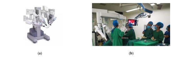
Figure 1.
Pictures showing the Da Vinci robot. (a) The Da Vinci Xi robot, (b) the robot being used for interventional surgery.
A cantilevered articular robot is used when performing interventional puncture to treat prostate cancer. This kind of robotic structure is suitable for human perineal stenosis surgery. However, when the cantilever joint configuration is operated at low velocity and high precision, the changing gravitational torque causes the motor to drive the torque amplitude to fluctuate greatly, and the motor and the robot deteriorates the low velocity motion stability of the robot. Experts and scholars have, thus, been conducting research on robot torque balance [21,22,23].
H. S. Baassan et al. [24] designed a 5-degree-of-freedom flexible hybrid seed implantation mechanism and added a spring with length of 50 mm and stiffness of 0.72 N/mm at the end of the parallel mechanism. The torque generated by the spring was used to balance the heavy torque of the implant. Po-yang Lin et al. [25] studied the elastic balance system of a 3-degree-of-freedom arm, loaded two pull springs onto the connecting rod to balance its own gravity, and solved the appropriate spring stiffness and loading position by establishing a quantitative representation of the maximum stable control stiffness.
However, in addition to the action of the heavy torque, the friction torque generated by the motor and the mechanism during motion is an important factor affecting the stability of the low velocity motion, and there is little research on it.
Therefore, in combination with the above studies, this paper analyzes the influence of the friction torque of robotic joints on motion stability at low velocity. Based on the experimental data of the relationship between velocity and friction torque in the case of no-friction compensation, the velocity point of the minimum torque of the rotating joint and the critical Stribeck velocity point were used as boundary points for segmental parameter identification; cubic spline interpolation was used for segmental fitting equation. Furthermore, the control strategy of the LuGre model is studied: the LuGre model and identification method, parameter identification based on genetic algorithm-particle swarm optimization, and compensation control based on the LuGre friction model. Malab2017a/Simulink was used to simulate and analyze the control strategy to verify its feasibility. Finally, the cantilever prostate seed implantation robot system was tested to verify the effectiveness of the piecewise identification method using the LuGre model and the compensation control strategy based on the genetic algorithm—particle swarm optimization (GA-PSO)—for parameter identification of the LuGre friction model. This model was found to meet the requirements of the cantilever prostate seed implantation robot for position output motion stability at low velocity, providing a vital reference for related research in the field.
2. Structure and Principle
The surgical method of inserting radioactive particles into the prostate is by interventional puncture. During the implantation, the patient is in a supine position with both legs on a leg frame and buttocks at the very end of the bed. This position offers maximize perineum exposure: the legs and torso in the vertical axis are at 90°~100°, the leg bracket clasps the calf muscle, the knee is bent at 90°~100° (parallel to the calf), and the lower limbs are around 80°~90° apart; in this position, the needles are inserted in a horizontal direction.
Therefore, the cantilevered prostate implant robot adopts a horizontal and linear motion, and the axis of the needle is always in a horizontal state. The motion mode of the actuator on the robot positions it as required for the procedure, while the working mode of the robot selects the serial open chain robot, which is composed of a moving pair and two rotating pairs.
The three-dimensional model of the robot is shown in Figure 2. The joint drive motor of the robot with prostate seeds implanted is located on the base, and the axis coincides with the rotation axis of the big arm. Using a parallelogram mechanism, the motion of the motor is transferred to the forearm. In order to keep the actuator horizontal, the implant needle carrier platform is connected to the rotary joint of the big arm using a parallelogram mechanism, where, big arm length is 400 mm, forearm length is 450 mm, and the particle implantation mechanism is 500 mm long.
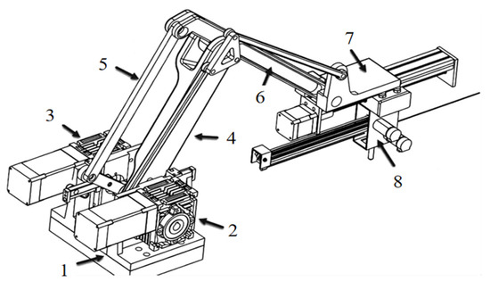
Figure 2.
Structure of the cantilevered prostate seed implantation robot. 1. Base; 2. Joint 1; 3. Joint 2; 4. Big arm; 5. Parallelogram mechanism; 6. Forearm; 7. The implant needle is mounted onto a platform; 8. Seed implantation mechanism.
In order to ensure precision in seed implantation, the fast-tuning robotic arm delivers the implant mechanism to the patient’s perineum near the point of implantation. Then, by fine-tuning the drive joint of the manipulator at low velocity, the seed implantation needle aims precisely at the implantation point. Finally, through the seed implantation mechanism, the seed implantation needle is inserted horizontally into the focal area on the patient’s body. In order to enhance the treatment and reduce trauma, this paper studies the robotic big arm joint and examines its effects with low velocity and high precision regulations. Thus, on combining the clinical experience of urologists at Harbin Medical University with the structure shown in Figure 2, it was found that the tip of the big arm needs to drive forearm movement with linear velocity of 0.01 mm/s–0.05 mm/s. Therefore, the rotational speed of the robotic big arm needs to be adjusted to 0.001°/s–0.007°/s.
It can be seen from Figure 2 that the robot is in a cantilever state when working, and the torque generated by the cantilever dead weight, motor, and joint friction force changes the kinematic characteristics and dynamic performance of the robot at work. Therefore, this paper analyzes the influence of the cantilever prostate implant robot’s motor and the effect of the torque generated by joint friction on low velocity motion control performance.
3. Establishment of a Motor Model and Analysis of Influence of Motion Stability
As the main auxiliary medical device in the treatment of prostate cancer, the cantilever prostate seed implantation robot requires high position accuracy and stability, and its performance has a direct impact on smooth implementation of the surgical treatment. As a key index to evaluate the performance of the robot, the stability of the manipulator at low velocity cannot be ignored.
The accuracy and stability of the cantilever prostate seed implantation robot system is directly affected by the existence of nonlinear factors. When it runs at low velocity, the nonlinearity is more obvious. The oscillations and unsteadiness thus caused will result in steady-state error and affect the tracking accuracy. Therefore, it is necessary to analyze the factors that affect the low velocity performance of the cantilever prostate seed implantation robot. An important factor to be considered is the friction torque caused by motor shaft rotation. Therefore, a mathematical model of its motor system and joint torque needs to first be established, followed by analysis of the influence of friction torque on the stability of the robot’s motion velocity.
3.1. Joint Friction Torque Model of Robot System
When considering the joint friction torque of the cantilever prostate seed implantation robot, the second order nonlinear ordinary differential Equation (1) is generally used [26,27]:
where τf is the nonlinear friction torque of the robot joint; is the action of inertial moment; is the action of coupling moment and centrifugal moment. is gravity torque; τ is the control input torque, τ = rτd, τd is the motor output torque, r is the reduction ratio of the reducer.
In order to identify the friction parameters of the rotating joint friction model, it is necessary to establish a mapping between the friction torque and the joint velocity of the rotating joint at low velocity. Combined with the variable torque compensation device of the robot arm, the gravity of the big arm and forearm of the robot can be compensated in real time, and the impact of load on the friction torque at the robot joints can be ignored [28]; = 0.
If one of the joints in the robot is moved and the other joints are locked, the coriolis force and centrifugal force are 0. Since the big arm and the forearm drive joints of the robot use the same kind of reducer, friction torque at the big arm joints is used for modeling in this paper:
3.2. Motor Model of Robot System
Since the rotating joint of the big arm and forearm of the robot is driven by a DC motor, the voltage and torque balance equation of the servo system can be described as follows:
- Armature voltage balance equation of the DC motor:where is the input voltage of the motor; is the equivalent resistance of the motor armature; is the inductance of the motor; E is the back potential of the motor, , is the angle position.
- Torque balance equation of the brushless DC motor:where is the equivalent moment of inertia of the brushless DC motor; is the velocity of the brushless DC motor; is the total disturbance moment; is the viscosity coefficient, which is generally negligible; is the constant disturbance moment; is the actual torque output of the motor, , is the torque coefficient of the motor; is the armature current; is the torque load generated when the needle is inserted.
Because the low velocity movement of the robot is a precise positioning step outside the body, the load torque generated by the needle relative to the puncture is 0.
After Laplace transform of the above equations, we temporarily set the perturbation moment Mf equal to 0, take the voltage U1 of the brushless dc motor as the input, and the velocity of the brushless dc motor as the output; its transfer function is then expressed as follows:
It can be seen from Equation (6) that the electromagnetic time constant of the motor Te = L/R, and the mechanical time constant of the motor Tm = JR/KmKe. Therefore, Equation (6) can be decomposed into two inertial links, as shown in Equation (7):
When the robot operates at low velocity, Te is generally much smaller than Tm, and the system mainly works in a frequency segment that has low bandwidth at low velocity. Thus, we can ignore the effect of L. Therefore, Equation (7) can be further simplified to Equation (8):
3.3. Effect of Friction Torque on Motion Stability of Robot Joints at Low Velocity
The robot moves due to static friction force on the rotating joint, DC motor, and reducer. During motion, the static friction force is always greater than the dynamic friction force, creating a large imbalance angle. When the rotating joint of the robot moves, the static friction force becomes the dynamic friction force, and the friction force gradually decreases. However, due to the inertia of the system itself, the robotic joint increases its rotation, making the misalignment angle smaller and decreasing the motor torque. As a result, the rotating joint begins to decelerate. When the rotating velocity advances towards 0, the friction force of the rotating joint, the DC motor, and the reducer is transformed into static friction force. The friction torque instantly increases, forcing the mechanical arm to stop rotating. However, as the instructions to move continue, the imbalance angle continues to increase. In order to overcome the static friction force, the output torque of the motor increases again, and the rotating joint re-enters a rotational state. Because this is constantly repeated, it results in what is called the “shake with crawl” phenomenon.
4. Research on Control Methods Based on the LuGre Friction Model
PID is commonly used as a control method for medical robots [29]. When the robot joint runs at low velocity, its velocity control has an obvious nonlinear form, which leads to the generation of phenomena of creep and instability, subsequently affecting low velocity motion performance. Therefore, it is not enough to linearize control with the PID. Among other nonlinear factors, friction torque is the most important factor affecting motion stability of the robot at low velocity. Therefore, it is necessary to design a control strategy to analyze and study the instability caused by friction torque, so as to ensure that the robot runs smoothly at low velocity.
4.1. LuGre Model and Parameter Identification Method
4.1.1. Establishment of the LuGre Model
When compared to other control methods, the friction model-based compensation control method is more specific and effective for friction compensation control of robotic joints at low velocity. According to one study, when compared to other friction models, the LuGre friction model can reflect pre-slip displacement, Stribeck effect, hysteresis, etc.; it is a relatively complete friction model and can accurately describe friction characteristics [30,31,32]. Therefore, the LuGre friction model is adopted in this paper, and its mathematical expression is given as follows:
where is the stiffness coefficient of bristles; is the setae damping coefficient; is the coefficient of viscous friction; is the average amount of deformation of the bristles; describes the Stribeck effect; is coulomb friction; is the maximum static friction force; is Stribeck velocity.
At constant low velocity, the friction torque of the rotating joint of the robot under steady state is expressed as:
where function represents the Stribeck curve of angular velocity and friction torque; the section describes the Stribeck effect.
Critical Stribeck velocity is generally very small, but the value varies from device to device. In the cantilever prostate seed implantation robot used in this paper, critical Stribeck velocity of the big arm joint was measured at 1.2°/s. When the rotating joint of the robot moves at high velocity, its friction torque can be simplified as:
According to Equation (11), when the robot joint is running at high velocity, friction torque is mainly manifested as a combination of Coulomb friction torque and viscous friction torque. The friction torque has no mutation; therefore, it has little impact on the system. However, when the robot joint is running at low velocity, the Stribeck effect cannot be ignored. In such a situation, the friction torque shows strong nonlinearity and has a significant impact on the system.
4.1.2. Parameter Identification Method
After establishing the friction model, parameter identification is important for subsequent friction compensation control. The LuGre friction model needs to identify a total of six parameters, four of which are static, including Coulomb friction torque, maximum static friction torque, viscous friction coefficient, and Stribeck velocity. Two are dynamic parameters, namely, stiffness coefficient of bristles and damping coefficient of bristles.
A two-step identification method is often used to identify the parameters of the LuGre friction model. Static parameters are identified first. The accuracy of the friction model mainly depends on static parameter identification. First, an open-loop system was constructed to allow the revolute joint to run uniformly at different velocities. At this point, the driving force was equal to the friction force. The velocity value and corresponding friction torque value were recorded. Then, a curve fitting method was used to fit the Stribeck curve and identify the static parameters. Finally, the dynamic parameters were identified based on the static parameters.
4.2. Parameter Identification Based on Genetic Algorithm–Particle Swarm Optimization
The LuGre friction model has six parameters. Four Stribeck static parameters need to be identified by intelligent algorithms; however, most researchers mainly use genetic algorithms or particle swarm optimization algorithms. Because these two algorithms are prone to premature or local extremum in the process of seeking an optimal solution, their accuracy in identifying parameters is affected. In order to overcome their shortcomings, in this paper, genetic algorithm–particle swarm optimization (GA-PSO) [33,34] is used for static parameter identification. Based on identification of the static parameters, the local linearization method was used to estimate the dynamic parameters of the LuGre friction model.
4.2.1. The Flow of GA-PSO
- The particle swarm was initialized to determine the population range and position of each particle xi and velocity vi.
- Set the population size of the genetic algorithm (GA), determine the crossover probability, mutation probability, maximum iteration times, etc.
- A genetic algorithm is used to encode the initial value of the particle swarm.
- The coded genetic operators are selected, crossed, and mutated.
- Decodes, calculates fitness values, and adjusts them.
- If iteration times are met, the fitness value is output; if not, step (3) is returned.
- Particle swarm optimization (PSO) was used to compare the individual extremum according to the fitness value obtained by (5). If it is found to be better than the individual extremum, it is identified as the current global optimal position.
- The global extremum is compared according to the fitness value obtained by (5). If it is found to be better than the global extremum, it is identified as the current optimal position and the optimal solution is selected.
- If the termination condition is met, the optimal parameter is output; if the termination condition is not met, proceed to (10).
- As per updates on particle swarm velocity and position, the positions of particle xi and velocity vi are optimized to generate new population particles.
- Return (3).
4.2.2. Static Parameter Identification
The static parameter identification of the LuGre friction model is essentially parameter identification of the Stribeck model, because the latter is a steady-state model. In this paper, identification of the static parameters of the LuGre friction model is based on measured experimental data. The cantilever beam prostate seed implantation robot developed by the Institute of Intelligent Robotics at Harbin University of Science and Technology was tested and analyzed, as shown in Figure 3a.
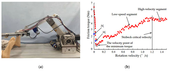
Figure 3.
Diagram of the machine structure and test data. (a) Cantilevered prostate seed implantation robot, (b) experimental data diagram of friction torque and rotation rate.
The big arm joint of the robot was taken as an example for the analysis. According to the surgical velocity requirements of the cantilevered prostate seed implantation robot, the joint was moved at constant velocity within the rotation velocity range of (0~1.5)°/s, and the value of friction torque at different velocities was recorded.
Identification range of static parameters: Fc ∈ [0, 10], Fs ∈ [0, 10], ∈ [0, 1.0], ∈ [0, 10].
Thirty values of torques were recorded at the same velocity, and their average values taken. A total of 92 sets of torques were measured. Figure 3b shows the relationship between friction torque and rotation velocity in the big arm joint system of the robot. The two blue points M1 and M2 in the figure represent—in the process of deceleration regulation—velocity that is less than that at the minimum torque and the value of the friction torque at such a velocity, respectively. In order to obtain accurate static parameters of the LuGre friction model, the measured experimental data is first fitted with a cubic spline interpolation curve [35]. The identification model is then established by comparing the obtained polynomial equation of angular velocity-friction torque with the equations represented by Equations (10) and (11). Finally, (GA-PSO) is used to identify Stribeck parameters so as to obtain the static parameters of the LuGre friction model.
As can be seen from Figure 3b, the critical Stribeck velocity of the cantilevered prostate seed implantation into the big arm of the robot was about 1.2°/s, and when the joint velocity exceeded the critical Stribeck velocity, the friction effect became stable. Therefore, according to Equations (10) and (11), static parameter identification of the LuGre friction model can be divided into a low velocity segment and a high velocity segment, in which the former has the lowest torque when velocity is about 0.05°/s. Most researchers mainly identify a group of results from the low and high velocity segments as a whole [36,37,38,39,40]. However, the friction torque shows a nonlinear trend in moving from low to high velocity segments; thus, tracking precision of the friction torque is difficult to guarantee.
In the velocity point region of the lowest friction torque, and when the rotating joint undergoes repeated acceleration and deceleration fine-tuning, the variation in maximum static friction torque is inconsistent, the main reasons for this being as follows:
- When the rotating joint moves from rest to start, the system has a static friction torque and a large torque of rotational inertia.
- When the rotating joint moves from motion to rest, the system has a dynamic friction torque and a small torque of rotational inertia. This value is much smaller than that of the friction torque at startup.
As a result, in the preoperative preparation stage, friction torque interference is formed in a large area near the point of velocity at the minimum torque during the calibration adjustment, thus affecting positioning accuracy.
Therefore, according to the experimental results, this paper proposes a segmented parameter identification method. The fitting equation is divided into three parts with minimum velocity point of torque and critical Stribeck velocity point as boundary points. In order to ensure continuity of the equation as a whole, in the low velocity segment section, two methods are adopted, acceleration and deceleration. The cubic spline interpolation curve is used to fit them, and the two equations are tangent to each other at the velocity point of the minimum torque; the values of the two equations are equal here. The piecewise equation for low to high velocity is fitted with the cubic spline interpolation curve based on the end parameters of the upper segment as the starting parameters. The fitting results are shown in Figure 4.
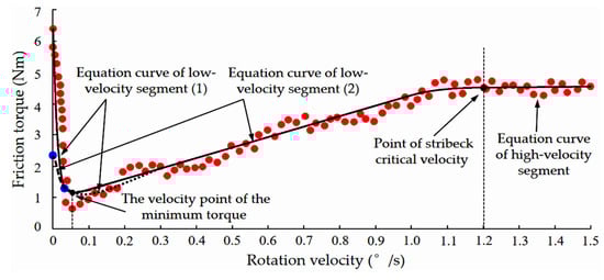
Figure 4.
Fitting diagram of the cubic spline difference curve.
The whole fitting curve equation consists of three parts: Equation curve of the low velocity segment (1) and (2), and equation curve of the high velocity segment (3).
According to the results of the fitting equation shown in Figure 4, and using the curve function toolbox cftool in Matlab-2017a, the “Sum of Sin” function was constructed for the three groups of cubic spline interpolation curves. Three linear equations of friction torque changing with the rotation velocity of the ring motion joint are obtained. The general formula MT is as follows:
where, when ∈ [0°/s, 0.05°/s], MT represents the equation of the low velocity segment (1); ∈ [0.05°/s, 1.2°/s], MT represents the equation of the low velocity segment (2); > 1.2°/s, MT represents the equation of low velocity segment (3); ai, bi and ci represents coefficient of equations, i ∈ [1,4], and i represents the number of terms in the equation.
The identification model is then constructed according to Equation (12), Equation (10), and Equation (11).
4.2.3. GA-PSO Recognition Algorithm Design
Ga-PSO is a hybrid of GA and PSO. The formation of this algorithm is as per the following steps:
- Step 1:
- Setting up of basic parameters
- Selection of parameters in the PSO algorithmPopulation size particle number is 100, population range of each parameter is set according to the range given in Section 4.2.2, dimension is 4, inertia weight is w = 0.62, learning factors c1 = 2, c2 = 2, and the number of iterations is 100.
- Selection of Ga parametersThe population size is 20, individual length is 10, crossover probability Pc = 0.9, variation probability Pm = 0.005, and the number of iterations is 20.
- Step 2:
- Fitness value calculation
- Identification error
- Select the target functionThen, the fitness function is established as per the identification model:
- Step 3:
- Updating the formula of PSO algorithm’s position and velocity:where r1 and r2 are mutually independent random numbers, and the range of variation is between 0 and 1; pis is the individual extreme value; pgs is the global extreme value; xis represents the current position of the particle; vis represents the current velocity of the particle.
The static parameter identification of the LuGre model was carried out according to the flow of GA-PSO as described in Section 4.2.1.
4.2.4. Process and Results of Parameter Identification
In order to verify the effectiveness of GA-PSO identification, the low-speed segment (1) in the MT Equation (12) was chosen for identification. PSO and GA-PSO were used for comparative analysis. Figure 5a,b are fitness curves of PSO and GA, respectively.
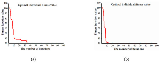
Figure 5.
Comparison and analysis curve of fitness function value. (a) PSO curve, (b) GA-PSO curve.
As shown in Figure 5b, after 100 identification operations, the number of iterations of the GA-PSO converges at (10–13) times, and its adaptive value finally tends to be stable at 30. As can be seen from the comparison between Figure 5a,b, the convergence velocity of PSO is significantly slower than that of GA-PSO. Therefore, GA-PSO is adopted for static parameter identification, which preserves not only the search velocity of PSO, but also the diversity of GA, and improves the overall search ability and accuracy of parameter optimization.
Then, the low velocity segment (2) and high velocity segment (3) in the MT Equation (12) are compared with Equations (10) and (11). The fitness function and identification model were established, and GA-PSO used for identification. The results of the three-segment identification were combined to obtain the Stribeck identification curve.
As shown in Figure 6, the program was written with Matlab2017a software, the friction model was built on the Simulink module, the sampling time was set to 1 ms, and the results were obtained by identification operation based on the Romberg integral solver. As can be seen from Figure 6, the solid black line is the fitting curve of the test data, and the dotted red line is the Stribeck curve obtained after parameter identification by GA-PSO. The change process of the two curves is basically the same, and the equations of the low and high velocity segments are continuous and stable, which verify the accuracy of parameters identified by GA-PSO.
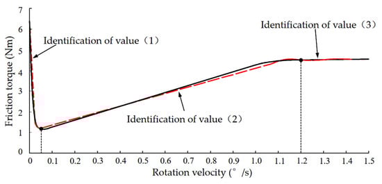
Figure 6.
Results of Stribeck curve parameter identification.
After identification by GA-PSO, three group identification results of the static parameters of the LuGre friction model, corresponding to the three-segment curve equation, are shown in Table 1.

Table 1.
Static parameters of the LuGre friction mode.
4.2.5. Dynamic Parameter Identification
Four static parameters in the LuGre friction model were identified by GA-PSO in Section 4.2.4. Next, only the stiffness coefficient and damping coefficient of the bristles of the two dynamic parameters need to be identified on the basis of the static parameters obtained.
When a small force is applied to the system and it is still in a static state without obvious sliding, the system is said to be in a pre-sliding phase. Equation (9) can be approximately expressed as:
At this point, the system can be approximately regarded as a second-order system, and a tiny step signal is input into the system. When the motion stops:
where: pre-slip displacement; produces the moment of pre-slip displacement . is measured by the torque sensor and by the photocode board.
Then, according to the authors of [41], the damping coefficient of the bristles can be estimated approximately by Equation (18):
where is the equivalent moment of inertia of the system.
The values of and are shown in Table 2.
Table 2.
Dynamic parameters of the LuGre friction model.
Based on the static and dynamic parameters obtained above, an accurate LuGre friction model capable of achieving better friction compensation control can be determined.
4.3. Feedforward Compensation Control Based on the LuGre Friction Model
The so-called compensation control based on the friction model is actually feedforward compensation to the system. The friction force is calculated by a friction model on the basis of certain outputs, and then the estimated friction torque is superimposed on the control torque to reduce friction.
The friction model selected in this paper is the LuGre friction model. Due to the friction state z in the model, specific values cannot be obtained by measurement or calculation. Therefore, a friction state observer must also be designed to estimate friction torque based on the observed state, and then friction compensation control can be carried out by using the controller. According to the mathematical model established in Section 3.1 and Section 3.2, and the LuGre friction model, a basic block diagram of compensation control is established, as shown in Figure 7. In the absence of position control, velocity command is given separately; if given as position signal input, velocity signal input is 0; thus, the velocity command is dotted. Because the implant needle was not inserted into the body when the mechanical arm was adjusted at low velocity, and as it is a process of in vitro regulation, the other interference friction torque was temporarily set to 0.
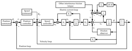
Figure 7.
Diagram of the process of friction torque compensation control.
Based on the control block diagram shown in Figure 7 and the LuGre friction model equation mentioned above, the observer equation is established as follows:
where and are the observed values of and friction torque Mf; is a constant greater than 0.
The observer error:
where ; .
The control law can be obtained by adding the estimation model to the velocity controller:
where J is the equivalent moment of inertia; v is the velocity input signal (v can be expressed as or u1); e is velocity tracking error; is the velocity controller (PID); u2 = H(s)e.
When Equations (4), (21), and (24) are set together, after Laplace transform, the following can be obtained:
If makes strictly regular, state error , friction torque estimation error and velocity error will converge to 0.
According to the above, the friction force obtained by the observer will also gradually converge to the actual friction torque so that the controller can compensate the friction torque in the revolute joint.
5. Simulation Analysis
5.1. Simulation Pre-Experiment
In order to verify the feasibility of the friction compensation control strategy, Matlab2017a/Simulink was used for simulation. If the effect is not ideal, the program can be modified again and the cause of the problem found in time to avoid damage to the experimental equipment. If the effect is satisfactory, it can be safely applied. Previously, experimental data were collected for cantilever beam prostate seed implantation into the arm joint of the robot to identify the static and dynamic parameters of the LuGre friction model. Therefore, this section will take relevant parameters as the research object for simulation and experiment.
In order to prove that there is friction in the movement of the arm joint of the robot when the cantilevered prostate seed implantation robot is fine-tuned (affecting its stability during low-velocity operation), a simulation analysis was done. The framework is shown in Figure 7; the velocity loop and position loop are closed. In a consequent step, a step signal was input with velocity of 0.005°/s, and the angle position curve of the output of the revolute joint system was obtained, as shown in Figure 8.
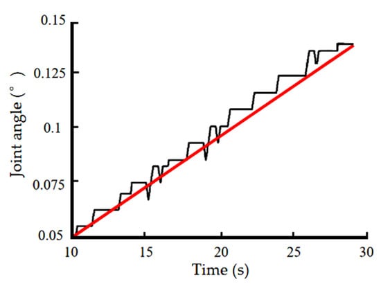
Figure 8.
Angle position tracking curve.
The red line is the theoretical angular position curve, and the black line is the simulation angle position curve. On comparing the theoretical and simulation curves, errors and serious creeping phenomena were found.
As can be seen from the above situation, friction torque has a great impact on the dynamic performance and steady state of the revolute joint. In order to reduce these effects, the friction torque needs to be compensated and controlled. Next, simulation analysis is carried out to verify the effect of friction compensation control.
5.2. PID Control Mode
According to Figure 7, a simulation control frame of PID control of the revolute joint is established and the sine signal of is input into it. The results are shown in Figure 9, where the solid red line is the input curve and the dotted blue line is the output trace curve. As can be seen from Figure 9a, because of friction interference in low velocity rotation, the PID control method has a small deviation in position tracking, and the control effect is not very good. A large position error is shown in Figure 9b; the main cause of this is because when the sinusoidal position signal is in the peak region, its velocity is 0, thus producing large friction torque interference.
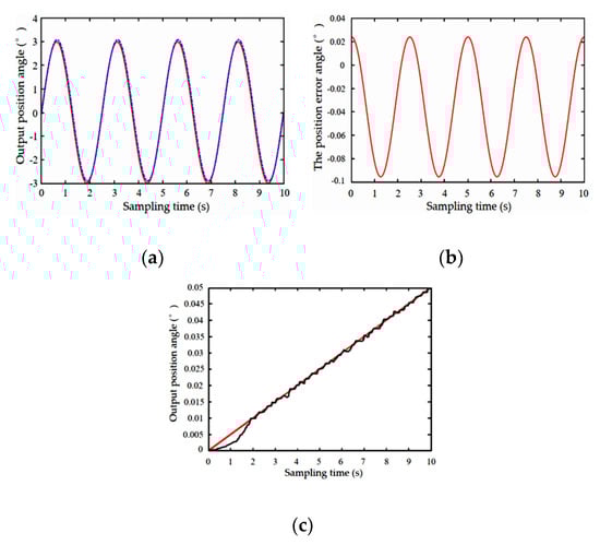
Figure 9.
PID control result. (a) Sin position output for PID control, (b)Position error, (c) PID control angle position output.
At the same time, for step signal with input velocity of 0.005°/s of the simulation model and when the position control is turned off, as shown in Figure 9c, velocity PID control is not ideal. A creeping phenomenon is visible and at the output of the simulation angle position there exists a 2s “dead zone” occurrence. However, when compared with the open-loop control in Figure 8, the effect is found to be a bit better.
The above diagram shows that the PID control effect is not ideal, as it cannot eliminate the crawling phenomenon that arises when the revolute joint is at low velocity, and does not improve its performance.
5.3. LuGre Model Control Mode
On the basis of the PID position control simulation framework, the compensation control strategy of the LuGre model identified by GA-PSO is identified, the segmentation identification method adopted, and the sine signal of input into it. The results in Figure 10a show that the position tracking effect is obviously better than the PID control effect, where the solid red line is the input curve and the dotted blue line is the output trace curve. The position error is shown in Figure 10b. It is obvious that the position error has also greatly decreased, as compared to the PID control.
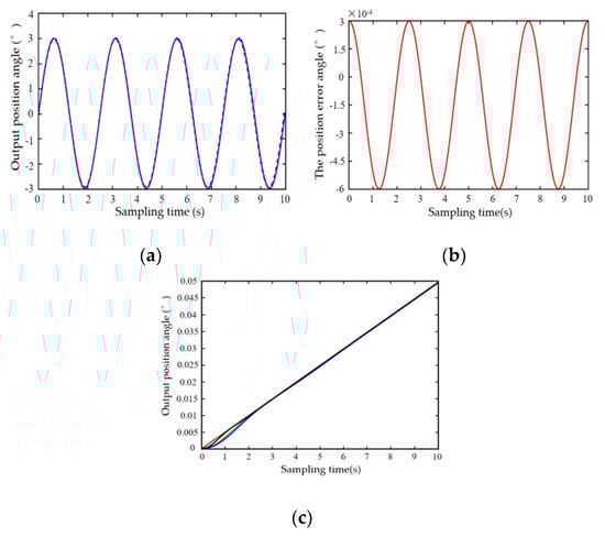
Figure 10.
LuGre model simulation control result. (a) Sin position output under compensated control by the LuGre friction model that offers piecewise parameter identification by GA-PSO; (b) Position error under compensated control by the LuGre friction model that offers piecewise parameter identification by GA-PSO; (c) Angular position output curve under compensated control by the LuGre friction model that offers identification of three kinds of algorithms.
In the step response velocity simulation process, in this paper, PSO, GA, and GA-PSO are used for comparative analysis. The PSO and GA identification LuGre model adopts the whole identification method. Similarly, the step response signal with a velocity of 0.005°/s was input into the simulation model and the position control is turned off. The results are shown in Figure 10c, where the red line represents the theoretical angular position curve with a velocity of 0.005°/s; the blue, green, and black lines represent the simulation angular position curve of the LuGre friction model compensation control identified by PSO, GA, and GA-PSO, respectively.
As can be seen from Figure 10c, the step velocity input-angle position output curve by the LuGre friction model compensation has a good tracking effect and no creeping phenomenon. However, the angle position output controlled by the LuGre friction model identified by PSO and GA still have a 2s “dead zone” phenomenon. On using GA-PSO to identify the LuGre friction model for compensation control, the “dead zone” phenomenon is reduced to less than 1s, and stability of the control is improved.
When compared to the PID control method and the compensation control method based on the LuGre friction model that offers piecewise parameter identification by GA-PSO, the simulation results show that the control method based on the LuGre friction model can reduce the impact of friction torque, eliminate the crawling phenomenon, alleviate the “dead zone” phenomenon in a low velocity state, and improve the low velocity stability of the robot.
6. Results and Discussion
6.1. Control System Introduction and Friction Torque Test Analysis
In Section 4.2.2, a cantilever beam prostate seed implantation robot is introduced; its control system adopts an upper and lower machine structure. Correspondingly, in the test, an upper computer (with a GUI interface made by Matlab2017a) and a lower computer (with an XPC that was compatible with the upper computer’s algorithm program) was used. Hit-pc104-hxl-p515 was used to collect torque and angular position sensor signals for each joint and perform A/D conversion. Hit-pc104-hx l-p520 was used to generate PWM control signals. Each card driver had USES embedded C++ to write s-function modules, as shown in Figure 11a.
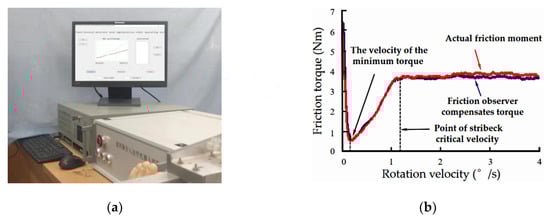
Figure 11.
Diagram of control system and test friction. (a) Diagram of the controller system, (b) Test diagram of the friction torque.
Figure 11b provides a comparison between the actual output friction torque of the revolute joint of the robotic big arm and the friction observer identification friction torque based on the LuGre model that offers piecewise parameter identification by GA-PSO within rotation velocity of (0–4°/s). Here, rotation velocity greater than 1.2°/s is considered high, and the friction torque is nearly stable. It can be seen from the figure that the friction observer identification torque based on the LuGre model can clearly identify the actual friction torque and offset the friction torque to ensure smooth operation of the moving joint at low velocity.
6.2. Comparative Test Between Piecewise Identification Method and Whole Identification Method
In order to verify the effectiveness of the piecewise parameter identification of the LuGre model, the whole and piecewise methods were used to compare and analyze the compensation control process of the model based on fixed parameters. In the experimental process, the GA-PSO method was used to identify the experimental results obtained in Section 4.2.2 by the whole method and segment method, and the identification results obtained, respectively, were used for variable velocity experiment analysis, as shown in Figure 12. The solid blue line and the dotted red line, respectively, represent the theoretical curve and the actual curve of the joint angular position response when the rotation velocity of the arm joint increases from 0 to 1.5°/s at a time of (0–4) s.
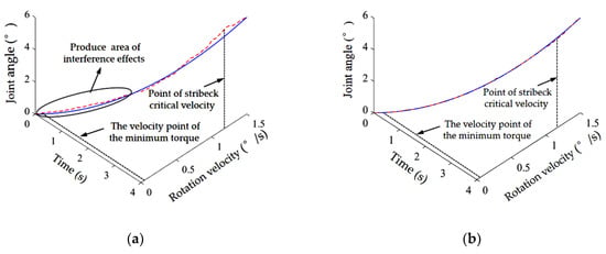
Figure 12.
Comparison of whole identification method and piecewise identification method. (a) Whole identification method, (b) Piecewise identification method.
As can be seen from Figure 12a, the compensation control process of the LuGre friction model based on fixed parameters adopts an overall identification method, and the response curve of the actual angular position is basically consistent with that of a theoretical angular position. However, a bulge change near the velocity point of the minimum torque and the critical Stribeck velocity point is noted, a large area of interference effects is produced, vibrations of the rotating joint with low velocity operation are visible, and dynamic performance of the operation is unstable. Figure 12b is a piecewise identification method for the compensation control process of the LuGre friction model based on fixed parameters. The actual angular position response curve basically coincides with the theoretical angular position response curve, and there is no bulge change near the velocity point of the minimum torque and the critical Stribeck velocity point. The dynamic performance of the rotating joint of the robot is stable at low velocity, which verifies the effectiveness of the piecewise parameter identification of the LuGre friction model.
6.3. Preliminary Work
The main object of this experiment is the big arm joint of a cantilever beam prostate seed implantation robot. For low velocity operation, the performance index requirements are as follows: minimum stationary velocity is 0.005°/s, and error band is ± 0.001°/s. For comparative analysis, conduct four sets of step response signals with input velocity of 0.1°/s, 0.01°/s, 0.005°/s, and 0.001°/s. The four groups of curves in Figure 13 are the angular position curves of the system at different velocity without friction compensation control. The control mode adopts velocity loop (PID) control, position control is turned off, and its angle position is measured by a rotating encoder.
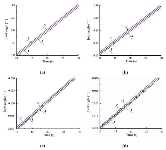
Figure 13.
Angular position curves with different velocity without friction compensation control. (a) angular position curve with a velocity of 0.1°/s; (b) angular position curve with a velocity of 0.1°/s; (c) angular position curve with a velocity of 0.005°/s; (d) angular position curve with a velocity of 0.001°/s.
Figure 13a shows the angular position curve with a velocity of 0.1°/s, from which it can be seen that the system response tracking effect is good with almost no error. Figure 13b shows the angular position curve with a velocity of 0.01°/s. At this point, it can be seen that there is a slight creeping phenomenon during system tracking. Figure 13c is the angular position curve with a velocity of 0.005°/s, at which point the creep phenomenon during system tracking is obvious. Figure 13d is the angular position curve with a velocity of 0.001°/s. These figures clearly show that the crawling and jumping phenomena become more and more obvious as system velocity gradually decreases.
In Figure 13, red line 1 is the theoretical angular position curve, black line 2 is the actual angular position curve, blue line 3 is the error upper boundary curve, and green line 4 is the error lower boundary curve. It can be seen from Figure 11 that the creep phenomenon becomes more and more serious with decrease in velocity, impacting the low velocity performance of the system.
6.4. Comparative Experimental Analysis and Discussion
As per the analysis in Section 6.3, the results in Figure 13c were taken as the reference object in the comparative test. Meanwhile, the system was controlled by the LuGre friction model based on fixed parameters, and the LuGre friction model compensation control strategy to identify parameters by GA and GA-PSO was used for comparative analysis. The results of the low velocity angular position curve of the system after friction compensation control are described below.
Figure 14a shows the actual angular position curve of the system with a velocity of 0.005°/s under compensation control of the LuGre friction model based on GA identification parameters; the parameters of the LuGre friction model were identified by the whole method. It can be seen that the crawling condition is significantly improved, when compared to proportion control. Although the fluctuation of the curve is reduced and the operation is more stable than before, there is some error, indicating that there still exists a large “dead zone” phenomenon. Figure 14b shows the actual angular position curve of the system under the compensation control of the LuGre friction model with a velocity of 0.005°/s based on the identification parameters of GA-PSO; the parameters of the LuGre friction model were identified by the subsection method. The control effect of this method was found to be good, the creep phenomenon was suppressed, and the “dead zone” phenomenon had significantly improved.
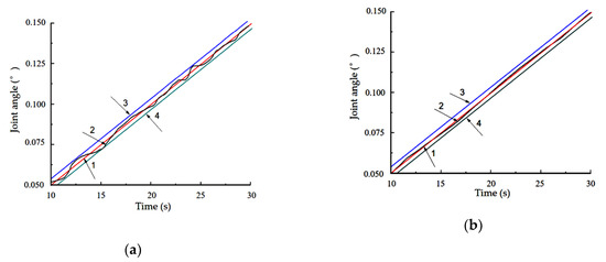
Figure 14.
Comparative analysis. (a) Angular position curve with a velocity of 0.005°/s under LuGre friction model control of identification of whole parameter by GA; (b) angular position curve with a velocity of 0.005°/s under LuGre friction model control of piecewise parameter identification by GA-PSO.
To sum up, the figure shows that with gradual decrease in input velocity rate, the effect of the angular position output of the system became worse. However, with friction compensation control, the effect of the angular position output can improve. The output of the angular position also meets error requirements. In addition, the LuGre friction model is more effective with the piecewise identification method based on GA-PSO. The experiment has reached expected goals and improved the cantilever beam prostate seed implantation robot system’s stability for low velocity motion.
6.5. Position Control Response Comparison Experiment
In order to verify the effect of position tracking, the big arm joint of the robot was used in the experiment. The PID control of the simulation model in Section 5.2 and Section 5.3, and the fixed parameter compensation control of the LuGre friction model based on parameters identified by GA-PSO, were combined for experimental analysis. At the same time, the LuGre friction model adopted a piecewise parameter identification method.
The input sinusoidal signals are shown in Figure 15. The blue dotted line in Figure 15a,c represents the input signal, and the red line represents the tracking signal.

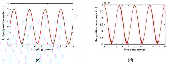
Figure 15.
Result of model control in the course of the experiment. (a) Sin position actual output for PID control; (b) position error; (c) sin position actual output under compensated control by the LuGre friction model with piecewise parameter identification by GA-PSO; (d) position error under compensated control by the LuGre friction model with piecewise parameter identification by GA-PSO.
As can be seen from Figure 15a, the PID control method has deviation in position tracking, and control effect is poor. A large position error is shown in Figure 15b, and the experimental results are consistent with the simulation results. A comparison of Figure 15c and Figure 15d reveals that the LuGre friction model compensation control based on identification parameters of GA-PSO is better than the tracking effect with the PID control alone, verifying the rationality of the simulation analysis.
7. Conclusions
In this paper, the motion output position instability caused by the friction torque of the robot’s motor and rotating joint during low-velocity motion was analyzed and studied. The conclusions are as follows:
On analyzing the main factors affecting low velocity instability, the LuGre model was identified and used to control friction compensation. Experiments were carried out on the big arm joint of the robotic system, and data were obtained to identify the static and dynamic parameters of the LuGre friction model. By comparing PSO and GA, it was found that GA-PSO offered higher convergence speed and optimization accuracy when identifying static parameters of the LuGre friction model, making the identified model more accurate.
In the process of static parameter identification, the minimum velocity point and critical Stribeck velocity point of the friction torque were taken as boundary points. Identification of the cubic spline difference curve fitting parameters were subsequently carried out. By comparing with the whole identification method, the validity and rationality of the method are verified, and dynamic stability of the rotating joint under low velocity operation was found to be improved.
In the sinusoidal position response simulation and PID control simulation, the results show that friction compensation control based on the LuGre friction model is ideal. Meanwhile, PSO, GA, and GA-PSO were used to compare the static parameters that were identified by the LuGre friction model in the simulation of the relationship between velocity and angle position. It was revealed that PSO and GA were able to adopt overall identification, while GA-PSO implemented piecewise identification. Simulation verification discovery was found to effectively alleviate the “dead zone” phenomenon and improve the low velocity stability of the robot.
The LuGre friction model control method (based on GA and GA-PSO for parameter identification) and the PID control method were used to study the relationship between velocity and angle position. The experimental results show that piecewise parameter identification offered by the LuGre friction model based on GA-PSO has a better compensation control effect and effectively inhibits occurrence of the creep phenomenon in low velocity movement of the big arm joint.
A comparative experimental study on the position control response of the big arm joint of the cantilevered prostatic implant robot was carried out. A compensation control method based on the LuGre friction model and the PID control method were used for comparative analysis of sinusoidal position response tracking. The experimental results show that the compensation control method based on the LuGre friction model with piecewise parameter identification by GA-PSO can effectively improve the dynamic performance of rotating joint position tracking for low-speed motion.
In future research, we plan to adopt a new force-bit hybrid tracking control algorithm to study the stability of the robotic rotating joint. This will help ensure the stability of the joint at low velocity and improve its dynamic characteristics, so that doctors can offer prostate cancer patients better, more convenient, and safer treatment options.
Author Contributions
B.L. carried out idea conception, experiment, data analysis, and modification of the article. Y.Z. and L.Y. reviewed and revised the paper. X.X. conducted the experiments and data analysis. All authors have read and agreed to the published version of the manuscript.
Funding
This research is partly supported by the National Natural Science Foundation of China (NSFC), project no. 51675142. Part of the fund was allocated by the key project ZD2018013 at the Natural Science Foundation of Heilongjiang Province, China.
Conflicts of Interest
The authors declare no conflict of interest.
Abbreviation
| GA-PSO | Genetic Algorithm-Particle Swarm Optimization |
| GA | Genetic Algorithm |
| PSO | Particle Swarm Optimization |
References
- Zhang, Y.; Liang, Y.; Wang, X.; Xu, Y. Design and experimental study of joint torque balance mechanism of seed implantation articulated robot. Adv. Mech. Eng. 2015, 7. [Google Scholar] [CrossRef]
- Liao, A.; Wang, J.; Wang, J.; Zhuang, H.; Zhao, Y. Relative biological effectiveness and cell-killing efficacy of continuous low-dose-rate 125i seeds on prostate carcinoma cells in vitro. Integr. Cancer Ther. 2010, 9, 59–65. [Google Scholar] [CrossRef] [PubMed]
- Chen, R.; Sjoberg, D.D.; Huang, Y.; Xie, L.; Zhou, L.; He, D. Prostate specific antigen and prostate cancer in chinese men undergoing initial prostate biopsies compared with western cohorts. J. Urol. 2017, 197, 90–96. [Google Scholar] [CrossRef] [PubMed]
- Zhuo, L.; Cheng, Y.; Pan, Y.; Zong, J.; Zhan, S. Prostate cancer with bone metastasis in Beijing: An observational study of prevalence, hospital visits and treatment costs using data from an administrative claims database. BMJ Open 2019, 9, e028214. [Google Scholar] [CrossRef]
- Zhu, X.D.; Zheng, A.; Wang, Z.Q.; Shao, Q. Prostate cancer prevention trial risk calculator for evaluating the risk of prostate cancer in the high-risk chinese population. Zhonghua Nan Ke Xue/Natl. J. Ofandrol. 2018, 24, 142–146. [Google Scholar]
- Zhu, G.; Zhang, K. Chinese prostate cancer screening: Current situation and challenges. J. Shandong Univ. Health Sci. 2019, 1, 11–15. [Google Scholar]
- Sun, Q.; Sun, S. Diagnostic value of transrectal contrast-enhanced ultrasound -guided biopsy for prostate cancer: A Meta-analysis. J. Clin. Ultrasound Med. 2019, 21, 522–526. [Google Scholar]
- Zhang, L.; Wu, S.; Guo, L.; Zhao, X. Diagnostic strategies and the incidence of prostate cancer: Reasons for the low reported incidence of prostate cancer in China. Asian J. Androl. 2009, 11, 9–13. [Google Scholar] [CrossRef]
- Lin, J.; Yu, X.; Yang, X.; Jin, L.; Zhou, L.; Liu, L.; Su, J.; Li, Y.; Shang, M. High Incidence of Incidental Prostate Cancer in Transurethral Resection of Prostate Specimens in China. The Value of Pathologic Review. Anal. Quant. Cytopathol. Histopathol. 2016, 38, 31–37. [Google Scholar]
- Liang, Y.; Xu, D.; Wang, B.; Zhang, Y.; Xu, Y. Experimental Study of Needle Insertion Strategies of Seed Implantation Articulated Robot. J. Mech. Med. Biol. 2018, 18, 1850023. [Google Scholar] [CrossRef]
- Podder, T.K.; Buzurovic, I.; Huang, K.; Showalter, T.; Dicker, A.P.; Yu, Y. Reliability of EUCLIDIAN: An autonomous robotic system for image-guided prostate brachytherapy. Med. Phys. 2010, 38, 96–106. [Google Scholar] [CrossRef] [PubMed]
- Elayaperumal, S.; Cutkosky, M.R.; Renaud, P.; Daniel, B.L. A passive parallel master-slave mechanism for magnetic resonance imaging-guided interventions. J. Med. Devices 2015, 9, 011008. [Google Scholar] [CrossRef] [PubMed]
- Yu, Y.; Podder, T.; Zhang, Y.; Ng, W.; Misic, V.; Sherman, J. Robotic system for prostate brachytherapy. Comput. Aided Surg. 2007, 12, 366–370. [Google Scholar] [CrossRef] [PubMed]
- Hungr, N.; Troccaz, J.; Zemiti, N.; Tripodi, N. Design of an ultrasound-guided robotic brachytherapy needle-insertion system. In Proceedings of the Annual International Conference of the IEEE Engineering in Medicine and Biology Society, Minneapolis, MN, USA, 3–6 September 2009; pp. 250–253. [Google Scholar]
- Podder, T.K.; Buzurovic, I.; Yu, Y. Multichannel robot for image-guided brachytherapy. In Proceedings of the IEEE International Conference on BioInformatics and BioEnginneering, Philadelphia, PA, USA, 31 May–3 June 2010; pp. 209–213. [Google Scholar]
- Zhang, Z.; Jiang, S.; Sun, F.; Yu, Y. Reliability Analysis of MRI—Guided Surgical Robot for Brachytherapy. In Proceedings of the World Congress on Medical Physics and Biomedical Engineering, Beijing, China, 26–31 May 2013; Volume 39, pp. 2170–2173. [Google Scholar]
- Jiang, S.; Guo, J.; Liu, S.; Liu, J.; Yang, J. Kinematic analysis of a 5-DOF hybrid-driven MR compatible. Robotica 2012, 30, 1147–1156. [Google Scholar] [CrossRef]
- Vaida, C.; Plitea, N.; Gherman, B.; Szilaghyi, A.; Galdau, B.; Cocorean, D.; Covaciu, F.; Pisla, D. Structural analysis and synthesis of parallel robots for brachytherapy. New Trends Med. Serv. Robot. 2014, 16, 191–204. [Google Scholar]
- Zhang, Y.; Liang, Y.; Bi, J.; Xu, Y. Kinematics modeling and simulation of seed implantation robot for prostate tumors. J. Beijing Univ. Aeronaut. Astronaut. 2016, 42, 662–668. [Google Scholar]
- Fu, Y.; Pan, B. Research progress of surgical robot for minimally invasive surgery. J. Harbin Inst. Technol. 2019, 51, 1–15. [Google Scholar]
- Wang, H.; Du, Z.; Yan, Z.; Liu, R. Gravity Compensation Algorithm for Hybrid Master Manipulator. Robot 2014, 36, 111–117. [Google Scholar]
- Diao, Y.; Chen, Z.; Luo, H.; Wu, Y. Minimally invasive surgical robot control based on computing torque. Control Eng. China 2011, 18, 780–782. [Google Scholar]
- Xue, F.; Hou, Z.; Li, X.; Li, N. State switching optimization and global stability control strategy for underactuated two-link manipulator. Chin. J. Sci. Instrum. 2012, 33, 1035–1040. [Google Scholar]
- Bassan, H.S.; Patel, R.V.; Moallem, M. A novel manipulator for percutaneous needle insertion: Design and experimentation. IEEE ASME Trans. Mechatron. 2009, 14, 746–761. [Google Scholar] [CrossRef]
- Lin, P.; Shieh, W.B.; CHEN, D. A theoretical study of weight-balanced mechanisms for design of spring assistive mobile arm support (MAS). Mech. Mach. Theory 2013, 61, 156–167. [Google Scholar] [CrossRef]
- Li, L.; Li, Y.; Zou, Y. Simulation and Experiment of Friction Modeling and Compensation of Scara. J. Syst. Simul. 2019, 31, 1572–1581. [Google Scholar]
- Xi, W.; Chen, B.; Ding, L.; Wu, H.; Xie, B. Dynamic Parameter Identification for Robot Manipulators with Nonlinear Friction Model. Trans. Chin. Soc. Agric. Mach. 2017, 48, 393–399. [Google Scholar]
- Wu, W.; Zhu, S.; Wang, X.; Liu, H. Slow motion control of serial robots with friction compensation based on fuzzy logic system. Electr. Mach. Control 2013, 17, 70–77. [Google Scholar]
- Glozman, D.; Shoham, M. Image-Guided Robotic Flexible Needle Steering. IEEE Trans. Robot. 2007, 23, 459–467. [Google Scholar] [CrossRef]
- Freidovich, L.; Robertsson, A.; Shiriaev, A. LuGre Model Based Friction Compensation. IEEE Trans. Control Syst. Technol. 2010, 18, 194–200. [Google Scholar] [CrossRef]
- Koopman, J.; Jeltsema, D.; Verhaegen, M. Port-Hamiltonian formulation and analysis of the LuGre friction model. In Proceedings of the 47th IEEE Conference on Decision and Control, Cancun, Mexico, 9–11 December 2008; pp. 3181–3186. [Google Scholar]
- Hoshino, D.; Kamamichi, N.; Ishikawa, J. Friction compensation using time variant disturbance observer based on the LuGre model. In Proceedings of the 12th IEEE International Workshop on Advanced Motion Control, Sarajevo, Bosnia-Herzegovina, 25–27 March 2012. [Google Scholar]
- Su, W.; Li, B.; Yan, C.; Zhu, G.; Yuan, L.; Xi, X.; He, J. Force tracking control and test of adaptive hydraulic servo system based on composite particle swarm optimization. J. Northeast Agric. Univ. 2018, 49, 85–96. [Google Scholar]
- Mahmood, A.; Khan, S.; Albalooshi, F.; Awwad, N. Energy-Aware Real-Time Task Scheduling in Multiprocessor Systems Using a Hybrid Genetic Algorithm. Electronics 2017, 6, 40. [Google Scholar] [CrossRef]
- Quan, L.; Shen, J.; Xi, D.; Wang, H.; Liu, L. Motion Planning and Test of Robot for Seedling Tray Handling in Narrow Space. Trans. Chin. Soc. Agric. Mach. 2016, 47, 51–59. [Google Scholar]
- Wu, Y.; Ma, D.; Yao, J.; Le, G. Application of Adaptive Robust Control in Mechatronic Servo System Based on Modified LuGre Model. J. Mech. Eng. 2014, 50, 207–212. [Google Scholar] [CrossRef]
- Zhang, J. Friction Characteristics Identification of Feed System Based on Genetic Algorithm. Agric. Equip. Veh. Eng. 2019, 57, 78–82. [Google Scholar]
- Ma, L.; Wang, J.; Li, F.; Zeng, Y.; Liu, Z. Friction modeling and compensation of precision position system. Guangxue Jingmi Gongcheng Opt. Precis. Eng. 2019, 27, 121–128. [Google Scholar]
- Zhang, W.; Zhao, X.; Tai, X. Parameter identification of gun servo friction model based on the particle swarm algorithm. J. Tsinghua Univ. Sci. Technol. 2007, 47, 1717–1720. [Google Scholar]
- Liu, T.; Wang, H.; Li, Z. Research on Friction Behavior for Direct Feed Drive Based on Intelligent Algorithm. Agric. Equip. Veh. Eng. 2017, 55, 80–83. [Google Scholar]
- Jiang, R.; Liu, C.; Ning, Y. Control Strategy with Adaptive Friction Torque Compensation for Radar Servo System. J. Mech. Eng. 2019, 55, 187–195. [Google Scholar]
© 2020 by the authors. Licensee MDPI, Basel, Switzerland. This article is an open access article distributed under the terms and conditions of the Creative Commons Attribution (CC BY) license (http://creativecommons.org/licenses/by/4.0/).