Article

Design and Implementation of a Digital Dual Orthogonal Outputs Chaotic Oscillator

Institut Jean Lamour (UMR7198) Université de Lorraine, 54011 Nancy, France
*
Author to whom correspondence should be addressed.
Electronics 2020, 9(2), 264; https://doi.org/10.3390/electronics9020264
Submission received: 22 December 2019 / Revised: 23 January 2020 / Accepted: 25 January 2020 / Published: 5 February 2020
(This article belongs to the Special Issue Multidimensional Digital Signal Processing)

Abstract

:
Discrete time dynamical chaotic systems obey a set of recurrence equations involving one or more variables. Many chaotic maps have been proposed. None that simultaneously provides two sine–cosine outputs has stationary mean and standard deviation, or is quite robust with respect to the data format used in the hardware implementation. Here, we propose a chaotic oscillator based on a complex phasor whose angular argument evolves according to a geometric progression that is independent of the instantaneous amplitude. In order to maintain the oscillations, the phasor magnitude is normalized at each iteration using an approximation factor. The statistical characteristics of this oscillator are stationary in the short term, and do not depend on the initial conditions. The mean and standard deviation of the two orthogonal sequences quickly approach 0 and 1 / 2 , respectively. The resulting distribution is similar to that of a digital sine with a constant angular step. We also present an FPGA architecture and its implementation results. This oscillator can be used in modulation schemes, such as the chaotic shift keying one or for data and image encryption. Finally, we show an original application that exploits the orthogonality of the two chaotic signals for the simultaneous encryption of two digital images.

1. Introduction

Chaotic maps offer a mathematical approach that describes the dynamic behavior of systems that are extremely sensitive to the initial conditions. Their study began in the 19th century with the works of Cauchy, Poincaré, Van der Pol and Liapunov. In 1963, Lorenz made a practical use of it for the forecasting of certain meteorological phenomena [1]. In continuous time, they can be represented mathematically by a system of nonlinear differential equations of dimension ≥3. The dynamics of Lorenz, Chen, Rössler and Lu are well-known examples [2]. Discrete time dynamical systems, such as Bernoulli, Hénon and the logistic maps, obey a set of recurrence equations involving one or more variables. More than 100 different chaotic maps have been proposed in the literature.
These systems generate aperiodic signals whose evolution, seen from the outside, lies on the edges between random and deterministic worlds. Therefore, the chaotic oscillators are of major interest for the generation of pseudo-random signals [3,4], or for the encryption of data [5,6,7], speech [8] or images [9,10,11,12]. Various modulation schemes, like the chaos shift keying, use a chaotic carrier in order to secure the transmission and to reinforce its confidentiality [13,14]. Chaotic sequences are also used in compressive sensing to build a measurement matrix that satisfies the restricted isometry property [15,16,17]. In the literature [18], the authors show that a chaotic generator can be used to create a reliable and efficient wireless communication system. Finally, chaotic oscillators and, more generally, systems with nonlinear dynamics, are used to perform complex operations and design stochastic logic systems [19].
Despite their abundance, there is no known chaotic system that simultaneously meets the following criteria:
jointly generates two orthogonal signals, i.e., the outputs are point by point in phase quadrature and constitute a unit vector.
presents statistical characteristics, such as stationary mean and standard deviation, that are also independent of the initial conditions.
is robust when one reduces the sample quantification format.
In an attempt to solve this problem, we looked for systems that implement circular functions that are implicitly normalized. In 1979, Ikeda was one of the first researchers to propose a discrete-time attractor using sine and cosine functions [20]. Then came the chaotic sine map (CSM) and chaotic cosine map (CCM) [21,22]. In order to increase the chaotic complexity, recurrences of the type x k = G [ F ( x k 1 ) ] , where G is a CCM and F a usual chaotic function, were studied more recently [23].
In all of these systems, the instantaneous phase is a function of the previous sample. Here, we propose a chaotic oscillator based on a complex phasor whose angular argument evolves according to a geometric progression that is independent of the instantaneous amplitude.
In the first part of this article, we review the most commonly cited discrete chaotic sequences and highlight their drawbacks, with respect to the three previously mentioned criteria.
The synthesis process and the main properties of the proposed chaotic oscillator are presented in the second part.
The third part analyzes the influence of the quantification on the performance of the oscillator.
Finally, a practical application for fast image cryptography is presented.

2. Usual Digital Chaotic Sequences

2.1. Recurrence Equations

In order to make digital oscillators, one solution is to discretize the differential equations. Numerical differentiation according to the Euler transformation d u ( t ) d t u k u k 1 h is often used. This method requires a sufficiently fine step h, otherwise the sequence generated fades out or diverges very quickly.
One- or multi-dimensional numerical sequences with a more or less pronounced chaotic character according to the internal parameters have also been proposed in the literature. Table 1 provides a synthesis of usual discrete chaotic sequences.

2.2. Influence of the Data Format

Chaotic sequences are very sensitive to the data quantification format. In fact, without special precautions, certain sequences fade very quickly. The Bernoulli map (also named the doubling map in the case of α = 0) vanishes to zero after about 30 or 60 iterates with single precision or double precision floating point computations, respectively. This can be easily demonstrated, as the recurrence relation can be viewed as a left shift operation with the loss of the most significant bit [24].
The Logistic map does not suffer from the vanishing problem with floating point numbers of both single or double precision; but with fixed point representation, there are always cycles in the sequence. The cycles have a duration ranging from a few iterates to a maximum of about 300 iterates for μ = 4, as well as a 2.21 fixed point format.
The sequences obtained by discretized differential equations are also very sensitive to the precision of computations, as well as to rounding rules, which may differ from one processor to another. For example, we show in Figure 1 the evolution over 60,000 points of the signal x k of the Lorenz sequence discretized according to the Euler approximation. The parameters used are σ = 10 , ρ = 28 , β = 8 / 3 , h = 0.001, x 0 = 1 , y 0 = 1 and z 0 = 0.3 . The first computation is carried out by a MATLAB script with the double precision floating point format, using the three recurrence equations provided in Table 1 (Figure 1, left). A second computation is carried out according to the same mathematical approach and with the same computer, but this time we used a Simulink diagram in discrete mode.
According to Figure 2, very strong differences appear from the 45,000th iterate. This dependency creates a problem when such sequences are used, for example, for cryptographic applications.

2.3. Statistical Variability

The statistical characteristics of chaotic sequences such as the mean (m) and standard deviation (std) may depend on the intrinsic parameters and initial conditions. This is particularly true for discretized differential equations. The variations of the latter being slow with respect to h, and the estimates of m and std require a large number of samples. Table 2, for example, shows the high variability of the mean of the discrete Lorenz sequence on 100,000 x k samples.
The Logistic and Hénon sequences have m and std values, independent of the initial conditions. Their values are 0.64 and 0.06, respectively, for the logistic sequence, with μ = 3.8 and 0.26 and 0.72 for the Hénon sequence. Nevertheless, the standard deviation of the logistic suite is strongly influenced by the parameter μ.

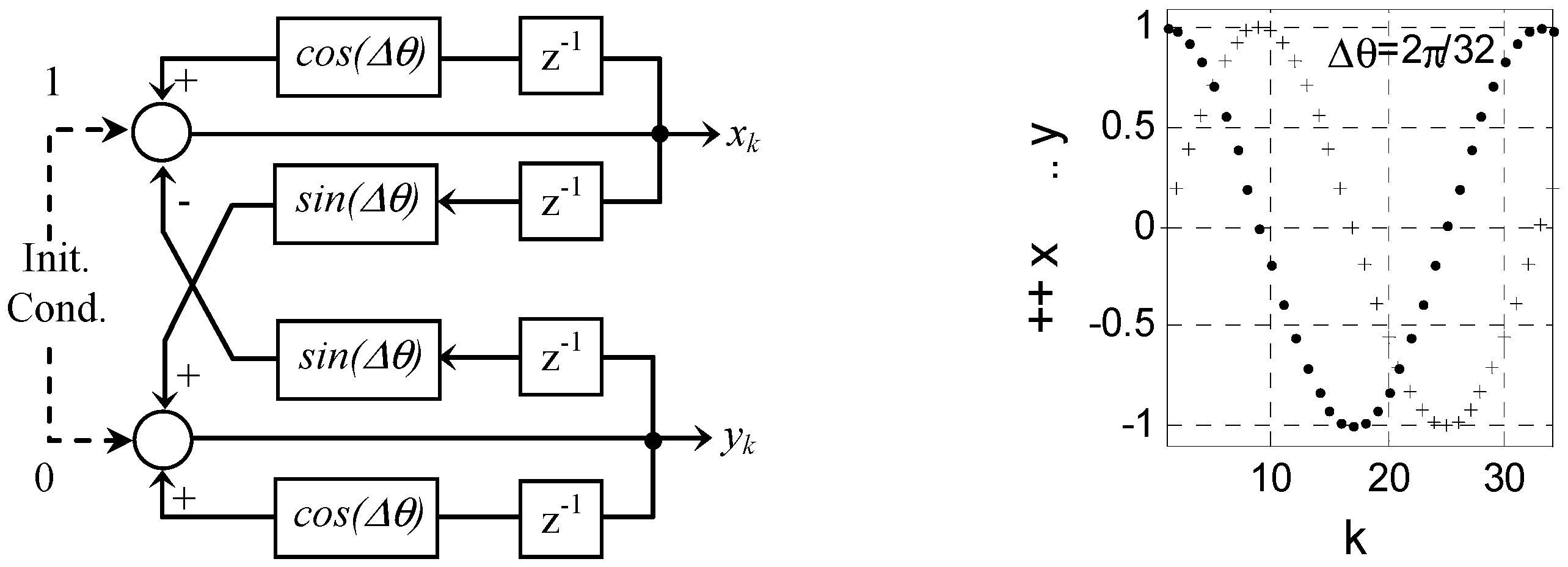
3. Proposed Orthogonal Chaotic Sequence

3.1. Theoretical Background

We consider a digital oscillator that simultaneously generates at time k the outputs xk and yk, given by the following:
x k = c o s ( k Δ θ )   and   y k = s i n ( k Δ θ )
where Δ θ is the angular step and ( x 0 = 1 and y 0 = 1 ) are the initial conditions. Equation (1) corresponds to the complex phasor, as follows:
W k = x k + j y k = e j θ k = e j k Δ θ
The recurrence relation W k = e j Δ θ W k 1 leads to the following:
x k = c o s ( Δ θ ) x k 1 s i n ( Δ θ ) y k 1 y k = s i n ( Δ θ ) x k 1 + c o s ( Δ θ ) y k 1
This oscillator uses the principle of the angular integration depicted in Figure 2.
We consider a phasor whose argument θ k follows a geometric progression with a common ratio of two. It follows the recurrence relations of Equation (4), as follows.
W k = W k 1 2     x k = x k 1 x k 1 y k 1 y k 1 y k = y k 1 x k 1 y k 1 y k 1
This is equivalent to substituting functions y k 1 and y k 1 for coefficients c o s ( Δ θ ) and s i n ( Δ θ ) , respectively, in the previous diagram. If the initial phase θ 0 is exactly equal to 0 or 2 π / 2 N , the system stabilizes itself in the states ( x k = 1 and y k = 0 ) and ( x k = 0 and y k = 1 ).
On the other hand, the oscillator is very sensitive to the initial phase conditions. For example, Figure 3 shows the first 60 samples of x k and y k obtained for the two initial phases separated by a 0.001 rad (computations performed with MATLAB with double precision numbers).

3.2. Normalized Recurrence Equations

In practice, the phase errors due to the quantization accumulate and lead to the fade-out of signals. In order to overcome this problem, it is necessary to ensure that the relation r k 2 = x k 2 + y k 2 = 1 is satisfied at each iteration. This can be achieved by using the normalized Equations (5).
x k = x k 1 2 y k 1 2 x k 1 2 y k 1 2   and   y k = 2 x k 1 y k 1 x k 1 2 + y k 1 2
Equations (5) allow for the use of initial conditions other than the pair ( c o s θ 0 and s i n θ 0 ). The values of x 0 0 and y 0 0 , such as x 0 y 0 , can also ensure the start of the oscillator. The orthogonalization and the normalization of the signals appear by the second iteration.

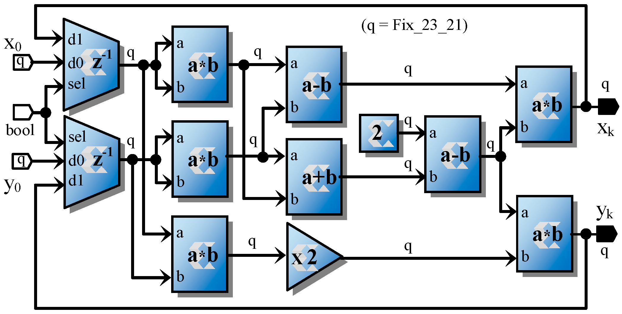
3.3. Approximation of Normalized Recurrence Equations

To eliminate the dividers in Equations (5), the following approximation is used:
x k 1 2 + y k 1 2 1 + ε     1 x k 1 2 + y k 1 2 1 ε 2 ( x k 1 2 + y k 1 2 )
Using this relation, we get the following:
r k 2 = [ ( x k 1 2 y k 1 2 ) 2 + 4 x k 1 2 y k 1 2 ] [ 2 ( x k 1 2 + y k 1 2 ) ] 2 = [ ( x k 1 2 + y k 1 2 ) 2 ] [ 2 ( x k 1 2 + y k 1 2 ) ] 2
Thus,
r k = r k 1 2 ( 2 r k 1 2 )
Finally,
{ x k = ( x k 1 2 y k 1 2 ) ( 2 ( x k 1 2 + y k 1 2 ) ) y k = 2 x k 1 y k 1 ( 2 ( x k 1 2 + y k 1 2 ) )
The asymptotic algorithmic complexity of our map is therefore O(n).
The magnitude of the generated points obeys Equation (8). Its evolution strongly depends on the initial value r 0 . Only a convergence of r k towards 1 makes it possible to maintain a steady chaotic state.
The continuous function f ( w ) = w 2 ( 2 w 2 ) corresponding to Equation (8) has three positive roots, namely, 0, 1 and 1 φ = 5 1 2 = 0.618 , where φ = 1.618 is the golden ratio.
The dynamic behavior of Equation (6) is analyzed by the mean of the function f(w). Values 0 and 1 are attractive points, and 1 / φ is a repulsive point. The main convergence intervals are summarized in Table 3.
In conclusion, the values x 0 = c o s ( θ 0 ) and y 0 = s i n ( θ 0 ) , and more broadly, all the initial values ( x 0 , y 0 ) , whose magnitude corresponds to case number two in Table 3, make it possible to generate a maintained chaotic oscillator.

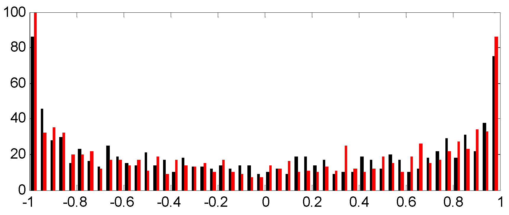
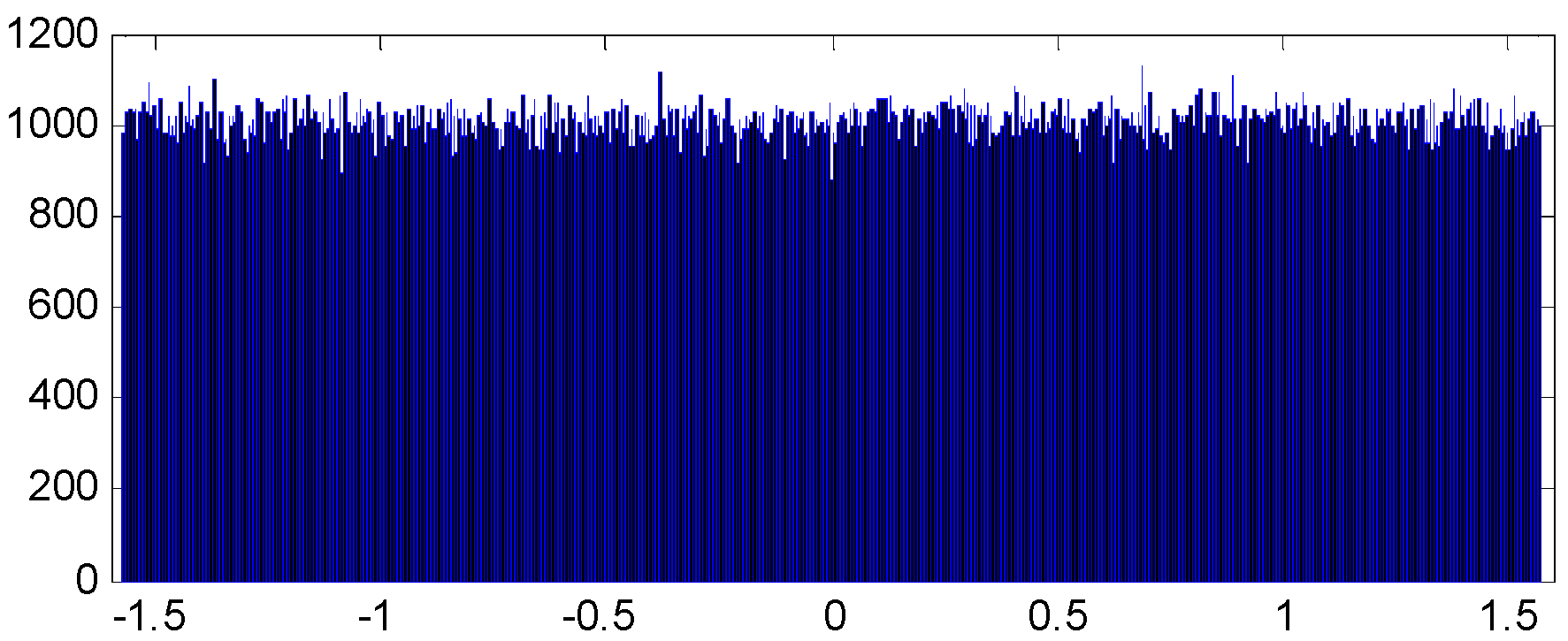
3.4. Statistic Properties of the Chaotic Oscillator

As the proposed oscillator generates sine and cosine functions, its statistical characteristics are stationary in the short term. The mean and standard deviation of the two sequences quickly approach 0 and 1 / 2 , respectively. The trajectories of the oscillator signals in different planes are presented in Figure 4.
where d x = x k x k 1 and d y = y k y k 1 are the differentials of x and y, respectively.
The first two diagrams show butterfly-shaped trajectories. The circular envelope of the (x, y) points is characteristic of quadrature signals.
The observed dynamics are similar to the Ikeda attractor in the (x, y) plane and to the Hénon attractor in the (dx and x) plane.
The histogram on 1000 points of x and y shows a non-uniform distribution of output values (Figure 5). This distribution is similar to that of a digital sine with a constant angular step. On the other hand, the instantaneous angular phase θ k is uniformly distributed between −π and π, as shown in the histogram of Figure 6, made from a million values.

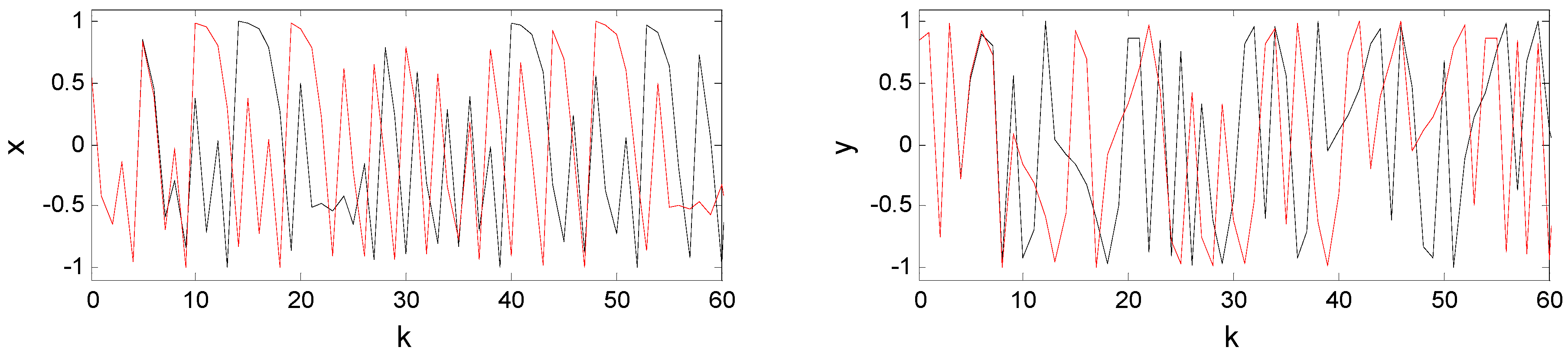
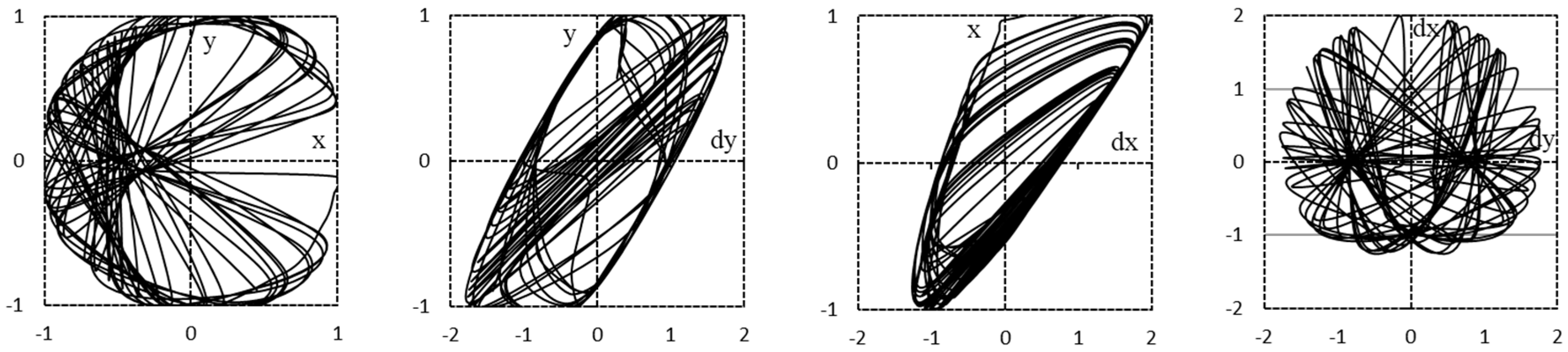
3.5. Chaotic Behavior Analysis

The recognition and quantification of chaos in a digital signal has been the subject of different approaches. Among them, the estimate of Lyapunov’s largest exponent λ of the progression is one of the most reliable. This parameter measures the average exponential rate of divergence or convergence between two trajectories of the sequence resulting from very close initial conditions. Three situations can occur, namely:
λ < 0 corresponds to an orbital trajectory attracted by a stable fixed point. This situation is representative of strongly deterministic, harmonic or random sequences.
λ very close to 0 represents a steady state close to a chaotic transition.
λ > 0 characterizes an unstable and chaotic orbit. The larger λ, the more chaotic character is observed.
In order to study the dynamics of financial markets, A Bensaida developed a neuron network-based chaos test algorithm that mimics the chronological behavior of the sequence to be analyzed [25]. We used this algorithm because it requires no prior knowledge of the signal to be analyzed, and can also be used on noisy data. Table 4 compares the Lyapunov coefficients recorded on the Logistic progression, Hénon sequence and the signals delivered by the proposed oscillator. The estimates are made on 1000 points, with the same configuration of the neural network.
This comparison confirms the chaotic character of the signals x k and y k , with a higher grade of x k .

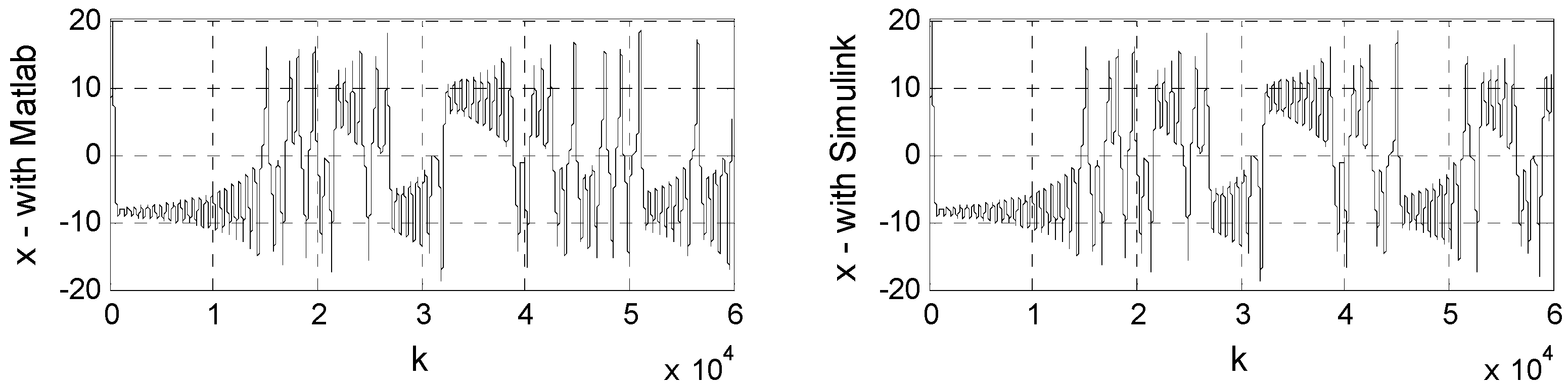
4. Hardware Implementation

The oscillator was also implemented on a Xilinx FPGA target (Zynq UltraScale+ MPSoC ZCU106). The implementation diagram is given in Figure 7.
As the dynamics of x k and y k are limited to the interval [−1; 1], a quantization format with 23 bits, of which 21 are reserved for the fractional part, is sufficient to sustain the oscillations and to provide a reasonably large enough period (more than 2820 iterations), compared to a single precision floating point implementation (more than 1920 iterations). Table 5 summarizes the necessary hardware resources, power consumption and the maximum sampling frequency fs obtained for three different calculation accuracies, namely, double precision floating point (IEEE754 64-bit), single precision floating point (IEEE754 32-bit) and the custom defined fixed-point format, with two bits for the integer part and 21 bits for the fractional part.
In this case, one can see that an algorithm architecture matching the methodology provides a resulting architecture that lowers the necessary hardware resources, consumes less power, has a greater throughput and has a similar or even better accuracy than its direct “translation” from a software model.

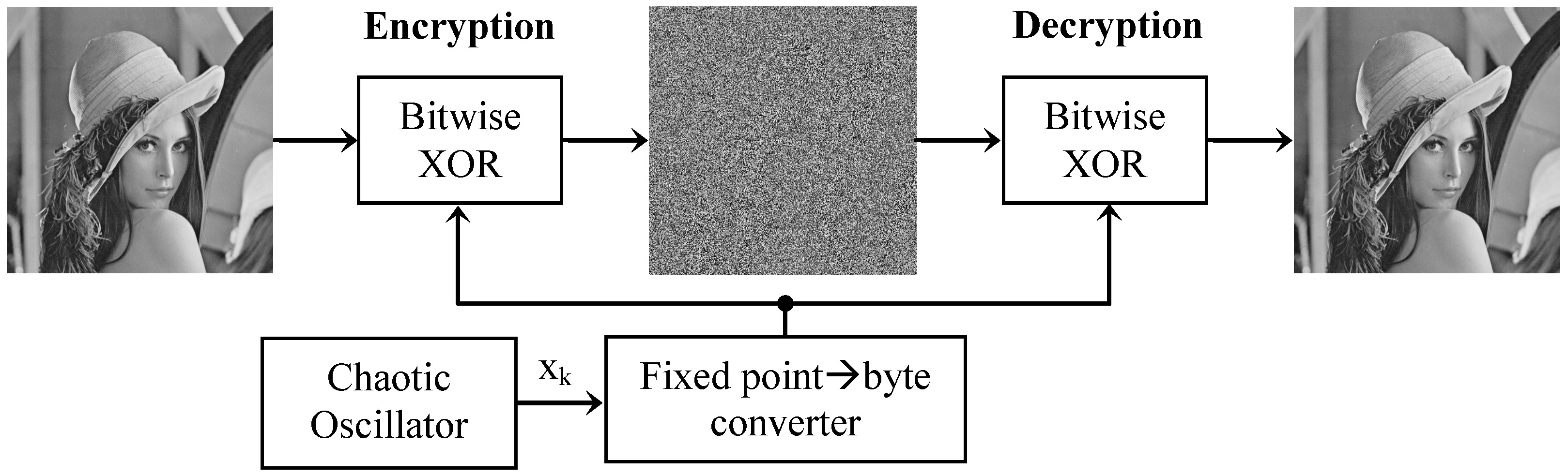
5. Application to the Fast Image Encryption

5.1. Image Encryption/Decryption With Bitwise XOR Operation

Many authors use chaotic systems to encrypt digital images. Basically, the encryption processes of an image plane of N*M pixels remain similar, and take place in three successive stages, namely:
Elaboration of a sequence of N*M numerical coefficients of the chosen chaotic system in which the precise initial conditions have been introduced.
Quantification of the coefficients in a format identical to that of the pixels of the original image (eight bits in most cases). Given the variability of the statistical characteristics of the sequence with the initial conditions, this operation can only be carried out after the computation of the entire sequence.
Application of a bitwise XOR operation between the pixel values and the quantized coefficients.
The decryption of the image is carried out according to the same approach.
The use of this coding strategy with the proposed chaotic system is also possible. In this case, the quantification is easy because of the statistical stability of the sequence. Indeed, the range of our sequence is [−1; 1], therefore it becomes very easy to convert it into, for example, a sequence of eight-bit words. The hardware resources needed are very low, as it only requires a fixed-point increment whose output is truncated to the eight most significant bits. The scheme of this method with the proposed chaotic oscillator is shown in Figure 8.

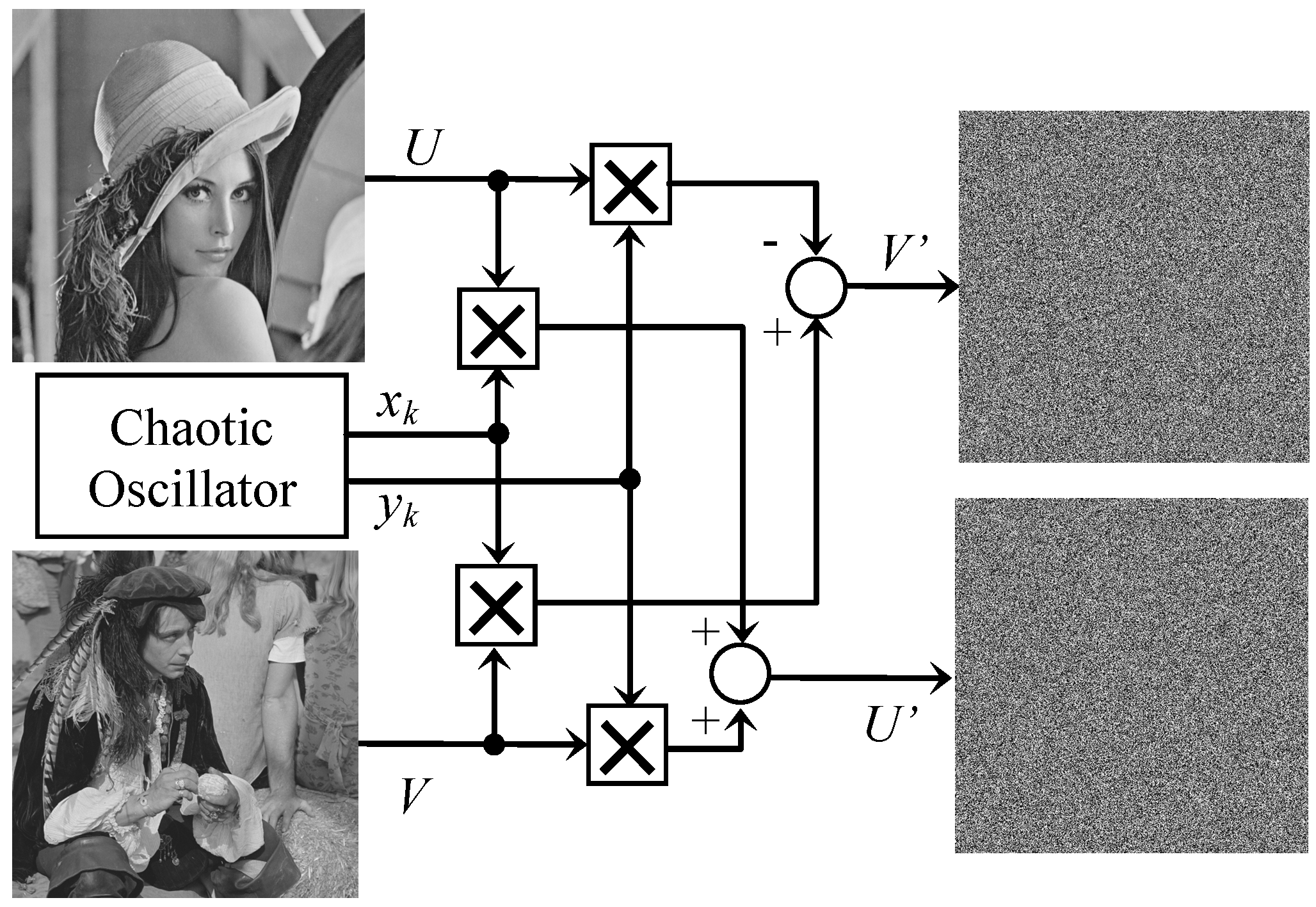
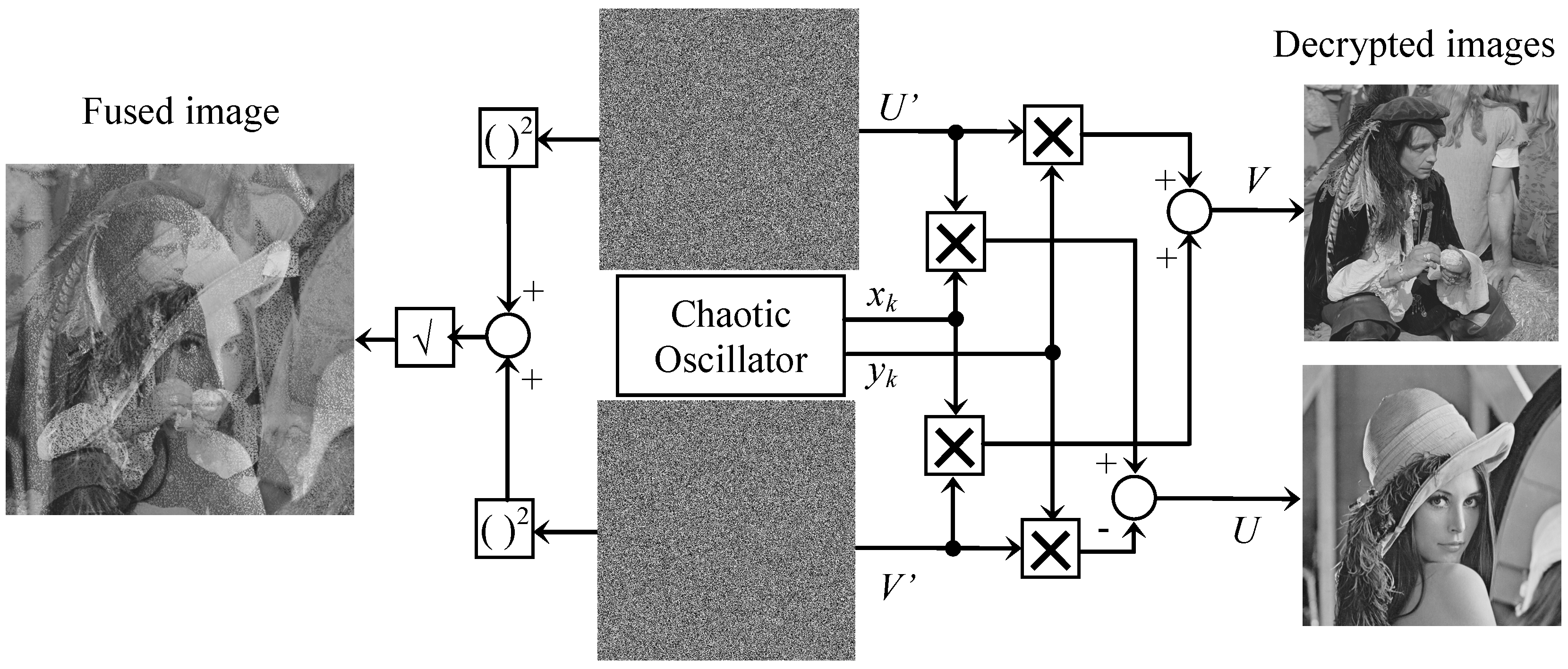
5.2. Simultaneous Images Mixing Encryption/Decryption

We propose a second process, which can be used if the confidentiality of the information is not the main criterion.
Let U and V be two different grayscale images of the same size N*M.
Let k be the position of a pixel in the image, according to the conventional scanning from left to right and from top to bottom.
The u k and v k pixels of each image can be considered as the Cartesian coordinates of a point P ( u k , v k ) , respectively.
Let us apply a rotation of an angle θ k to each point P.
This operation leads to point P ( u k , v k ) , such that:
u k = u k c o s ( θ k ) + v k s i n ( θ k ) v k = u k s i n ( θ k ) + v k c o s ( θ k )     u k = u k x k + v k y k v k = u k y k + v k x k
where the ordered pairs ( x k , y k ) are generated by the orthogonal outputs of the proposed chaotic oscillator.
The values u k and v k provide two encrypted images, named U’ and V’, respectively.
Two uniform images represented by a single point P are located after this transformation in a different point P’, distributed randomly on a circle of the same radius.
The transformation is reversible. It is performed by a reverse rotation, as follows:
u k = u k x k v k y k v k = u k y k + v k x k
This principle is similar to that of a synchronous modulation/demodulation with a random frequency.
The algorithm for the encryption is as follows:
Step 1:
Read the two original images with size N*M, then convert them into one dimensional arrays U and V, and assign the initial conditions x0 and y0.
Step 2:
For each pair (uk and vk), compute the following:
u k = u k x k + v k y k
v k = u k y k + v k x k
x k + 1 = ( x k 2 y k 2 ) ( 2 ( x k 2 + y k 2 ) )
y k + 1 = 2 x k y k ( 2 ( x k 2 + y k 2 ) )
Step 3:
Convert the two arrays U’ and V’ into two images with the size N*M.
The algorithm for the decryption is as follows:
Step 1:
Read the two encrypted images with size N*M, then convert them into one-dimensional arrays U’ and V’, and assign initial conditions x0 and y0.
Step 2:
For each pair (u’k and v’k), compute the following:
u k = u k x k v k y k
v k = u k y k + v k x k
x k + 1 = ( x k 2 y k 2 ) ( 2 ( x k 2 + y k 2 ) )
y k + 1 = 2 x k y k ( 2 ( x k 2 y k 2 ) )
Step 3:
Convert the two arrays of U and V into two images with the size N*M.
The asymptotic algorithm complexity of both the encryption and decryption is O(N*M).
We applied this encryption method using the digital architecture described in the previous paragraph. Figure 9 and Figure 10 illustrate the encryption and decryption, respectively, of the original images (Lena and the Pirate, respectively).
Upon reception, a visualization of the addition of the two images can be carried out very simply by performing the computation u k 2 + v k 2 , which is equal to u k 2 + v k 2 .
However, the separation of the two images cannot be achieved without knowledge of the chaotic sequence.
A practical application of this process is merging pairs of pages from a book in order to provide a quick overview to the reader, who, if interested, can request the decryption key from the publisher.

6. Conclusions

We propose a chaotic oscillator using a complex phasor with phase doubling at each sampling time. The recursive structure performs the angular integration and simultaneously generates two orthogonal signals representative of the pair (cosine and sine). The nonlinear evolution of the phase is responsible for the chaotic behavior that we confirmed by the positive Lyapunov coefficients evaluated on the generated signals.
Thanks to the trigonometric properties related to the double angle, no direct computation of the cosine and sine functions is necessary.
The permanence of the oscillations is obtained using a normalization of the magnitude of the ordered pairs ( x k and y k ) carried out at each iteration.
In order to simplify the implementation of the system, the normalization ratio is replaced by an approximation factor. The recurrence equations thus take a purely polynomial form.
The analysis of the dynamics of the system shows that any initial pair ( x 0 and y 0 ) whose magnitude is between 0.618 and 1.272 ensures a chaotic behavior.
The hardware implementation of this oscillator is presented and the influence of the quantification format on the chaotic complexity is studied. A fixed point 23-bit format, including 21 bits for the fractional part, allows for the generation of deterministic chaos with a periodicity greater than 2800.
This oscillator can be used in modulation schemes, such as the chaotic shift keying one and for data and image encryption. We finally show an original application that exploits the orthogonality of the two chaotic signals for the simultaneous encryption of two digital images.

Author Contributions

Conceptualization and methodology, Y.B. and E.T.; software, Y.B. and E.T.; FPGA implementation, H.R., validation, Y.B., E.T., P.P. and H.R.; writing—original draft preparation, Y.B., E.T. and P.P.; writing—review and editing, P.P. All authors have read and agreed to the published version of the manuscript.

Funding

This research received no external funding.

Conflicts of Interest

The authors declare no conflict of interest.

References

  1. Lorenz, E.N. Deterministic nonperiodic flow. J. Atmos. Sci. 1963, 20, 130–141. [Google Scholar] [CrossRef] [Green Version]
  2. Leonov, G.; Kuznetsov, N. On differences and similarities in the analysis of Lorenz, Chen, and Lu systems. Appl. Math. Comput. 2015, 256, 334–343. [Google Scholar] [CrossRef] [Green Version]
  3. Koyuncu, I.; Özcerit, A.T.; Pehlivan, I. Implementation of FPGA-based real time novel chaotic oscillator. Nonlinear Dyn. 2014, 77, 49–59. [Google Scholar] [CrossRef]
  4. Sambas, A.; Vaidyanathan, S.; Tlelo-Cuautle, E.; Zhang, S.; Guillen-Fernandez, O.; Hidayat, Y.; Gundara, G. A Novel Chaotic System with Two Circles of Equilibrium Points: Multistability, Electronic Circuit and FPGA Realization. Electronics 2019, 8, 1211. [Google Scholar] [CrossRef] [Green Version]
  5. Chen, S.L.; Hwang, T.; Chang, S.M.; Lin, W.W. A fast digital chaotic generator for secure communication. Int. J. Bifurcation Chaos 2019, 20, 3969–3987. [Google Scholar] [CrossRef]
  6. Liao, T.-L.; Wan, P.-Y.; Chien, P.-C.; Liao, Y.-C.; Wang, L.-K.; Yan, J.-J. Design of High-Security USB Flash Drives Based on Chaos Authentication. Electronics 2018, 7, 82. [Google Scholar] [CrossRef] [Green Version]
  7. Li, W.; Wang, C.; Feng, K.; Huang, X.; Ding, Q. A multidimensional discrete digital chaotic encryption system. Int. J. Distrib. Sens. Netw. 2018, 14, 1–8. [Google Scholar] [CrossRef]
  8. Alroubaie, Z.M.; Hashem, M.A.; Hasan, F.S. FPGA Design of Encryption Speech system using Synchronized Fixed-Point Chaotic Maps Based Stream Ciphers. Int. J. Eng. Adv. Technol. 2019, 8, 2249–8958. [Google Scholar]
  9. Zhang, W.; Zhu, Z.; Yu, H. A Symmetric Image Encryption Algorithm Based on a Coupled Logistic–Bernoulli Map and Cellular Automata Diffusion Strategy. Entropy 2019, 21, 504. [Google Scholar] [CrossRef] [Green Version]
  10. Liu, H.; Kadir, A.; Sun, X. Chaos-based fast colour image encryption scheme with true random number keys from environmental noise. IET Image Process. 2017, 11, 324–332. [Google Scholar] [CrossRef]
  11. Zhang, Q.; Guo, Y.; Li, W.; Ding, Q. Image encryption method based on discrete lorenz chaotic sequences. J. Inf. Hiding Multimed. Signal Process. 2016, 7, 575–586. [Google Scholar]
  12. Rohith, S.; Bhat, K.H.; Sharma, A.N. Image encryption and decryption using chaotic key sequence generated by sequence of logistic map and sequence of states of Linear Feedback Shift Register. In Proceedings of the 2014 International Conference on Advances in Electronics Computers and Communications, Bangalore, India, 10–11 October 2014; pp. 1–6. [Google Scholar]
  13. Kennedy, M.P.; Kolumbán, G.; Kis, G. Chaotic Modulation for Robust Digital Communications over Multipath Channels. Int. J. Bifurc. Chaos 2000, 10, 695–718. [Google Scholar] [CrossRef]
  14. Babu, S.B.S.; Kumar, R. 1D-Bernoulli Chaos Sequences Based Collaborative-CDMA: A Novel Secure High Capacity CDMA Scheme. Wirel. Pers. Commun. 2017, 96, 2077–2086. [Google Scholar] [CrossRef]
  15. Liu, L.; Yang, P.; Zhang, J.; Ja, H. Compressive sensing with Tent chaotic sequence. Sensors Transducers 2014, 165, 119–124. [Google Scholar]
  16. Yu, L.; Barbot, J.P.; Zheng, G.; Sun, H. Compressive Sensing With Chaotic Sequence. IEEE Signal Process. Lett. 2010, 17, 731–734. [Google Scholar]
  17. Linh-Trung, N.; Minh-Chinh, T.; Tran-Duc, T.; Le, H.V.; Do, M.N. Chaotic compressed sensing and its application to magnetic resonance imaging. J. Electron. Commun. 2013, 3, 84–92. [Google Scholar] [CrossRef]
  18. Ren, H.-P.; Bai, C.; Liu, J.; Baptista, M.S.; Grebogi, C. Experimental validation of wireless communication with chaos. Chaos: Interdiscip. J. Nonlinear Sci. 2016, 26, 083117. [Google Scholar] [CrossRef] [Green Version]
  19. Venkatesh, P.R.; Venkatesan, A.; Lakshmanan, M.; Ramadass, V.P. Implementation of dynamic dual input multiple output logic gate via resonance in globally coupled Duffing oscillators. Chaos: Interdiscip. J. Nonlinear Sci. 2017, 27, 083106. [Google Scholar] [CrossRef]
  20. Ikeda, K. Multiple-valued stationary state and its instability of the transmitted light by a ring cavity system. Opt. Commun. 1979, 30, 257–261. [Google Scholar] [CrossRef]
  21. Zhu, S.; Wang, G.; Zhu, C. A Secure and Fast Image Encryption Scheme based on Double Chaotic S-Boxes. Entropy 2019, 21, 790. [Google Scholar] [CrossRef] [Green Version]
  22. Ogras, H.; Turk, M. A secure chaos-based image cryptosystem with an improved sine key generator. Am. J. Signal Process. 2016, 6, 67–76. [Google Scholar]
  23. Alawida, M.; Samsudin, A.; Teh, J.S.; AlShoura, W.H. Digital Cosine Chaotic Map for Cryptographic Applications. IEEE Access 2019, 7, 150609–150622. [Google Scholar] [CrossRef]
  24. Rochberg, R. The equation (i-s)g = f for shift operators in Hilbert space. Proc. Am. Math. Soc. 1968, 19, 123–129. [Google Scholar]
  25. Ben Saïda, A. Noisy chaos in intraday financial data: Evidence from the American index. Appl. Math. Comput. 2014, 226, 258–265. [Google Scholar]
Figure 1. Lorenz sequence computed with MATLAB (left) and Simulink (right).
Electronics 09 00264 g001
Figure 2. Block diagram and signals of a digital sine–cosine oscillator.
Electronics 09 00264 g002
Figure 3. Oscillator outputs for very close initial conditions ( θ 0 = 0.999 in black and θ 0 = 1.0 in red).
Electronics 09 00264 g003
Figure 4. Signals trajectories in different planes.
Electronics 09 00264 g004
Figure 5. Histogram of x (black) and y (red).
Electronics 09 00264 g005
Figure 6. Histogram of the phase θ.
Electronics 09 00264 g006
Figure 7. FPGA implementation diagram of the chaotic digital oscillator.
Electronics 09 00264 g007
Figure 8. Image encryption/decryption with a bitwise XOR operation.
Electronics 09 00264 g008
Figure 9. Simultaneous encryption of two images.
Electronics 09 00264 g009
Figure 10. Degraded view and decryption of the two images.
Electronics 09 00264 g010
Table 1. Usual chaotic numerical time series.
Dim.ModelRecursive EquationsChaos Conditions
1DLogistic x k = μ x k 1 ( 1 x k 1 ) x 0 ] 0 ,   1 [
3.57 μ < 4
1DBernoulli x k = 2 1 α ( x k 1 + 1 ) 1   1 < x k 1 < α
x k = 2 1 α ( x k 1 1 ) + 1 α < x k 1 < 1
1 < α < 1
2DHénon x k = y k 1 + 1 a x k 1 2
y k = b x k 1
a = 1.4
b = 0.3
3DLorenz discrete
(Euler approx.
dt = h)
x k = x k 1 σ h ( x k 1 y k 1 )
y k = y k 1 + h ( ρ x k 1 y k 1 x k 1 z k 1 )
z k = z k 1 + h ( x k 1 z k 1 β z k 1 )
σ = 10 ρ = 28
β = 8 / 3 h < 0.025
Table 2. Mean (m) and standard deviation (std) of the discrete Lorenz sequence for various initial conditions.
x0; y0; z00.1; 0.1; 0.10.5; 0.5; 0.51; 1; 12; 2; 2
m−2.19−0.64−1.00−1.44
std7.728.007,947.86
Table 3. Convergence properties of the sequence of Equation (6).
CaseInitial MagnitudeConvergenceBehaviorExamples
1 r 0 < 1 / φ r k k 0 Chaotic
Transient
Electronics 09 00264 i001
x 0 = 0.13 y 0 = 0.6 r 0 = 0.614
2 0.618 < r 0 < 1.272 r k k 1 Chaotic steady state Electronics 09 00264 i002
x 0 = 0.6 y 0 = 0.6 r 0 = 0.848
3 1.272 < r 0 < φ r k k 0
or
r k k 1
Chaotic
Transient or
Steady state
r 0 = 1.44 ➔ transient
r 0 = 1.58 ➔ steady state
4 r 0 > φ r k k Divergence Electronics 09 00264 i003
Table 4. Comparative of the Lyapunov coefficients.
LogisticHénonProposed Chaotic Oscillator
μ = 3.8
x 0 = 0.2
a =1.4; b = 0.3
x 0 = 1; y 0 = 0
θ 0 = 0.01 x 0 = 0.5
y 0 = 0.8
λx = 1.29λx = 0.89
λy = 1.21
λx = 2.14
λy = 0.30
λx = 1.63
λy = 0.68
Table 5. Implementation results summary on the FPGA Xilinx board.
Data FormatLUTFFDSPDyn. Powerfs max
Float 6429991284035 mW33 MHz
Float 321453641720 mW50 MHz
Fix 23_21333266 mW100 MHz

