Abstract
The intelligentization of unmanned surface vehicles (USVs) has recently attracted intensive interest. Visual perception of the water scenes is critical for the autonomous navigation of USVs. In this paper, an adaptive semantic segmentation method is proposed to recognize the water scenes. A semantic segmentation network model is designed to classify each pixel of an image into water, land or sky. The segmentation result is refined by the conditional random field (CRF) method. It is further improved accordingly by referring to the superpixel map. A weight map is generated based on the prediction confidence. The network trains itself with the refined pseudo label and the weight map. A set of experiments were designed to evaluate the proposed method. The experimental results show that the proposed method exhibits excellent performance with few-shot learning and is quite adaptable to a new environment, very efficient for limited manual labeled data utilization.
1. Introduction
Recently, research in the field and marine robotics has brought about the rapid development of unmanned surface vehicles (USVs). The unmanned intelligent vessels are small-sized and can navigate either programmatically or manually for specific tasks. They are portable and ready to deploy in different environments. Compared with the larger counterparts, they also have the ability to navigate at narrow rivers and relatively shallow waters. This broadens the USV application areas, such as marine environmental monitoring, water rescue and geophysical exploration.
In order to more intelligently complete various tasks and save labor costs, the USVs should have the ability of autonomous navigation with little manual intervention. In order to effectively respond to a highly dynamic environment, the USV needs to sense the navigation situation in real-time and apply proper route modifications to avoid a potentially dangerous situation. Nevertheless, environment perception is the foundation to achieve all these above-mentioned requirements. Various sensors are applied for the USV perception, such as camera [1] and radar [2,3]. Due to size limitations, such USVs have a small load capacity and cannot be mounted many sensors. The power consumption is also restricted by the limited energy supply. The camera has the advantage of power saving and lightweight. Furthermore, it can provide rich information about the surroundings. These make the camera an important sensor for the USV perception. As a visual sensor, the video camera is an indispensable sensor for USVs to respond to various environments. Although the image contains rich information, it is still a challenging task to extract useful information from the raw pixel data for autonomous navigation.
For a visual perception system on the USV, water region detection from the image is one of the most critical and challenging tasks [4]. It is of great importance in many applications, such as obstacle avoidance, path planning and so on. During the navigation, much attention is paid to various water activities. After the image segmentation and recognition of each region, the computing efficiency can be improved by constraining the target search in the specific region. Most of the researchers directly focus on water line detection and water target detection [5,6]. There are a few pieces of research reports on the water region detection directly [7]. For the detection of water line, most existing researches make use of the traditional vision algorithms based on the edge features and line detection algorithms, assuming that the water line is a straight line for the undistorted image and a circle for the omnidirectional image [8,9].
As these algorithms adopt the low-level manual designed features, they are vulnerable to noise in the outdoor water environment. The water wave is one of the most influential factors. Regions in the water wave have various edges and cause much noise for the water line detection. Water reflection is another complex condition. In some cases, it is difficult for even humans to distinguish the water reflection from the land scene according to the color and texture information. Furthermore, the water reflection texture could be extremely complicated with the influence of the water wave. For water object detection, researchers have previously only focused on where the object is located and what the object is identified as in the image. For the autonomous navigation of USV, the information on the water target is not enough to cope with complex tasks.
Recently, the overwhelming success of deep learning architectures has inspired a new approach for researches on outdoor visual navigation [10,11]. In particular, convolutional neural networks (CNN) have been effectively applied to many tasks, such as image segmentation, object detection and video processing [12,13]. The deep learning network has an excellent performance in complex tasks [11]. However, it is challenging to know what features the network learns and how the process works. The common method to improve network performance is to train the network with a large amount of precisely labeled data. Limited training data will result in a low-performance network.
As the navigation environment is complex and changing, the sampled data for network training is quite limited to the vast different real scenes. How to use limited data for better performance is the key problem we are facing now. Moreover, as the navigation environments are different in different tasks, training the network for each task is heavily workloaded and inefficient. How to improve the adaptability of the network to the new environment is another key problem that we have to solve.
In response to the questions mentioned above, we propose an adaptive semantic segmentation algorithm for the USV. The water environment is divided into water, land and sky regions. The objects on the water surface are also classified as the land region, which means the USV cannot pass through these regions. A basic segmentation network is designed to classify each pixel. Then, a self online-learning algorithm is proposed to improve the network automatically during navigation. The network self-correct the error prediction based on the texture and color consistency in the superpixel, which make it adaptive in the dynamic outdoor environment.
The main contribution of this paper is that an adaptive semantic segmentation algorithm is proposed for USV navigation. Our framework has excellent performance with a small set of training data. Our network can automatically train itself. Our segmentation network may have limited performance in the beginning. After a few steps of self-training, the performance can be improved gradually. This can reduce the work for large training data labeling. Our framework shows a good adaptivity to the new dynamic environment. After a period of time, our model can be adapted to the new environment, which eliminates the need to label new training data and retrain the network for each new task.
2. Related Work
In the past few years, a lot of research has been focused on sea–sky-line detection to detect the edge of the water surface in the image [14,15]. In [16], images are binarized by the Otsu’s thresholding method. Then, a Hough transform is used for line detection. The longest straight line is regarded as the sea–sky line. Jiang et al. [17] analyze the histogram of the image and remove irrespective pixels according to the pixel distribution for the sea–sky line detection. However, this method causes a loss of some valuable information on the line. Based on the traditional Canny algorithm, Lu et al. [18] proposed a modified edge detection algorithm. Liang et al. [19] applied a gradient method for the sea–sky line detection, assuming that pixels with the peak value in the image gradient map are most likely the sea–sky line points. In [20], the information of edge and color is used for the horizon line detection in an image. According to the color transition in the sky region, a color-based detector is designed for the horizon line detection. In the edge-based detector, the Canny algorithm is used for edge detection and Hough transformation is used for line detection. Shen et al. [21] proposed a hierarchical horizon detection algorithm. The major edges in the images are selected by the Canny edge detection algorithm and Hough transform. An elastic fine-level adjustment is used for the precise curvature horizon line. In [22], pixels with maximum or minimum gradient values are sampled along each vertical line in the image gradient map. Then, a random sample consensus (RANSAC) was used to fit the horizon line. After comparison experiments with Hough transform, generic line detection and least square optimization, Yan et al. [23] found that RANSAC has the highest detection accuracy. As a heavy dependence on the prior assumption, these water surface edge detection methods are vulnerable to failure in the complex water scene. Sun and Li [24] proposed a coarse-to-fine method to detect the maritime horizon line. They apply gradient features to build a line candidate pool and design hybrid feature filter for the horizon line segments selection from the pool. Then, RANSAC is used to stitch the fine line segments to detect the whole horizon line. To solve this problem, some researchers attempt to utilize the unmanned aerial vehicle (UAV) to enhance the visual perception ability of the USV [25,26], which increases the complexity of the unmanned system.
With the development of algorithms and the improvement of computer performance, artificial intelligence has been used in various fields and has achieved remarkable results. Artificial intelligence has already been used for environment perception and obstacle avoidance [10,11]. Jeong et al. [27] proposed a horizon detection method that combined a multi-scale approach and a convolutional neural network (CNN). They use CNN to verify the edge pixels in the complex maritime scenes. A researcher also attempted to apply a semantic segmentation network for water line detection [28,29].
Instead of just focusing on detecting the edge of the water region, semantic segmentation provides more information and is supposed to improve the scene recognition capability of the USV system. The semantic segmentation based method is a method that classifies all pixels of the image. The full convolution network (FCN) [30] laid the foundation for most modern segmentation architectures. U-Net [31] further exploited the spatial details using dense skip connections. Later, inspired by global image-level context prior to DCNNs [32], the pyramid pooling module of PSPNet [33] and atrous spatial pyramid pooling (ASPP) of DeepLab [34] were employed to encode and utilize global context. Other competitive fundamental segmentation architectures used the conditional random field (CRF) algorithm [35] or recurrent neural networks [36]. However, the state-of-the-art semantic segmentation is still heavily dependent on the manual label training data set. Training with large manual labeled data is still required before the application of these methods.
3. Proposed Method
This section details the proposed method is explained. Figure 1 shows the diagram of the proposed algorithm.
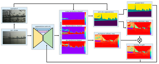
Figure 1.
The diagram of the proposed method.
In order to employ our USV in a complex dynamic environment for various tasks, the perception system is designed to satisfy the following requirements.
- (1)
- Accurate and robust scene perception with each input new image;
- (2)
- Adaptive ability during the navigation in the dynamic environment;
- (3)
- Image is the only input.
A segmentation network model is created for the USV visual perception. The network is initialized with small, manually labeled data. To improve the network prediction accuracy, the CRF algorithm is introduced as a post-process. To further refine the network output, a superpixel map is generated from the original image based on the texture and color similarity. Two criteria are designed to evaluate the prediction confidence of each pixel. The refined network output is regarded as the pseudo label. In order to improve the USV adaptive capacity, a self-training method is proposed to train the network based on the pseudo label and the corresponding weight map.
3.1. Online Deep Learning Segmentation Network
(1) Segmentation network
We draw inspiration from the U-net architecture [31], which is applied for biomedical image segmentation. We design an end-to-end encoder–decoder network for the water image segmentation. Multiple feature maps in different layers are fully utilized, which improves network performance. The encoder layers are based on the VGG [37] network. The VGG architecture consists of several convolutional layers and fully connected layers. The fully connected layers are removed and the convolutional layers are reserved as the feature extraction. The convolutional layers are divided into five stages. The feature maps in the five stages are downsampled to feed into the next stage by pooling operations. The VGG model that is trained with a large amount of data is set as the encoder model, assuming that these convolutional layers have a good ability to extract the features of the input image. The last layer of each stage is regarded as the feature maps and up-sample to feed into the corresponding decoder network. Three other convolutional layers are added after the encoder layers for the pixels classification.
(2) Segmentation pre-train
Before the navigation, we expect that the intelligent USV can recognize the different sceneries based on the texture information. The traditional methods extract a set of features identified by a domain expert according to each application. Then a classifier, such as support vector machine (SVM), is used to predict each region of the input image. Due to the complex variability of the texture, it is hard to design an effective method to extract a valid feature from the complex various texture in the dynamic scene. The traditional methods have limited performance in our application. Moreover, these designed features focus on the local region information and neglect the global structure information of the image.
These problems can be solved effectively by the deep convolutional neural network-based algorithms. The convolutional layers can effectively and automatically learn both the low-level and high-level features. Domain expertise is no longer needed for the hardcore feature extraction. Through experiment analysis, we found that the neural networks learn not only the local feature but also the global semantic relationship between different regions, which increases the robustness of the engaged algorithm.
We use the basic segmentation network to realize the feature extraction and region prediction in this work. As a widespread technique for the network initialization, the basic VGG network that is trained on the ImageNet dataset is set as the encoder network of our architecture. In this step, the network needs further training before it has the ability to segment images.
Before the USV is employed in a new scene that has different color and texture from the historical application scene, several representative scene images are manually labeled into three categories, water, land and sky. Then, we train the network to learn a generic notion of how to learn the features of each category and recognize each region of the images. Stochastic gradient descent (SGD) is used to optimize the network with momentum 0.9 for 50,000 iterations. The dataset is randomly augmented by mirroring and zooming to improve the robustness of the feature extraction. After offline training, the network can roughly segment the input image base on the learned feature.
(3) Segmentation result refinement
CRF is an effective way to refine the multi-class object segmentation by considering the relationship with adjacent pixels [38]. Motivated by the work with a method that combined CNN and CRF [39], the outputs of the segmentation network are improved by the CRF post-process. Let be the random variable of pixel , which represents the label and can take any value from a pre-defined set of labels . Let X be the vector formed by the random variables , where N is the number of pixels in the image. Let be input image data. The optimization of the CRF model is defined by the energy function:
The formula consists of two parts, the unary potentials and the pairwise potentials . measure the inverse likelihood of the pixel taking the label without considering the smoothness and the consistency of the label assignments, which are obtained from the segmentation network output. measure the cost of assigning labels , to pixels ; simultaneously, which encourages assigning similar labels to adjacent pixels with similar properties. It is defined:
where and is the pixel position. represents the compatibility of the labels assigned to variables and , where if and 1 otherwise.
The first term depends on the neighboring information of the pixel positions and the pixel value similarity. The second term only considers the pixel positions. The optimization process is to get the minimum energy E(x) value, which can refine the local segmentation.
3.2. Superpixel-Level Pseudo Label Generation
After the segmentation network prediction and the CRF refinement, the image is assigned with a class label at the pixel level. A large number of experiment results indicated that pixels with great prediction uncertainty or error prediction mainly locate near the edge of different regions, as is shown in Figure 2. The second column in Figure 2 shows the three category prediction channels. Three prediction values in each pixel are processed by the argmax function to obtain each category prediction probability. Then, the three category prediction values are sorted to get three new prediction channels, shown in the third column. The result in the bottom of the third column illustrates that the prediction has a high probability for the corresponding category except for the pixels near the boundary. The prediction results of the three classes are similar near the boundary, which indicates that the network cannot distinguish the category of these pixels. In order to show the significant degree of different category prediction results, we subtract the largest predicted value from the second-largest value to obtain the prediction contrast map, shown in the fourth column.

Figure 2.
Analysis of prediction results in different regions.
In order to solve the uncertain problem of the local region and boundary prediction, our attempt is to improve the result by applying the superpixel based method. We proposed to cluster pixels with similar characteristics into superpixels. It is assumed that the pixels in the superpixels should be labeled as the same class. In our work, we improve the pseudo label at the superpixel level before the next segmentation training. A graph-based segmentation technique [40] is used to obtain the superpixels in this paper. At the beginning of the graph-based segmentation approach, each pixel is set as a separate region for the initialization. Then, small regions are merged into a large region recursively until certain criteria is met.
The superpixels are expressed as . Then we calculate the pixel number of water, land and sky in each region. For the a superpixel , the category number statistical result is expressed as . , and are the pixel number of water, land and sky respectively in . The class with the largest number of pixels in the region is regarded as the region category:
where is the largest number in . is a function, which is used to find the label corresponding to the largest number in superpixel . is set as the label of .
3.3. Degree of Confidence Evaluation
As the segmentation network is trained automatically without an external guide, we wish to remove the influence of the pixels with error labels and train the network with the pixels with the right label as much as possible. Therefore, two criteria are designed to evaluate the confidence degree of each pixel for the pseudo label. To improve the robustness of the online self-training process, the segmentation network is trained according to these criteria.
(1) Prediction consistency in a region
Ideally, the water, land and sky region have discriminable color and texture features. Most of the pixels in a superpixel should be label as the same class. Regions near the inconspicuous edge would have pixels with various labels. These regions have a great probability of error label. Thus, we use the pixel prediction consistency to judge the prediction confidence in a superpixel. The measurement in a superpixel is expressed as follows.
The prediction consistency measurement stands for the proportion of certain category pixels with the largest number in a region.
(2) Prediction saliency of three categories
As the USV is navigation in the dynamic unknown environment, the trained segmentation network may fail in the new environment. In this new environment, some pixels would have similar prediction probabilities in each category, which makes it hard to measure the category of these pixels. A good prediction is that a specific category prediction probability is near 1 and the other two category prediction probability is near 0. Then, we design an evaluation method to measure the confidence of each pixel prediction. The measurement is defined as:
where represent the reliability of th pixel prediction, is the largest value in the three class prediction channel and is the second-largest value.
The greater the difference between the largest prediction value and the second-largest prediction value, the more convincing the prediction is. For example, if a pixel is predicted as the water, like , the largest prediction value is 1 and the second largest prediction value is 0. Then, according to the formula, the reliability of the prediction is 1, which means the pixel is absolutely the water. To the contrary, if the prediction of a pixel is , the largest prediction value and the second-largest prediction value are the same, which means it is hard to distinguish the category of the pixel. The reliability of the prediction is 0, which means the prediction is incredible. Then, we calculate the mean prediction confidence of a superpixel as:
3.4. Online Training Segmentation Network
During the navigation of the USV, pseudo labels are fed into the network training for self-training. The loss function for the training is defined as:
where is the pseudo label and is the corresponding prediction of the network.
Considering the uncertainty of the pseudo label, pixels with high confidence have large weights to train the network, which is to avoid network degradation during the training. The training weight map is calculated according to the prediction consistency measurement and the prediction saliency measurement .
To remove the influence of the pixel with low confidence, the weight map is processed by an activation function. The activation function is defined as:
.
The loss function is modified as:
The advantage of this loss function is that it puts more weight on pixels with greater label confidence and less weight on those unreliable pixels, hence reduces the degradation of the network caused by the bad training samples.
4. Experimental Results
A set of experiments have been conducted to verify the performance of the proposed method. The experiment data mainly come from the video captured by our USV navigating in East Lake located in Wuhan, China. Our experimental USV and the navigation environment are shown in Figure 3. To further evaluate the adaptive transferability of the proposed method to various new environments, video data captured over the Yangtze River and sea are used in the experiment.
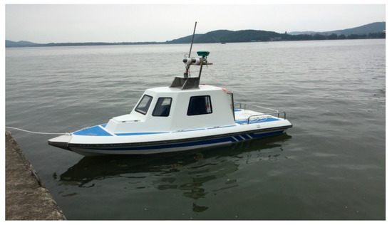
Figure 3.
Our team’s experimental unmanned surface vehicle (USV) at East Lake.
4.1. Evaluation of Online Learning
In order to clearly show the improvement of the network prediction during the process of the pseudo label generating, the segmentation network is pre-trained with bad training data that is added with some stochastic noise. Each region in the label mask is processed by the morphological operations of dilation or erosion randomly. The edge error between each class region is a common problem in the image labeling process. By the artificial expansion of the edge error, it is for the clear demonstration of the region edge refinement in the pseudo generating. Random dot and line noise are also added to demonstrate the local refinement in the pseudo generating. As shown in Figure 4, the first row is the original image; the second row is the correct label; and the last row is the labels mixed with manually added noise.

Figure 4.
Training data with random noise.
The segmentation network is trained with the noise data. Then the trained segmentation network is applied to predict the image of the East Lake. The prediction is refined by the pseudo label generation process. As is shown in Figure 5, the first row is the original image. The second row is the segmentation prediction by the trained segmentation network. The third row is the pseudo label generation result. The experiment shows that our designed post-processing can effectively correct the local error prediction.
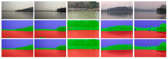
Figure 5.
Refinement of the network prediction.
The metric method of Intersection over Union (IoU) is employed to better understand the quantitative performance of the proposed method. The IoU metric is essentially a method to quantify the percent overlap between the target mask and our prediction output. Namely, the metric measures the number of pixels common between the target and prediction masks divided by the total number of pixels present across both masks. In segmentation tasks, the IoU is preferred over accuracy as it is not as affected by the class imbalance that is inherent in foreground and background segmentation tasks. The IoU is calculated as follows:
where is the ground truth segmentation and is the segmentation prediction. is the successful prediction number when the ground truth is positive. and are the failure prediction number when the ground truths are negative and positive respectively.
Figure 6 shows the IoU result of each class. In this experiment, a short video is labeled as the ground truth. The basic segmentation network trained with noise data is used to predict each image in the video. The lines of water1, land1 and sky1 in the figure are the basic network IoU results of water, land and sky region respectively in the time sequence. Then, the basic segmentation is regarded as the initial network of the online learning network. The network is trained automatically and images are predicted at the same time. The line of water2, land2 and sky2 in the figure is the online learning network IoU result of water, land and sky region respectively. By comparing the online training model with the basic segmentation model, the performance of our proposed network is gradually improved after the self-training. As the water region and the sky region take up a large part of the image, some local failure predictions in these regions play a small role in the water and sky class final IoU result. On the other hand, the land region accounts for a small part in the image and the local failure predictions have a significant influence on the land IoU result. By calculating the mean percentage of the three class quantity in the whole video, we found that the water region accounts for 40.23%, the land region accounts for 16.87% and the sky region accounts for 42.90% of the images. During the navigation of the USV, we pay more attention to the obstacle detection and avoid the obstacle in the local path planning. Therefore, the improvement of the land region prediction plays an important role in the USV environment perception. After continuous online learning, our proposed method could significantly improve land prediction accuracy.

Figure 6.
Performance evaluation of each online learning step.
4.2. Performance in Different Scenes
In this section, five groups of different experiments with different conditions were conducted to verify the feasibility of the proposed algorithm in various complex environments. The experimental conditions are selected according to the distance from the shore. As shown in Figure 7, each row is an image sequence in a specific condition and each image is combined with the original image and segmentation result. The offshore distance from the first row to the fifth row is from far to near.

Figure 7.
Experiment in different conditions.
In the first row, the image sequence was captured when the USV is far away from the land. There is no reflection of the trees, mountains and buildings on the water surface. Besides, because the USV was far away from the land, the scene on the land is very small in the image. In the second and third rows, the image sequences were captured when the USV was closer to the bank than the first row. With the land region increasing, the reflection on the water surface is more obvious. As the influence of the reflection, the boundary between the water area and the land is not obvious in some local regions, shown in the third row. In the fourth and fifth rows, the image sequences were captured near the bank. As the bank is so close to the water area, these images are full of reflection. The trees on the land projects on the water surface and the colors of the water area are the same as that of the trees because of the illumination, which makes it difficult to distinguish the water region from the land region for the traditional method.
These experiments show that the proposed method exhibits excellent performance in different conditions. To further evaluate the proposed method quantitatively, the five videos are manually labeled as the ground truth. The mean IoU of each class is shown in Table 1.

Table 1.
Intersection over Union (IoU) results in each video.
4.3. Trained Model Transfer to a New Environment
The demand for USV continues to increase recently. The USV has to be adaptive to different tasks in various environments. It is inefficient to train a specific model for each task. We expect that the trained model can be adaptive to a new environment, which reduces a lot of work for manual data labeling. In order to verify that the proposed method could be adaptive to new tasks, videos captured at the Yangtze River and sea by the video camera and mobile phone camera are used in the experiment based on the initial model trained by the images data captured in East Lake. The experiment result is shown in Figure 8.

Figure 8.
Model transferred to a new environment.
The images in the first three rows were captured at the Yangtze River in different scenarios. The scene of the first row is at the dock. The background features buildings in the second row and the Yangtze River Bridge in the third row. The images in the last three rows were captured at sea. The images in the fourth row were captured in the evening. The images in the fifth row were captured near the island. The images in the last row were captured far away from the coast, in which the land is small in the images.
We can see from the experiments that the performance of the network is continuously improved during the online self-training. When the USV is driving into a new environment, although the network shows poor performance at the beginning, it constantly corrects the error prediction for a period of self-learning and is finally well adapted to the new environment. Table 2 shows the IoU result of each video after online learning. These experiments prove that the proposed method has a good transferability to different new environments. With this ability, our USV can be deployed to many new tasks without further training. Large work is no longer needed to label new data before each new task. Furthermore, the right predictions that are close to manual labeling can be selected as the ground truth data to increase the ground truth database.
Table 2.
Performance in new environments.
4.4. Comparison to the State-Of-The-Art Methods
This section presents comparative evaluation results of the proposed algorithm and other state-of-the-art methods (SegNet [41], ENet [42], ICNet [43], ContextNet [44], DeepLab-V2 [39] and PSPNet [45]). The compared models and the proposed model are trained with the dataset captured in the East Lake. In order to measure the self-learning ability of the models, we choose a set of data to train these models. In this experiment, only fifteen images are chosen for training. For the test experiment, we divide the database into three categories, namely, East Lake dataset, Yangtze River dataset and the sea dataset. The East Lake dataset is used to validate the self-improvement during the online learning of the proposed method. The Yangtze River dataset and the sea dataset is used to show model transferability in a different environment. Then, each class IoU is calculated to test these models.
Table 3 shows the comparative results of different methods. Our proposed method outperforms the other approaches in all the datasets. The performances of some reference models heavily depend on the training data set. They have a good prediction only in the condition that they have learned from large training data. When the models are used in the new environment, they have poor performance as the texture and illumination are different from the training dataset. As shown in Table 3, these models have a relatively good performance at the Yangtze River, because the texture at the Yangtze River is similar to the texture at the East Lake. On the contrary, they have poor performance at sea, because the texture at sea has a large difference from that at the East Lake. While our model has the ability to train itself, its performance is limited in the beginning. Only after a few steps of self-training, our model can be stably adaptive to the new environment.
Table 3.
Comparative experimental results.
5. Conclusions
In this paper, an adaptive semantic segmentation is proposed for the visual perception of the USV autonomous navigation. The segmentation algorithm is based on the encoder–decoder convolutional neural network. CRF as a post-process is added after the network to improve the network prediction accuracy. In order to avoid the dependence on a large amount of manually labeled data for the network performance, an online self-training method is put forward. The network is pre-trained with a small labeled data and gradually improved by the self-training. A superpixel based refinement algorithm is used to generate the pseudo label for self-training. Two uncertainty evaluation criteria that measure the confidence of each pixel prediction are designed to guide the network training by removing the influence of the pixels with error labels and rewarding the training with the right label. A set of experiments were conducted to test the proposed method in the river, lake and sea. These experiments indicate that the proposed method can get rid of the dependence on a large number of training data for high performance. Like other network models, our approach has limited performance after training with small training data. It can be gradually improved after a few steps of self-training. These experiments also show that the proposed method has an excellent adaptivity to a new environment, very attractive for the applications in many different environments.
Author Contributions
Conceptualization, W.Z., C.X. (Changshi Xiao) and Q.L.; methodology, Y.W. and C.Z.; software, S.X.; validation, X.Z. and C.X. (Changshi Xiao); formal analysis, C.X. (Changshi Xiao) and Q.L.; investigation, Y.W. and H.Y.; writing—original draft preparation, X.Z. and C.X. (Cheng Xie); writing—review and editing, S.X. and C.X. (Cheng Xie). All authors have read and agreed to the published version of the manuscript.
Funding
This work is supported by the National Science Foundation of China (NSFC) through Grant No. 51679180, Wuhan University of Technology Independent Innovation Research Foundation of China through Grant No. 2018III059GX, Hubei Provincial Natural Science Foundation of China through Grant No. 2016CFB362, and Double First-rate Project of WUT. Q. Li acknowledges the support of Virginia Microelectronics Consortium (VMEC) Chair professor grant.
Conflicts of Interest
The authors declare no conflict of interest.
References
- Kristan, M.; Kenk, V.S.; Kovačič, S.; Perš, J. Fast image-based obstacle detection from unmanned surface vehicles. IEEE Trans. Cybern. 2015, 46, 641–654. [Google Scholar] [CrossRef]
- Stateczny, A.; Kazimierski, W.; Burdziakowski, P.; Motyl, W.; Wisniewska, M. Shore Construction Detection by Automotive Radar for the Needs of Autonomous Surface Vehicle Navigation. ISPRS Int. J. Geo-Inf. 2019, 8, 80. [Google Scholar] [CrossRef]
- Stateczny, A.; Kazimierski, W.; Gronska-Sledz, D.; Motyl, W. The Empirical Application of Automotive 3D Radar Sensor for Target Detection for an Autonomous Surface Vehicle’s Navigation. Remote Sens. 2019, 11, 1156. [Google Scholar] [CrossRef]
- Praczyk, T. A quick algorithm for horizon line detection in marine images. J. Mar. Sci. Technol. 2018, 23, 164–177. [Google Scholar] [CrossRef]
- Ji, Z.; Su, Y.; Wang, J.; Hua, R. Robust sea-sky-line detection based on horizontal projection and hough transformation. In Proceedings of the 2009 2nd International Congress on Image and Signal Processing, Tianjin, China, 17–19 October 2009; pp. 1–4. [Google Scholar]
- Gershikov, E.; Baskin, C. Efficient Horizon Line Detection Using an Energy Function. In Proceedings of the International Conference on Research in Adaptive and Convergent Systems, Krakow Poland, 20–23 September 2017; pp. 110–115. [Google Scholar]
- Zhan, W.; Xiao, C.; Wen, Y.; Zhou, C.; Yuan, H.; Xiu, S.; Zhang, Y.; Zou, X.; Liu, X.; Li, Q. Autonomous Visual Perception for Unmanned Surface Vehicle Navigation in an Unknown Environment. Sensors 2019, 19, 2216. [Google Scholar] [CrossRef] [PubMed]
- Cai, C.T.; Weng, X.Y.; Zhu, Q.D. Sea-skyline-based image stabilization of a buoy-mounted catadioptric omnidirectional vision system. EURASIP J. Image Video Process. 2018, 2018, 1. [Google Scholar] [CrossRef]
- Gershikov, E.; Libe, T.; Kosolapov, S. Horizon line detection in marine images: Which method to choose? Int. J. Adv. Intell. Syst. 2013, 6, 79–88. [Google Scholar]
- Praczyk, T. Artificial neural networks application in maritime, coastal, spare positioning system. Theor. Appl. Inform. 2006, 18, 1175–1189. [Google Scholar]
- Praczyk, T. Neural anti-collision system for Autonomous Surface Vehicle. Neurocomputing 2015, 149, 559–572. [Google Scholar] [CrossRef]
- Ji, Z.; Yu, X.; Pang, Y. Zero-Shot Learning with Deep Canonical Correlation Analysis. In Proceedings of the CCF Chinese Conference on Computer Vision, Tianjin, China, 11–14 October 2017; pp. 209–219. [Google Scholar]
- Ji, Z.; Xiong, K.; Pang, Y.; Li, X. Video summarization with attention-based encoder-decoder networks. IEEE Trans. Circuits Syst. Video Technol. 2019. [Google Scholar] [CrossRef]
- Zhan, W.; Xiao, C.; Yuan, H.; Wen, Y. Effective waterline detection for unmanned surface vehicles in inland water. In Proceedings of the 2017 Seventh International Conference on Image Processing Theory, Tools and Applications (IPTA), Montreal, QC, Canada, 28 November–1 December 2017; pp. 1–6. [Google Scholar]
- Gershikov, E. Is color important for horizon line detection? In Proceedings of the 2014 International Conference on Advanced Technologies for Communications (ATC 2014), Hanoi, Vietnam, 15–17 October 2014; pp. 262–267. [Google Scholar]
- Yongshou, D.; Bowen, L.; Ligang, L.; Jiucai, J.; Weifeng, S.; Feng, S. Sea-sky-line detection based on local Otsu segmentation and Hough transform. Opto-Electron. Eng. 2018, 45, 180039. [Google Scholar]
- Jiang, C.; Jiang, H.; Zhang, C.; Wang, J. A new method of sea-sky-line detection. In Proceedings of the 2010 Third International Symposium on Intelligent Information Technology and Security Informatics, Jinggangshan, China, 2–4 April 2010; pp. 740–743. [Google Scholar]
- Lu, J.-W.; Dong, Y.-Z.; Yuan, X.-H.; Lu, F.-L. An algorithm for locating sky-sea line. In Proceedings of the 2006 IEEE International Conference on Automation Science and Engineering, Shanghai, China, 8–10 October 2006; pp. 615–619. [Google Scholar]
- Liang, D.; Zhang, W.; Huang, Q.; Yang, F. Robust sea-sky-line detection for complex sea background. In Proceedings of the 2015 IEEE International Conference on Progress in Informatics and Computing (PIC), Nanjing, China, 18–20 December 2015; pp. 317–321. [Google Scholar]
- Zafarifar, B.; Weda, H. Horizon detection based on sky-color and edge features. In Proceedings of the Visual Communications and Image Processing 2008, San Jose, CA, USA, 27–31 January 2008; p. 682220. [Google Scholar]
- Shen, Y.-F.; Krusienski, D.; Li, J.; Rahman, Z.-U. A hierarchical horizon detection algorithm. IEEE Geosci. Remote Sens. Lett. 2012, 10, 111–114. [Google Scholar] [CrossRef]
- Wang, H.; Wei, Z.; Wang, S.; Ow, C.S.; Ho, K.T.; Feng, B. A vision-based obstacle detection system for unmanned surface vehicle. In Proceedings of the 2011 IEEE 5th International Conference on Robotics, Automation and Mechatronics (RAM), Qingdao, China, 17–19 September 2011; pp. 364–369. [Google Scholar]
- Yan, Y.; Shin, B.; Mou, X.; Mou, W.; Wang, H. Efficient horizon detection on complex sea for sea surveillance. Int. J. Electr. Electron. Data Commun. 2015, 3, 49–52. [Google Scholar]
- Sun, Y.; Fu, L. Coarse-Fine-Stitched: A Robust Maritime Horizon Line Detection Method for Unmanned Surface Vehicle Applications. Sensors 2018, 18, 2825. [Google Scholar] [CrossRef]
- Yuan, H.; Xiao, C.; Xiu, S.; Zhan, W.; Ye, Z.; Zhang, F.; Zhou, C.; Wen, Y.; Li, Q. A Hierarchical Vision-Based UAV Localization for an Open Landing. Electronics 2018, 7, 68. [Google Scholar] [CrossRef]
- Yuan, H.; Xiao, C.; Xiu, S.; Zhan, W.; Ye, Z.; Zhang, F.; Zhou, C.; Wen, Y.; Li, Q. A hierarchical vision-based localization of rotor unmanned aerial vehicles for autonomous landing. Int. J. Distrib. Sens. Netw. 2018, 14, 1550147718800655. [Google Scholar] [CrossRef]
- Jeong, C.; Yang, H.S.; Moon, K. A novel approach for detecting the horizon using a convolutional neural network and multi-scale edge detection. Multidimens. Syst. Signal Process. 2019, 30, 1187–1204. [Google Scholar] [CrossRef]
- Jeong, C.Y.; Yang, H.S.; Moon, K.D. Horizon detection in maritime images using scene parsing network. Electron. Lett. 2018, 54, 760–761. [Google Scholar] [CrossRef]
- Steccanella, L.; Bloisi, D.; Blum, J.; Farinelli, A. Deep Learning Waterline Detection for Low-Cost Autonomous Boats. In Proceedings of the International Conference on Intelligent Autonomous Systems, Baden-Baden, Germany, 11–15 June 2018; pp. 613–625. [Google Scholar]
- Long, J.; Shelhamer, E.; Darrell, T. Fully convolutional networks for semantic segmentation. In Proceedings of the IEEE Conference on Computer Vision and Pattern Recognition, Boston, MA, USA, 7–12 June 2015; pp. 3431–3440. [Google Scholar]
- Ronneberger, O.; Fischer, P.; Brox, T. U-net: Convolutional networks for biomedical image segmentation. In Proceedings of the International Conference on Medical Image Computing and Computer-Assisted Intervention, Munich, Germany, 5–9 October 2015; pp. 234–241. [Google Scholar]
- Lucchi, A.; Li, Y.; Boix, X.; Smith, K.; Fua, P. Are spatial and global constraints really necessary for segmentation? In Proceedings of the 2011 International Conference on Computer Vision, Barcelona, Spain, 6–13 November 2011; pp. 9–16. [Google Scholar]
- He, K.; Zhang, X.; Ren, S.; Sun, J. Delving deep into rectifiers: Surpassing human-level performance on imagenet classification. In Proceedings of the IEEE International Conference on Computer Vision, Santiago, Chile, 7–13 December 2015; pp. 1026–1034. [Google Scholar]
- Chen, L.-C.; Papandreou, G.; Kokkinos, I.; Murphy, K.; Yuille, A.L. Semantic image segmentation with deep convolutional nets and fully connected crfs. In Proceedings of the 2015 IEEE International Conference on Computer Vision (ICCV 2015), Santiago, Chile, 7–13 December 2015. [Google Scholar]
- Zheng, S.; Jayasumana, S.; Romera-Paredes, B.; Vineet, V.; Su, Z.; Du, D.; Huang, C.; Torr, P.H. Conditional random fields as recurrent neural networks. In Proceedings of the IEEE International Conference on Computer Vision, Santiago, Chile, 7–13 December 2015; pp. 1529–1537. [Google Scholar]
- Visin, F.; Ciccone, M.; Romero, A.; Kastner, K.; Cho, K.; Bengio, Y.; Matteucci, M.; Courville, A. Reseg: A recurrent neural network-based model for semantic segmentation. In Proceedings of the IEEE Conference on Computer Vision and Pattern Recognition Workshops, Las Vegas, NV, USA, 27–30 June 2016; pp. 41–48. [Google Scholar]
- Simonyan, K.; Zisserman, A. Very deep convolutional networks for large-scale image recognition. arXiv 2014, arXiv:1409.1556. [Google Scholar]
- Krähenbühl, P.; Koltun, V. Efficient inference in fully connected crfs with gaussian edge potentials. Adv. Neural Inf. Process. Syst. 2011, 24, 109–117. [Google Scholar]
- Chen, L.-C.; Papandreou, G.; Kokkinos, I.; Murphy, K.; Yuille, A.L. Deeplab: Semantic image segmentation with deep convolutional nets, atrous convolution, and fully connected crfs. IEEE Trans. Pattern Anal. Mach. Intell. 2018, 40, 834–848. [Google Scholar] [CrossRef] [PubMed]
- Felzenszwalb, P.F.; Huttenlocher, D.P. Efficient graph-based image segmentation. Int. J. Comput. Vis. 2004, 59, 167–181. [Google Scholar] [CrossRef]
- Badrinarayanan, V.; Kendall, A.; Cipolla, R. Segnet: A deep convolutional encoder-decoder architecture for image segmentation. IEEE Trans. Pattern Anal. Mach. Intell. 2017, 39, 2481–2495. [Google Scholar] [CrossRef] [PubMed]
- Paszke, A.; Chaurasia, A.; Kim, S.; Culurciello, E. Enet: A deep neural network architecture for real-time semantic segmentation. arXiv 2016, arXiv:1606.02147. [Google Scholar]
- Zhao, H.; Qi, X.; Shen, X.; Shi, J.; Jia, J. Icnet for real-time semantic segmentation on high-resolution images. In Proceedings of the European Conference on Computer Vision (ECCV), Munich, Germany, 8–14 September 2018; pp. 405–420. [Google Scholar]
- Poudel, R.P.; Bonde, U.; Liwicki, S.; Zach, C. Contextnet: Exploring context and detail for semantic segmentation in real-time. arXiv 2018, arXiv:1805.04554. [Google Scholar]
- Zhao, H.; Shi, J.; Qi, X.; Wang, X.; Jia, J. Pyramid scene parsing network. In Proceedings of the IEEE Conference on Computer Vision and Pattern Recognition, Honolulu, HI, USA, 21–26 July 2017; pp. 2881–2890. [Google Scholar]
© 2020 by the authors. Licensee MDPI, Basel, Switzerland. This article is an open access article distributed under the terms and conditions of the Creative Commons Attribution (CC BY) license (http://creativecommons.org/licenses/by/4.0/).