Development of a Portable Multi-Sensor Urine Test and Data Collection Platform for Risk Assessment of Kidney Stone Formation

Abstract

In this paper, we present an Internet of things (IoT)-based data collection system for the risk assessment of urinary stone formation, or urolithiasis, by the measurement and storage of four parameters in urine: pH, concentrations of ionized calcium (Ca²⁺), uric acid and total dissolved solids. The measurements collected by the system from patients and healthy individuals grouped by age and gender will be stored in a cloud database. These will be used in the training phase of an artificial intelligence (AI) machine learning process utilizing the logistics regression model. The trained model provides a binary risk assessment, indicating if the end user is either a stone-former or not. For system validation, standard chemical solutions were used. Preliminary results indicated a sufficient measurement range, falling within the physiological range, and resolution for pH (2.0–10.0, +/−0.1), Ca²⁺(0.1–3.0 mmol/l, +/−0.05), uric acid (20–500 ppm, +/−1) and conductivity (1.0–40.0 mS/cm, +/−0.1), exhibiting high correlation with standard instruments. We intend to deploy this system in few hospitals in Taiwan to collect the data of patients’ urine, with analysis aided by urologist assessments for the risk of urolithiasis. The modularized design allows future modification and expansion to accommodate other sensing analytes.

1. Introduction

In recent decades, the occurrence rate of urolithiasis (i.e., the formation of urinary stones) is increasing in most countries worldwide [1]. Research in the United States shows a 1.9 time increase in the rate of urolithiasis, according to emergency department visits between 1992 and 2009 [2]. The expenses associated with stone diseases include public health and an economic burden exceeding $10 billion in the United States [3]. Another study in Iceland for a duration of 24 years reported a significant increase in the incidence of kidney stone diseases [4]. In the 2019 report of annual medical expenses from Taiwan National Health Insurance, chronic kidney disease stayed on top of the list, accounting for more than USD 1.7 billion [5].

Kidney stone formation remains asymptomatic until the final stages, when there is the presence of blood in the urine, painful urination or pain in the back or lower abdomen [6]. In this stage, medical imaging such as the conventional X-ray, computed tomography (CT) or multi-detector CT is used for detecting the size and location of the stone. In addition to size and location, the composition of the stone, its fragility and patient symptoms influence the urologist’s decision for treatment. The treatment could be urologic intervention or medical therapy [7].

Details of the prognosis and factors for urolithiasis progression, as well as comparisons between different methods of stone formation risk assessment based on urine composition, are presented in [1]. Although stone removal solves the patient’s immediate problem, it is not a cure for the abnormality that caused the formation of the stone [1]. In many cases, patients often experience the recurrence of urinary stones. Several methods for assessing the risk factor of stone formation based on urine composition are presented in [1]. These include the BONN Risk Index, which requires only two measurements, Tiselius indices and Robertson Risk Factor Algorithms (RRFA) methods, which rely on seven measurements, and some other methods requiring 12–14 measurements. The comparison between different methods in [1] evaluated the trade-off between the number of measurements and the detection of stones. Monitoring the urine composition allows for correcting the abnormality using classic methods such as metabolic screening, appropriate diet or medical management. Furthermore, urine composition could be used for determining the formation of stones [1].

The recent advances in Internet of things (IoT) devices for the healthcare sector [8] allowed the development of systems with extended abilities for the monitoring, storage and analysis of large amounts of data in a short period of time. The presented system in this paper provides three essential roles—data collection, data storage, and binary risk assessment—organized in a centralized database and performed in the cloud. Such data will be used in a machine learning training process to create the model for assessing urinary stone formation risk. After the training phase and model development, the system will be utilized as a point-of-care device for the risk assessment of urinary stone formation in the early stages.

Although urinary stones are found in a variety of compositions, studies reported in [9,10] on stone compositions showed that more than 70% of stones are made from calcium oxalate (CaOx) or combinations of CaOx with other minerals containing calcium ions. There is potential in predicting urinary stone formation by measuring only the conductivity and using this prediction technique at home [11]. Our system, meanwhile, incorporated four measurands, namely pH, ionized calcium (Ca²⁺), uric acid concentration and conductivity, with the corresponding readout circuits adopted from the on-chip multi-sensor interface from [6]. In addition to the sensor readout circuits, we included on-board computing and wireless connectivity, thereby forming a complete solution for point-of-care applications. In this paper, a system based on flexible modular design is selected to address the data collection challenges by adding internet connectivity while enhancing the circuit design presented in [6]. These measurands have, in part or collectively, been used for the metabolic screening of urine [1]. A multi-analyte approach can cater to more predictive ability that is vital for detecting the onset of stone progression. The noninvasive nature of urine sample analysis, combined with IoT capability, results in an information-rich database containing several patients’ data with cloud-based computing for primordial risk assessment.

The system is designed to have the flexibility of connecting to different types of sensor configurations. The potentiometric readout circuit utilizes field effect transistor (FET)-based sensors in the form of ion-sensitive field effect transistor (ISFETs) and enzyme-extended gate FETs (EEGFETs) for the measurement of pH and ionized calcium (Ca²⁺), respectively. The detailed specification of an ISFET pH sensor and the corresponding potentiometric readout circuit are presented in [12]. The readout circuit is based on a floating bridge, constant-voltage, constant-current source. The same base design with minor enhancements is used in the system presented in this paper. The amperometric readout circuit, which has the ability to measure uric acid concentration, could be used by a two-electrode or three-electrode electrochemical cell. Two implementations of an amperometric sensor readout circuit are presented in [13]. The readout topology, which uses a P-channel metal-oxide-semiconductor (PMOS) at its input, has a wider range of current sensing, compared with those reported circuits using transimpedance amplifiers [13]. We have derived a simplified version of this readout circuit topology for ease of device integration. The multi-frequency conductivity measurement readout circuit is based on the circuit used in [6] and has the flexibility of measuring the electrical conductivity of a urine sample by a two-electrode or four-electrode conductivity sensor. The measurement of electrical conductivity is used for the detection of the level of total dissolved solids in a urine sample. The relevance between urine sample conductivity and total dissolved solids is shown in [14]. The system also measures the temperature using a semiconductor temperature sensor. The temperature data is used for improving the accuracy of the measurement of other parameters. The digital back end of the system is an ARM^® Cortex-M0+^® microcontroller with an 8-channel 12-bit analog-to-digital converter (ADC) that has a maximum sampling rate of 1 mega sample per second (MSPS). The microcontroller acts as the brain of the system. It controls the whole process by properly providing the required digital and analog signals for each readout circuit. In addition, the output signals from the readout circuits are conditioned prior to connecting to the microcontroller’s embedded ADC. The measured value of the ADC was later calibrated by the pre-stored factors and temporarily saved in the microcontroller’s memory. The single board computer, a Raspberry Pi^® Model 3B, communicates with the microcontroller through the serial port to collect the results and store them in the single board computer’s local database. Furthermore, Internet connectivity, the access point and the local HTML server, which form the graphic user interface (GUI) and data synchronization in the cloud, are parts of the system handled by the single board computer.

The measurement range of each parameter has been selected to cover the physiological range expected form healthy individuals and from those who are suffering from urolithiasis. The study published in [15] reported that patients who formed uric acid stones most commonly had a persistently low urine pH less than 5.5. Hypercalciuria was diagnosed for calcium excretions exceeding 4 mg/kg/24 h [16]. Meanwhile, urinary pH is the main determinant of uric acid crystallization and precipitation and, in fact, the vast majority of uric acid stones are associated with a low urine pH, rather than the excessive urinary concentration of uric acid due to hyperuricosuria and low urine volume. The risk of uric acid crystallization increases proportionally with a progressive fall in urine pH [17]. Based on the reports from [14], the values of electrical conductivity (EC) ranged from 1.1 to 33.9 mS/cm, the mean value being 21.5 mS/cm. The total dissolved solids (TDS) ranged from 3028 ppm to 18,480 ppm, the mean value being 7012 ppm. The TDS levels corresponded with the EC of urine.

The on-board design and the use of off-the-self commercial components and sensors accelerated the implementation of the overall system concept for immediate practical deployment. Attempts to develop the chips required more time and a relatively bigger budget. However, it has the potential for a smaller form factor, low power and a fully integrated system. A first version of our multi-sensor analog front-end chip for interfacing to multiple sensors is presented in [6].

The IoT-enabled design of the system allows for distributing multiple devices to different locations, then collecting measurement results from multiple samples simultaneously and storing them in a central database. This configuration makes the access to a large amount of data in a short period of time possible. In the first phase, the data will be used in an artificial intelligence machine learning training process. Once a urine sample is supplied to the system for the measurement of four parameters, the urologist, physician or medical personnel assesses whether the individual is a stone-former or not. Their assessment is based on background history, symptoms, their expert analysis of the urine sample and other diagnosis tools. A logistics regression model is selected, since it is more suitable for systems that require only a binary output. The output of the model has two states indicating if the person has a high risk of forming kidney stones or a low risk of urinary stone formation. The model’s six inputs are the four measured parameters along with gender and age. Upon validating the trained model, the system will serve as a portable point-of-care device. In this stage, the system will measure the same four parameters from a urine sample and feed them to the trained model, along with the age and gender of the person. The output from the model will indicate if the person is at a high risk of forming kidney stones. Meanwhile, the information in the central database becomes richer, as the data from IoT-enabled point-of-care devices will be saved in database, too. This feature allows for the re-evaluation and improvement of the initial model in the future with a larger data set.

2. Materials and Methods

The system measured four parameters—pH, Ca²⁺, uric acid concentration and conductivity—of the sample from the first void urine in the morning, based on the method performed in [11]. By taking the first void urine in the morning, we could further assess the possibility of stone formation, because such urine has stayed for a relatively longer time in the urinary tract. Moreover, at nighttime, the body is in a relatively dehydrated status.

In the previous approaches of system implementation, the on-board module was designed for single-parameter measurement. Figure 1 shows the on-board implementation from [11], used for the measurement of urine sample conductivity.

The on-board implementation of the potentiometric circuit presented in [18] was used for measuring the pH and Ca²⁺ in urine samples, as shown in Figure 2.

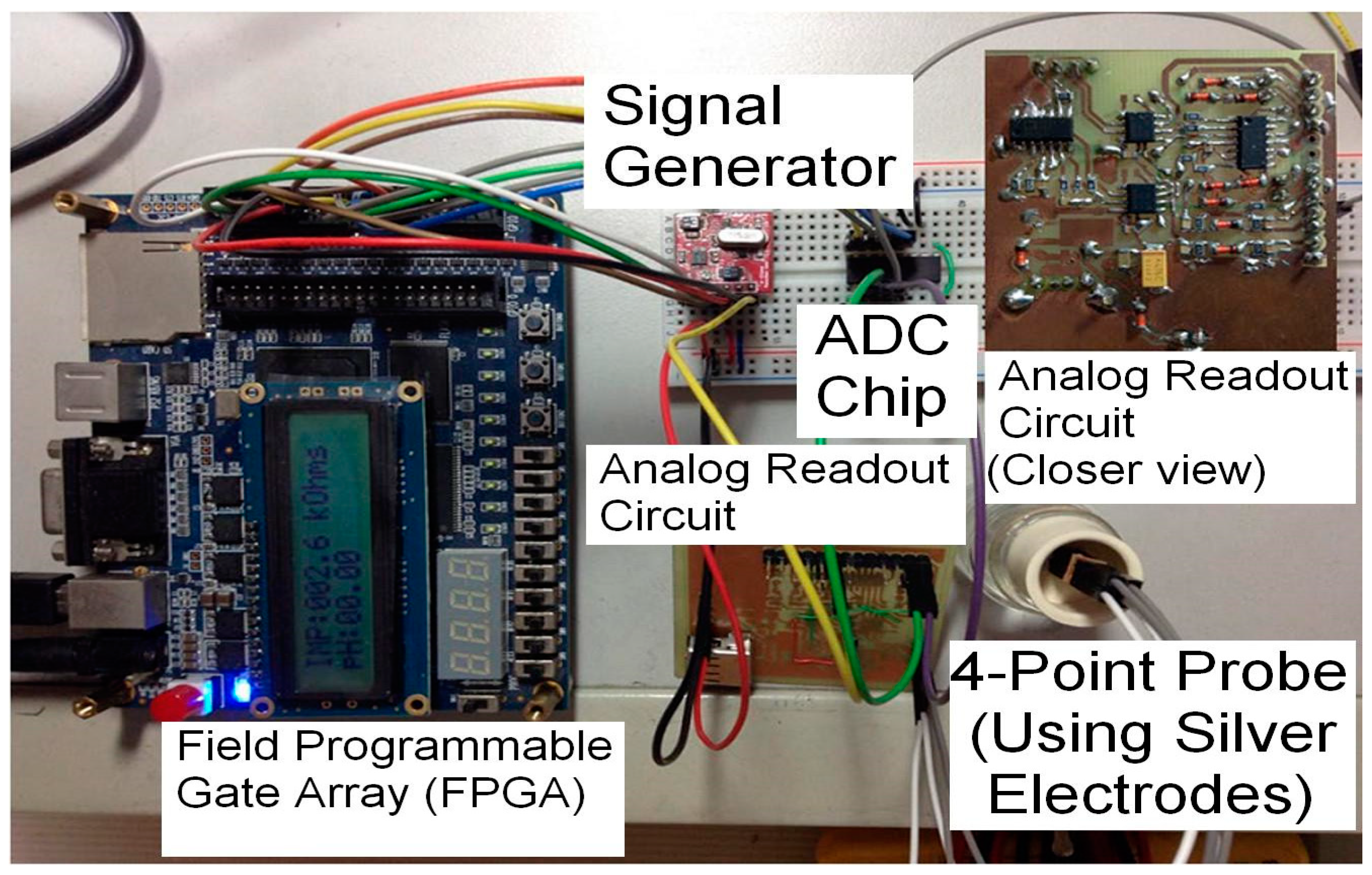
Since in the design of our system flexibility was considered a major feature, modular design was utilized. The sensors were separated and connected to the system using cables. This allowed the electronic circuits to remain inside an enclosure without exposure to the outside environment. Each readout circuit was implemented on an independent printed circuit board (PCB), while the digital controller and single-board computer were independent modules as well. A motherboard with proper sockets and connectors was used for the assembly of the system and connecting different modules to each other, as shown in Figure 3.

The block diagram of the system is shown in Figure 4. There were four layers in the system. The sensor layer included an ISFET sensor for pH measurement, an EEGFET sensor for measuring the Ca²⁺ concentration, an electrochemical cell formed the uric acid level sensor, a gold-coated four-electrode conductivity sensor and a semiconductor temperature sensor. The measurement of the ambient temperature was required for the calibration process, as most of the measuring parameters were temperature-sensitive.

The readout circuits were the next layer of the system. The potentiometric readout circuit was connected to the pH and Ca²⁺ sensors via a selector relay. The uric acid level was measured by an amperometric readout circuit connected to an electrochemical cell. The conductivity sensor was connected to a multi-frequency conductometric readout circuit for the measurement of conductivity.

The digital backend was the next layer of system that controlled the whole system’s operation, as well as digitizing the analog output of the readout circuits. Calibration, including temperature compensation and linearization, was performed digitally in the microcontroller.

The last layer, the single-board computer, communicated with the microcontroller to collect the measured data and send the user commands, as well as configuration and setting parameters. It had the local database for the storage of measured data. Its local HTML server provided a GUI that allowed the user to connect with the system via a smart phone, laptop or computer. It also provided Wi-Fi connectivity as an access point in the absence of an Internet connection. The synchronization of data between the local database and the centralized database in the cloud would be executed whenever an Internet connection was available.

The system was energized by a 5 V rechargeable power bank with multiple USB power connectors. The power bank had enough capacity for operation of the whole system during testing, setting, calibration and data synchronization.

2.1. Redaout Circuits

2.1.1. Potentiometric Readout Circuit

This readout circuit was used for measuring the pH and Ca²⁺ concentrations through the ISFET and EEGFET sensors. Such a sensor has an output related to ion activity once it is biased in the linear region, as the voltage and current should remain constant with a predefined value during the test:

$$I_{DS}={\mu }_n{C}_{ox}\frac{W}{L}\left[\left(V_{GS}-V_{TH(ISFET)}\right)V_{DS}-\frac{1}{2}{V}_{DS}^2\right]$$

(1)

Equation (1) is the conventional model of a MOSFET device in a linear region, where I_DS is the drain–source current, V_GS is the gate–source voltage, V_DS is the drain–source voltage, µ_n is the mobility of electron carriers in the semiconductor layer, W and L are the width and length of the channel, respectively and V_TH is the threshold voltage. While in the regular MOSFET model the threshold voltage is constant, Equation (2) shows that in the ISFET and EEGFET, the threshold voltage consists of two components:

$$V_{TH(ISFET)}=V_{TH(MOSFET)}-V_{CHEMICAL}$$

(2)

where V_TH(ISFET) is overall threshold voltage of the sensor, V_TH(MOSFET) is the inherent MOSFET structure threshold voltage and V_CHEMICAL is the electrochemically induced voltage, and its value depends on ion activity and other chemical properties. By combining Equations (1) and (2) and rearranging them, we have the formula for V_GS, as shown in Equation (3):

$$V_{GS}=\frac{I_{DS}}{{\mu }_n{C}_{ox}\frac{W}{L}{V}_{DS}}+V_{TH(MOSFET)}-V_{CHEMICAL}+\frac{1}{2}{V}_{DS}$$

(3)

In order to keep the operation of the sensor in the linear region, we should have had V_DS < (V_GS − V_TH). Furthermore, V_DS and I_DS should remain constant. Satisfying these conditions allowed for the measurement of ion activities (pH and Ca²⁺ concentration) through the V_GS voltage variation [12].

The circuit in Figure 5 acted as a floating bridge, constant-voltage constant-current source. This configuration allowed for the measurement of each ISFET and EEGFET sensor in the array by simply switching to the drain or source while the reference electrode remained connected to the ground.

In the circuit of Figure 5, V_DS equaled the voltage drop across R₂, and I_DS equaled the current passing through R₃. In order to keep those values constant, a feedback from the output voltage was added to the fixed reference voltage and fed through the V₁ point. This configuration kept the voltage difference between V₁ and V_out constant and equal to V_ref during the measurement.

2.1.2. Amperometric Readout Circuit

The amperometric circuit is shown in Figure 6. In order to measure the uric acid concentration, the uric acid sensor needed to be excited by a predefined oxidation voltage before dropping the urine sample on the strip. V_bias is the voltage applied to the readout circuit for generating the oxidation voltage in the sensor:

$$V_{ox}=V_{DD}-V_{bias}$$

(4)

The relationship between the oxidation voltage V_ox and the bias voltage V_bias is shown in Equation (4). The circuit was a simplified version of the work presented in [13].

Refer to the schematic diagram in Figure 6. The op-amp regulated the M₃ gate voltage in such a way that the voltage in the reference electrode (RE) became equal to V_bias. The oxidation voltage V_ox was applied between the working electrode (WE) and the RE. The presence of a urine sample on sensor strip, combined with the applied oxidation voltage, created the sensor current i_Sensor. The same current passed through the drain–source M₃ and M₁. M₁ and M₂ formed a current mirror. By choosing M₁ and M₂ values identical the output current, i_OUT became equal to i_Sensor:

$$i_{sensor}=\frac{V_{DD}-V_{out}}{R_{out}}$$

(5)

The current passed through R_out and created the output voltage proportional to the sensor current, as shown in Equation (5). The measurement of the current was time-sensitive, as the sensor current increased sharply after dropping of the sample and decayed exponentially. The sharp rise of the current, considered as the reference time and actual current measurement, should be performed after a specific delay. There was a trade-off in selecting the delay; a shorter delay caused measuring during an unstable transient time, while a long delay reduced the accuracy due to the decay of the sensor current.

The sensor current measured after a proper delay was proportional to the uric acid concentration in the sample. The complex process of timing and calibration was performed by a digital microcontroller, while the readout circuit applied the oxidation voltage and converted the sensor current to a measurable voltage for the ADC.

2.1.3. Conductometric Readout Circuit

The conductivity readout circuit consisted of three signal conditioning sections, as shown in Figure 7. The first section converted the received digital pulse width modulation (PWM) signal from the microcontroller to a sinusoidal constant current. The second section received the input signal from the sensor voltage electrodes, and it would be connected to the microcontroller ADC input after amplification and filtering. The third section was similar to the second section, except it received its input signal from a shunt resistor in a series with the sensor current feed circuit. The impedance measurement was performed by dividing the root mean square (RMS) value of the voltage by the current.

The system measured the impedance in several frequencies, and the linear regression line of the impedances in different frequencies was calculated. As shown in Figure 8, the Y-intercept of the linear regression (at zero frequency) was the sample resistance. The conductance was obtained by inversing the resistance, and after multiplying it by the cell constant, the conductivity would be calculated.

2.2. Digital Control

The digital back end of the system was a 32-bit Cortex-M0+ ARM^® microcontroller. It had an 8-channel 12-bit successive approximation register (SAR) ADC with a conversion rate up to 1 MSPS. It controlled the whole process of measurement, calibration and adjustment while performing communication with the local server to record the results in the database. Figure 9 shows the connection between the digital control module and the readout circuits.

2.2.1. Communication

The digital system used American Standard Code for Information Interchange (ASCII) communication with the local server through universal asynchronous receiver-transmitter (UART) ports. It received a few commands as single-character inputs and sent data out through ASCII messages. Figure 10 shows the communication block of the digital system.

2.2.2. Analog-to-Digital Converter (ADC)

Six channels of the ADC were used for measuring different parameters in the system, as shown in Figure 11. Three channels of the ADC were time-insensitive. Measuring the voltage from the temperature sensor and the output of the potentiometric readout circuit for pH and Ca²⁺ concentrations was straight forward. The conductivity readout circuit had two sinusoidal outputs proportional to the voltage and current of the conductivity sensor. These sine waves needed to be sampled every 4 us alternatively. The amperometric readout circuit output voltage and bias voltage feedback were sampled by the ADC every 100 ms. The conductivity and amperometric output signal measurements were time-sensitive, so both the timing and the ADC resolution contributed to the accuracy of the measurement.

2.2.3. Adjustable Bias Voltage Generator

The digital system generated a PWM, signal shown in Figure 12, which was used by the amperometric readout circuit as a bias voltage after passing it through a low-pass filter. This bias voltage determined the oxidation voltage applied to the uric acid biosensor. Therefore, it should be adjustable, and this would be applied by the digital system through adjusting the duty cycle of the PWM signal.

2.2.4. Sine Wave Generator

In the conductivity readout circuit, the sine wave was generated by filtering a quasi-square signal. This signal was made from two PWM signals, shown in Figure 13, provided by the digital system. The signals passed through the level shifter, analog filters and V-to-I circuit and became the sinusoidal current applied to the conductivity sensor.

2.3. Local Server

The local server was a Raspberry Pi^® Model 3B single-board computer. It had a Wi-Fi module that allowed connection to the Internet and served as an access point in the absence of Internet access. Although, in addition to Wi-Fi, the wired Ethernet connection also could be used; however, the Wi-Fi was preferred since it allowed communication while avoiding exposing the internal circuitry to the clinical and hospital environment.

Database

The measurement data and other related information would be stored in a database. Each system kept a copy of database in its local server. Whenever the system connected to the Internet, then it would synchronize the local database with the main database in the cloud. This allowed the simultaneous automatic collection of accurate data and information from a large group of patients and healthy individuals in a wide geographic area. Furthermore, the design of the database considered the privacy of individuals. Although the gender and date of birth of the patients was required, the storage data masked the link between them and the patients’ personal information. The database had three tables, as shown in Figure 14.

Due to legal requirements and ethical rules for the privacy of patients, storing patients’ personal data was not allowed. Each patient would be assigned a unique reference code by authorized personnel to hide their personal data. The patient reference code would be related to the patient ID in this table through a one-to-one relation. The patient ID served as the index and primary key of the patients table. The patients’ date of birth (DOB) and gender were also recoded in this table. Although DOB and gender were personal data of patient, since it was recorded anonymously, it would not violate the privacy of the patients. Figure 15 shows the structure of the patient table.

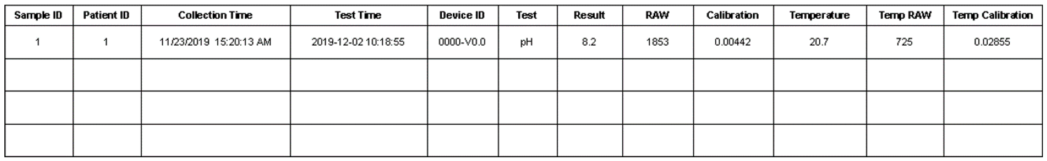
The samples table, shown in Figure 16, recorded each measurement of the specific sample from the patient. The measured data would be recorded from the hardware device directly. The temperature was always recorded with each measurement. The sample collection date and measurement time would be stored, too.

The brief description of each field in the database samples table is shown in

Table 1. Database samples table fields’ descriptions.

Field Name	Description
Sample ID	Index and primary key of table that defines each sample or measurement
Patient ID	Foreign key that links the patient to sample or test
Collection Time	Date and time that sample taken from patient
Test Time	Date and time (timestamp) of measurement
Device ID	Serial number and firmware version of device used for measurement
Test Type	The type of measurement includes pH, Ca2+, uric acid and conductivity The unit of measurement (UOM) is defined as part of this field
Result	The measured calibrated final value in the UOM defined in test type and after implementing the effect of temperature
RAW	The raw value measured by ADC before calibration factor applied
Calibration	The value multiplied by raw value to calibrate the result
Temperature Fields	Three fields are dedicated to temperature for result, raw data and calibration factor

.

2.4. Machine Learning Process

Basically, logistic regression is a typical supervised machine learning classification algorithm. It takes the features as input and calculates the probability that an observation belongs to a certain class by using a logistic function. The theoretical intuition behind this is the maximum likelihood estimation. Compared with other popular classification algorithms such as support vector machines (SVMs), whose classification results only rely on the support vectors, logistic regression is more robust to outliers, because all samples contribute to the classifier to maximize the likelihood. Additionally, logistic regression has the advantage of obtaining the classification probability, being easy to implement and having a low computational cost. However, all machine learning models have the problem of underfitting and overfitting (bias variance trade-off), so they can make mistakes. To solve this problem, we considered adding some regularization terms (L1 reg or L2 reg) to obtain good results in practice.

The desired output from the system was a binary result, whether the person was a potential stone-former or not. Although the data set from the test results generated by the system could be used with different model development techniques, logistics regression was selected for this work. Compared with other modeling approaches, logistics regression was more suitable for binary outputs. Four measured parameters in the urine sample of an individual along with age and gender formed the input vector. Figure 17 shows the input and output of the model.

In logistics regression modeling, the log odds of the output will be the linear combination of the inputs. Equation (6) shows the inputs as a vector column (vector X) with six elements:

$$\overline{X}=\left[\begin{array}{c}{x}_1\\ x_2\\ x_3\\ x_4\\ x_5\\ x_6\end{array}\right]\begin{array}{c}UricAcid\\ pH\\ C{a}^{2+}\\ Conductivity\\ Gender\\ Age\end{array}$$

(6)

where y is the output with a binary value. If the individual is a stone-former, the value of y = 1, and if the individual is not stone-former, y = 0. Then, as shown in Equation (7), the p(X) is the probability of an individual being a stone-former with the urine sample measurement results, gender and age defined by X:

$$p\left(\overline{X}\right)=prob\left(y=1|\overline{X}\right)$$

(7)

In the logistics regression model, the log odds of the output is a linear combination of the input, as in shown in Equation (8):

$$\ell =\log \frac{p\left(\overline{X}\right)}{1-p\left(\overline{X}\right)}={\beta }_0+{\beta }_1{x}_1+{\beta }_2{x}_2+{\beta }_3{x}_3+{\beta }_4{x}_4+{\beta }_5{x}_5+{\beta }_6{x}_6$$

(8)

In order to have a vector format while still accommodating the constant β₀, an element 1 will be added as the first row of vector X so it becomes a 7 × 1 vector. The goal of the training phase is to find the coefficient β for the maximum likelihood estimation. Equation (9) shows the relationship in vector format:

$$\overline{X}=\left[\begin{array}{c}1\\ x_1\\ x_2\\ x_3\\ x_4\\ x_5\\ x_6\end{array}\right],\overline{\beta }=\left[\begin{array}{c}{\beta }_0\\ {\beta }_1\\ {\beta }_2\\ {\beta }_3\\ {\beta }_4\\ {\beta }_5\\ {\beta }_6\end{array}\right],\log \frac{p\left(\overline{X}\right)}{1-p\left(\overline{X}\right)}={\overline{\beta }}^T\overline{X}\Rightarrow p\left(\overline{X}\right)=\frac{1}{1+e^{-{\overline{\beta }}^T\overline{X}}}$$

(9)

Using the gradient decent method, the coefficient β could be found by an iteration of Equation (10), while α is the learning rate and σ(x) is the sigmoid function:

$$\begin{array}{l}\sigma \left(x\right)=\frac{1}{1+e^{-x}}\\ {\overline{\beta }}^{new}=\overline{\beta }+\alpha {\displaystyle \sum _{i=1}^n\left[y_i-\sigma \left({\overline{\beta }}^T{\overline{X}}_i\right)\right]{\overline{X}}_i}\end{array}$$

(10)

The iteration would continue until β converged to the final value or until a certain number of iterations. In the testing phase and system operation as point-of-care, the p(X) would be calculated and compared with a threshold, typically 50%. If the p(X) became larger than the threshold, the urine sample under the test was from a potential stone-forming individual. Otherwise, the person had low risk to develop kidney stones.

2.5. Testing Materials and Instruments

The validation process was divided into three sections. The potentiometric readout circuit was tested using the commercial buffer solutions from Honeywell Fluka™ (Charlotte, NC, USA). Five buffer solutions—a Honeywell Fluka™ buffer solution of pH 4.0-citric acid/sodium hydroxide/sodium chloride solution with fungicide-, a buffer solution of pH 6.0-citric acid/sodium hydroxide solution with fungicide and traceable to Standard Reference Material (SRM) from National Institute of Standards and Technology (NIST)-, a buffer solution of pH 7.0-potassium dihydrogenphosphate/disodium hydrogen phosphate traceable to SRM from NIST with fungicide-, a buffer solution of pH 8.0-borax/hydrochloric acid, traceable to SRM from NIST- and a buffer solution of pH 10.0-borax/sodium hydroxide-—were used for testing the system. The pH-meter model LAQUAtwin pH-11, manufactured by Horiba Ltd. (Kyoto, Japan), was calibrated according to the manufacturer instructions and used for comparing the results of the test.

For validating the performance of the amperometric sensor readout circuit, we prepared several buffer solutions. The 500 ppm (parts per million) uric acid solution was made by mixing 100uL of a pH8.5 (0.1M) NaPB buffer with 50mg of uric acid powder. The 400 ppm uric acid solution was made by diluting 8 uL of a 500 ppm solution and 2 uL of buffer. In a similar approach, the 200 ppm solution was made as a result of the dilution of 4 uL of a 500 ppm solution with 6 uL of buffer. A solution of 100 ppm was made by diluting 2 uL of a 500 ppm solution with 8 uL of buffer. The electrochemical analyzer model CHI 600 E, manufactured by CH Instruments Inc (Austin, TX, USA),was used for validating the measured test results from the amperometric sensor readout circuit.

The performance of the conductivity readout circuit was validated using a commercial conductivity standard solution kit, model 503-S from Horiba Ltd. (Kyoto, Japan). The kit included potassium chloride (KCl) buffer solutions, with a conductivity range between 84 uS/cm and 111.8 mS/cm. The conductivity meter, model LAQUAtwin EC-33, manufactured by Horiba Ltd. (Kyoto, Japan) was used for comparing the results from the conductivity readout circuit.

3. Results and Discussion

The details of the chemical buffer solutions and instruments which were used for validating the system measurement results were discussed in Section 2.

Figure 18 shows the comparison of the measurement results between our system and the commercial conductivity measurement instrument. The Horiba^® EC-33 instrument and the KCl buffer solutions were used as a reference to evaluate the conductivity measurement.

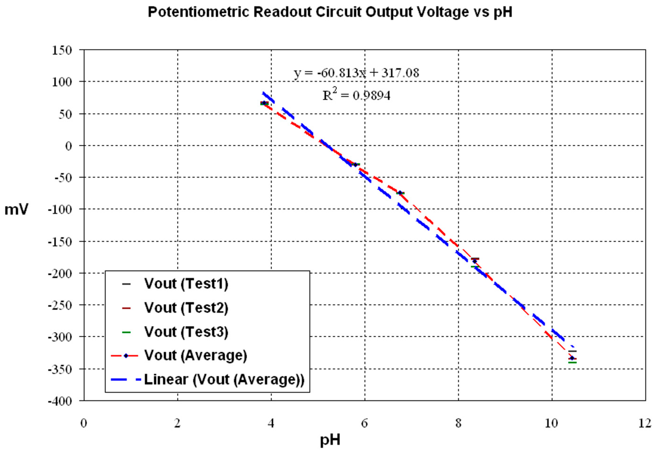
The potentiometric readout circuit was tested by measuring its output voltage and comparing it with the pH measurement from the commercial instrument, the Horiba^® pH-11. The Honeywell Fluka^® commercial buffer solutions were tested. The results curve is shown in Figure 19.

The uric acid concentration measurement had more complexity. A disposable sensor strip provided by Bioptik Technology Inc. was used for this measurement. A specific oxidation voltage should be provided for the sensor, and later the sample would be dropped on the strip. A sharp increase in current would be the time zero for the measurement. After a certain period of time, the measured current was proportional to the uric acid concentration in the sample.

The CH Instruments 600E electrochemical analyzer and the NaPB buffer solution were used for the comparison of measurements from the amperometric readout circuit. Figure 20 shows the sensor output current versus time. The measurement of the current was time-sensitive, as the sensor current increased sharply after dropping the sample and decayed exponentially.

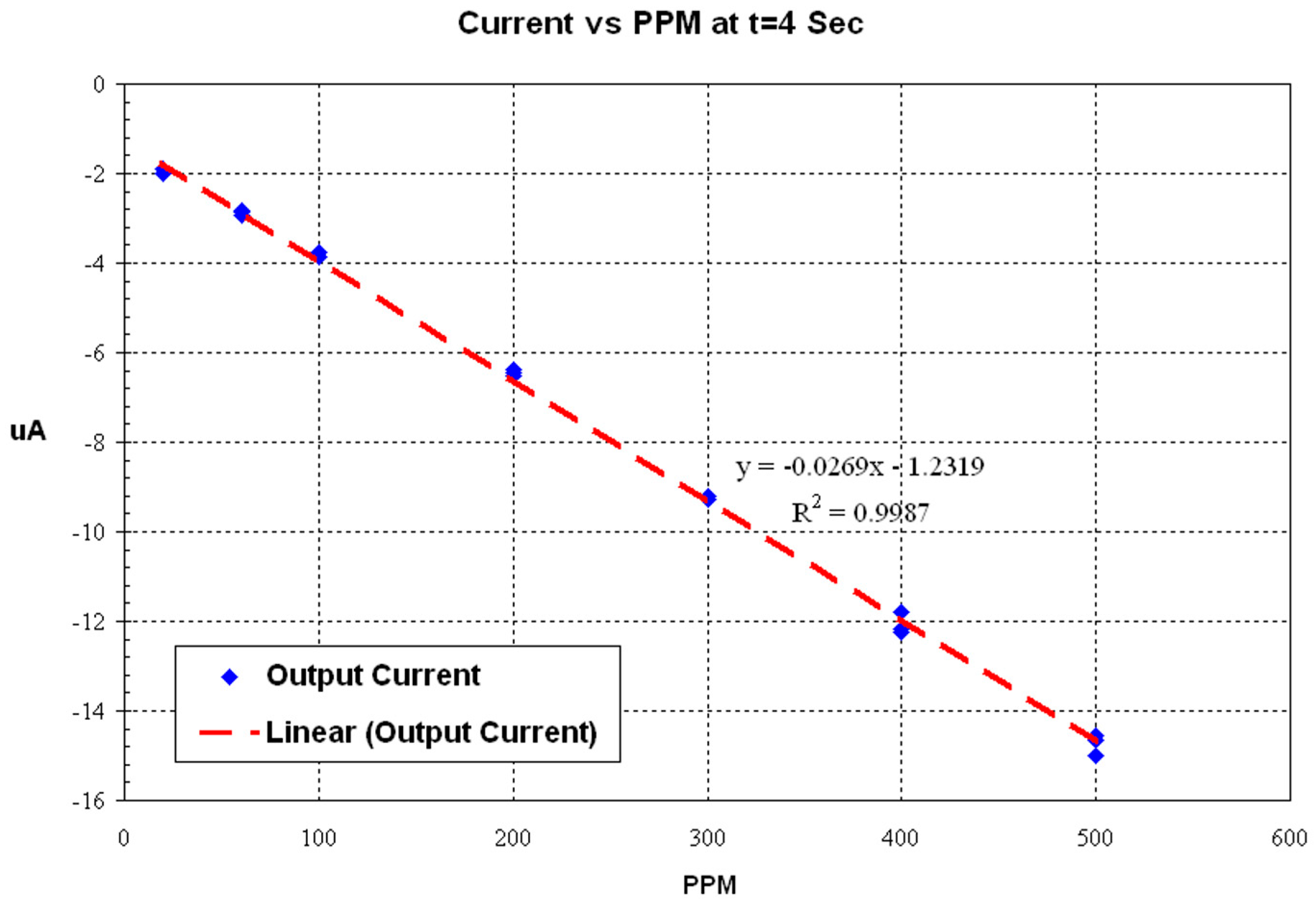
The sharp rise of the current considered the reference of time, and actual current measurement should be performed after a specific delay. The test results of measuring the sensor current 4 s after the time reference is shown in Figure 21. Uric acid buffer solutions were used for this test.

Table 2. Testing range of the system vs. typical human urine range.

Sensing Parameter	Sensing Range	Typical Human Urine	Capability to Be Used
pH	2–10	4.5–8	Yes
Ca2+	0.1–3.0 mmol/L	0.1–2.5 mmol/L	Yes
Uric Acid	20–500 ppm	<400 ppm	Yes
Conductivity	1–40 mS/cm	5–38 mS/cm	Yes

shows the summary of the testing range of the system compared with the typical human urine range for the same parameter. The last column shows if that parameter has the capability to be used as indicator for assessing the risk of forming kidney stones. In general, the system achieved a sensing range to accommodate the physiological range of such measurands in urine.

The next phase of our research is the utilization of actual urine samples collected from stone and non-stone formers. By using a multi-sensing approach in tandem with machine learning capability, we infer that we will achieve good correspondence with actual clinical diagnosis in the assessment of stone formation. Thus, our system can be a potent piece of technology for rapid screening and point-of-care testing application.

4. Conclusions

This paper presented the design and implementation of a multi-sensor platform for the measurement and data collection of four key parameters in urine samples to evaluate the risk of urolithiasis in its early stages. Verification with standard solutions has shown that our system correlates well with measurements from standard instruments. It also exhibited a sufficient sensing range to accommodate the physiological range in human urine. The fabricated on-board system will be distributed to different locations to collect the data. As a future work, the system design will be adapted for the development of low cost, low power consumption, compact on-chip application to be used as a point-of-care or personal care instrument.