Abstract
To reduce congestion, numerous routing solutions have been proposed for backbone networks, but how to select paths that stay consistently optimal for a long time in extremely congested situations, avoiding the unnecessary path reroutings, has not yet been investigated much. To solve that issue, a model that can measure the consistency of path latency difference is needed. In this paper, we make a humble step towards a consistent differential path latency model and by predicting base on that model, a metric Path Swap Indicator (PSI) is proposed. By learning the history latency of all optional paths, PSI is able to predict the onset of an obvious and steady channel deterioration and make the decision to switch paths. The effect of PSI is evaluated from the following aspects: (1) the consistency of the path selected, by measuring the time interval between PSI changes; (2) the accuracy of the channel congestion situation prediction; and (3) the improvement of the congestion situation. Experiments were carried out on a testbed using real-life Abilene traffic datasets collected at different times and locations. Results show that the proposed PSI can stay consistent for over 1000 s on average, and more than 3000 s at the longest in our experiment, while at the same time achieving a congestion situation improvement of more than 300% on average, and more than 200% at the least. It is evident that the proposed PSI metric is able to provide a consistent channel congestion prediction with satisfiable channel improvement at the same time. The results also demonstrate how different parameter values impact the result, both in terms of prediction consistency and the congestion improvement.
1. Introduction
The traffic in backbone networks has grown exponentially during the past two decades. With the ever-growing data-intensive applications relying on the Internet, the growth will be accelerated and the backbone networks will be increasingly overloaded. To adaptively select the optimal route for backbone network has been the main goal of research over decades [1,2,3,4,5,6,7]. However, as current routing strategies, such as OSPF, RIP, and EIGRP, use stationary channel measurement as criteria [8,9], it is difficult to predict an optimized route that will stay optimal for a long time when the channel congestion situation keeps oscillating, especially during peak hours [2,5,10,11,12,13,14]. Based on the criteria of the current routing strategy, the optimal route selected often changes frequently in extremely congested networks. When a path is congested due to large amount of traffic flows, the latency soars and the router swaps to another path, and after that, the traffic redirected to the backup path makes the path congested and its latency increase sharply, and now the original path seems to be the optimal one again, etc. Such reroutings are a huge waste to computation resources and energy power, and the rerouting delay may affect the quality of service (QoS) and user experience ultimately. Being able to reduce the number of reroutings by selecting a path that is consistently optimal over a relatively long time is thus important. How to model that a path is optimal over a long period of time so that it can work as a metric for the consistent optimal route is the question that we are trying to answer in this paper. Numerous solutions have been proposed for adaptive routing in backbone networks, but this question still exists in current telecommunication networks.
There are two main trends in the current adaptive routing for backbone networks, using software defined networking (SDN) and/or artificial intelligence. Deemed as the next generation networking, SDN was adopted by most of the recent work on adaptive routing, taking advantage of the centralized control strategy [5,6,15,16,17,18]. These works involve one or more centralized controllers in their design, collecting global knowledge of the network to achieve optimized QoS for the entire network. Artificial intelligence technologies, like machine learning, and especially deep learning and reinforcement learning, have been widely adopted in various aspects that need data to predict [5,6,17,18,19].
In this paper, a metric of consistent adaptive routing is proposed to improve load balancing and achieve consistent adaptive routing by analyzing real-life backbone traffic and predicting future congestion situations. More specifically, the following contributions are made:
- –
- A Differential Path Congestion Consistency Model is proposed to describe the latency variation between two paths.
- –
- Based on the model, a Path Swap Indicator (PSI) is proposed to predict the future latency changing trend. Relying on learning the latest congestion situation and predicting the onset of a long-term and consistent channel deterioration, the routing strategy is able to make a long-term effective decision on the path switching, i.e., to switch the path if and only if the target path’s condition will be better than the current one over a relatively long period of time.
- –
- Experiments on a testbed built by the Docker network were carried out to evaluate the proposed strategy. The results are presented and analyzed in detail.
2. State of Art
Traffic engineering has been intensively investigated as an indispensable solution for network load balance by selecting routes. As a traditional traffic engineering strategy, Equal-Cost Multi-Path (ECMP) is widely adopted by operators in all IGP protocols such as BGP, OSPF, and EIGRP, to spread traffic loads across multiple equal-cost (or unequal-cost, if manually configured so in EIGRP, which is the only protocol supporting unequal-cost multiple routes) routes available [20,21,22]. ECMP usually selects a path using flow hashing, queries, and weights. Widely adopted as it is, ECMP has many shortcomings that need to be addressed: (1) without a route congestion detection mechanism, ECMP may deteriorate the channel situation by sending flows to already congested routes. Additionally, hash collision may also increase the chances of channel congestion when using flow hash to select a path. (2) Without a global view of network topology, ECMP fails to provide optimized load balancing in unbalanced networks. (3) Unaware of flow sizes, ECMP is not able to recognize mouse flows and elephant flows, and thus performs poorly in load balancing when mouse flows and elephants flows co-exist (for example, it is not able to split the elephant flow into smaller ones and re-allocate).
Traditional traffic engineering strategies achieve optimal network performance by rerouting flows as often as possible whenever necessary, without considering the negative impacts. The consequent network instability, also referred to as route flapping, has been the interest of researchers in telecommunication networks since decades ago. Traditionally there are two main approaches to control route flapping: one is route dampening, which suppresses the flapped router by adding a penalty to it, and the other is route aggregation, also known as route summarization, which take multi-routes and clusters them into one inclusive route. These methodologies try to reduce route flapping passively; in other words, they do not change the flapping route itself, but execute some additional calculations and operations on these flapping routes instead. Thus, the effect of both methods are limited. In recent work, the necessity of global optimization and avoiding routing weight changes as much as possible was first addressed in [4], debriefing several reasons why routing weight changes are bad in networks, because: (1) even a single weight change can cause disruption in the network environment, for it needs to be flooded to all the routers, and then all the routers will have to recompute their optimal paths and communicate with each other to reach a global agreement. The whole process takes several seconds usually [4]. (2) When more than one weight change happen simultaneously, chaos will be caused throughout the network, and more time and bandwidth overhead will be consumed. (3) Human network operators are prone to overlook weight configurations until a concrete problem happens. In this paper, our proposed method takes the history latency of both the path and a competing path into consideration, and achieves more stability (gets a stable route that lasts for more than 3000 s at the longest and more than 1000 s on average) which is the main goal of route flapping reduction research.
Traditional traffic engineering strategies are made based on observation of current networks and configure routers to accommodate with the current situation only, which leaves the network unable to adapt to future traffic changes. Prediction-based traffic engineering has drawn interest in various domains by predicting future network traffic. The prediction time scale varies from milliseconds to seconds, minutes, days, weeks, or even months [23,24]. Artificial intelligence technologies, and especially machine learning, have drawn huge interest in prediction-based traffic engineering [5,6,17,18,19]. The essence of machine learning is to try to find the hidden pattern beneath history data, and use the pattern to predict the future. The models used to find the pattern can vary vastly, and there are hundreds of novel models proposed every year. However, it does not mean that the more complicated the model is the better; on the contrary, most of the time, less is more. It is the model that works most efficiently that best suits the pattern underneath history data. Additionally, current machine learning models require expensive hardware (like GPU) to run, and consume more time and computing resources than our proposed methodology, as presented in the following section.
3. Consistent Path Congestion Model
In this section, we propose a probabilistic model to describe the consistency of differential path congestion between two candidate route paths with the same source and destination nodes. Based on this model, the metric to evaluate the path congestion consistency is outlined.
Almost all existing approaches perform static network latency prediction based on the history values of round-trip times (RTTs), assuming the latencies are stable or unchanged, whereas in reality latencies can vary dramatically over time due to changing network conditions. Thus, among the state-of-art adaptive routing strategies using latency prediction, only a few could provide an approach to avoid the oscillation of route selection during peak hours.
3.1. Consistent Path Congestion Model and Its Related Algebra
Let paths i (the current path) and j (the backup path) be the two available paths between the same source and destination routers in a backbone network, and , are the latencies of the two paths, respectively, at time t. In this paper, we measure congestion with latency.
3.1.1. Differential Path Congestion Indicator
The situation that “the congestion of the current path is worse than the backup path to a certain degree” in continuous time is denoted by the Differential Path Congestion Indicator (DPCI) :
Whenever is 1, it means that at time t the latency of path i exceeds path j by more than seconds, as shown in Equation (2). Here the congestion is measured by latencies; thus , which is the Latency Differential Sensitivity, denotes a certain amount of congestion with a certain amount of latency.
Then is regarded as the output of a two-states continuous time random process. We name this underline process the Continuous-Time Differential Path Congestion Model (CDPCM) for Path i and j. It is worth mentioning that the does not preserve commutativity, that is:
For the convenience of analyzing, we need to transfer the continuous random process into a discrete one by sampling. When sampling at a sampling interval , we get a discrete random series ; n is integer and , which can be deemed as the output of a two-states discrete time random process. We name this process the Discrete Time Differential Path Congestion Model (DDPCM) for Path i and j. Similarly, does not preserve commutativity either, in other words,
3.1.2. Cumulative Differential Path Congestion Indicator
Based on the DPCI, the consistency of the relative path congestion situation can be modeled with the cumulative differential path congestion indicator (CDPCI) . is the frequency when the latency of path i exceeds path j by more than seconds during the recent period of time T. It describes the fact that “during the recent time period T, the situation that the congestion of the current path is worse than the backup path to a certain degree θ has happened times”. is derived from the sum of over the period of time T, based on the definition of DPCI , as shown below:
where T is the cumulative window, which is the time period of the history that is taken into consideration. Both and T are constant empirical values that are customer-configurable. In our experiment, the sampling intervals were s, s, and ms.
3.1.3. Cumulative Differential Path Congestion Consistency Indicator
To predict a stable high-volume traffic period, first we try to capture evidence that the CDPCI increases, which denotes “the situation that the congestion of the current path is worse than the backup path to a certain degree happens more/less often.”
We use the indicator to denote the process that increases/decreases comparing to the last value .
The Cumulative Differential Path Congestion Consistency Indicator (CDPCCI) is used to describe the situation that “the congestion of the current path is worse than the backup path to a certain degree more/less often, and the trend of increase/decrease has continued for more than a certain number of times during a recent time period”, denoted by “ keeps increasing/decreasing for more than a certain number of times during a recent certain time period”, which in turn can be described with Equations (8) and (9) as shown below, in which is the Latency Consistency Sensitivity, which represents the “number of times that has increased/decreased”, and is the Consistency Cumulative Window, which is the time period that is taken into consideration when measuring the CDPCCI.
The meanings of and are explained as follows. When , it means path j’s situation will be better than path i for the foreseeable future, and this situation will last longer than the route switching time consumption, which is less than 1 s in our experiment. The values of and have a strong impact on the performance of the indicator’s accuracy, and thus should not be too large or too small. If the value is too large, it means that the indicator stays equal to 0 (which means “stay in the current path”) even when the current channel’s situation is worse than the backup one, thus causing unnecessary congestion, delay, and further QoS deterioration. When is too small, by contrast, it may make the indicator too sensitive, jumping between the two paths with slight path latency jittering and causing routing oscillations. Similarly, when the value is set too high, the algorithm may fail to switch back to the original path when the backup path’s situation deteriorates and becomes more congested than the original one, causing QoS deterioration. When is too small, indicators will be too sensitive to the path’s latency changes and cause router flapping and network oscillation. The ideal threshold values are empirical facts, and may not be constant values. They depend on the real-time traffic on the paths in the network.
In our evaluation experiment, where the traffic data used were from real-life Abilene peak time traffic data, we found that the ideal values and or best indicate the situation of our experimental setup, as will be discussed in detail in Section 4.
3.2. Path Swap Indicator
The Path Swap Indicator (PSI) is defined in Table 1 as the indicator for differential path congestion consistency. In the following context, the parameters of CDPCCI are omitted where no ambiguity occurs.

Table 1.
Definition strategy of Path Swap Indicator at time .
Table 1 and the continuation of this section present in detail the derivation logic of the PSI , elaborating at each time t, how is determined from CDPCSI . When , it implies that it is necessary to switch the route to the backup path j, while means the route should stay with the current path i. From Table 1 and Equation (6) and (7), we can see that when is 1 and is 0, it implies that the latency on the current channel has exceeded the backup one and is still steeply increasing. This works as a sign that the current path’s situation will keep deteriorating in the near future, and thus it is worth to switch to the backup one. On the contrary, when is 0 and is 1, it indicates that the backup channel’s situation has worsened and will keep deteriorating in the near future, meaning we should stay with the current route. There is also a relatively rare case when both and are 1; it happens when both channels are experiencing serious turbulences. In this case, we chose to have indicator stay unchanged until there is an obvious and steady difference between the channels.
3.3. A Demo of the PSI Calculation Process
A step-by-step color-coded demonstration of how to get the proposed indicator PSI is given in Figure 1. In this demo, there are 21 data records, which is a fragment of the real-life traffic dataset. The parameters used in this demo are shown in Table 2. From Figure 1 it is obvious that the period when PSI (the red zone) starts as soon as the is 1 (the yellow zone), and ends when the first turns to 1 (the green zone).
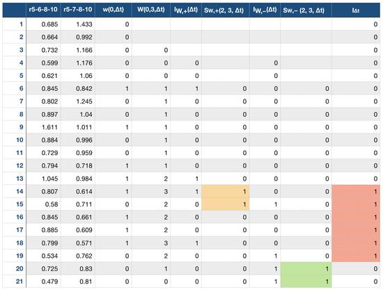
Figure 1.
A demo of the calculation process of each of the indicators proposed, on a sample of 21 data records obtained from an experiment with real-life Abilene Backbone network traffic data.
Table 2.
Parameters used in Experiment 2.
4. Evaluation
We evaluated the proposed strategy in a network constructed by the Docker network (https://www.docker.com), which has a topology that is the same as that of the Abilene network, as shown in Figure 2. We created real Docker networks as subnets, and imported Docker containers from image shtsai7/server as routers. Three different real-life Abilene backbone network traffic datasets were used as input traffic data. The baseline routing protocol was OSPF, which is the dominant intra-domain routing protocol. The network was simulated with Docker. Eleven Docker containers were created to simulate the eleven routers in the Abilene network. For each of the Docker containers, one Docker network was created for the Internet connection with the subnet name of 170.*.0.0/16. Fourteen Docker networks were created to simulate the connections between routers in the Abilene network, and they belonged to subnet 10.1.*.0/24. In each Docker container, Quagga https://www.quagga.net was used to configure OSPF in each router in the network.
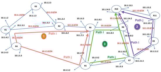
Figure 2.
Topology of the network of the evaluation experiment generated by a Docker network, which is the same as the real-life Abilene network.
The goal of this evaluation experiment is to attempt answering the following questions:
- Q1:
- Is the proposed PSI able to predict when one path’s situation is steadily better than the other (in terms of latency), in different extreme situations? In other words, how often is path i’s congestion situation indeed worse or better than path j (i.e., ) when their indicators are 1 and 0, respectively, and to what extent was the channel situation improved by the PSI indicator.
- Q2:
- How consistent is the predication, or in other words, what is the frequency of path swaps, or in yet another way to put it, how long does it last between the indicator swaps in extremely congested situations when the latency difference between paths oscillate.
To answer these two questions, the following metrics were used:
- –
- True/False rate, which means the rate when the PSI has correctly predicted the congestion situation between the current path and the backup path, including, when the PSI is 1, the latency of the current path is indeed larger than the backup one, and when PSI is 0, the latency of the current path is smaller than the backup one.
- –
- Latency difference, defined by the difference between the latency of the path selected by OSPF and the latency of the backup path , used as an indicator of the congestion comparison of the two paths. There are two main approaches to measure the latency: RTT, which is the time overhead for a packet to travel from source node to the destination and back, and Time for The First Byte (TTFB), which is the time overhead from the source to the destination node. In this paper, RTT is used like in most other works. As the latency testing tool, ping is used in this paper. Although there are some limitations of ping, (for example, ping works on ICMP packets but not TCP/UDP packets, and the former might have lower priority than the later in real-life backbone networks, and thus experience different latencies, which in turn results in inaccurate measurement), but in our experiment that was run on a Docker network simulated on one laptop, the ICMP and TCP/UDP packets shared the same priority; thus we argue that the latency difference is not an issue for the results demonstrated.
- –
- Accuracy improvement, which denotes when the PSI turns to 1, the increment in percentage of the times when the latency of the current path is indeed larger than that of the backup one.
- –
- Time interval between path swaps , which is the average time interval between PSI changes, as defined in Equation (10).
4.1. Dataset
Real-life Abilene network traffic data were used in the experiments [25,26]. The data from [25] are based on measurements of origin-destination flows taken continuously over a period of seven days, starting from 22 December 2003 to 29 December 2003. These data represent aggregate flow volumes for = 2016 consecutive 5 min time intervals over the week, across origin-destination pairs (including self-loops) of the 11 nodes of the Abilene network. The dataset from [26] is Abilene traffic measurements starting from 1 March 2004 to 10 September 2004 at 5 min time intervals. The datasets were cleaned and three sub-datasets with a period of 7 d each were selected randomly from them for the three experiments.
4.2. Experiment Setup
The software tools used in the experiment are listed below.
- -
- iperf (https://iperf.fr) A tool that actively measures the maximum achievable bandwidth.
- -
- ping (http://man7.org/linux/man-pages/man8/ping.8.html) A tool that uses the ICMP protocol to test whether a host is up or down, measuring Round-Trip Time (RTT) and packet loss statistics at the same time.
- -
- tc (http://www.man7.org/linux/man-pages/man8/tc.8.html) A linux shell command to show and manipulate traffic control settings.
- -
- quagga (https://www.quagga.net) A network routing software suite providing implementations of OSPF, Routing Information Protocol (RIP), Border Gateway Protocol (BGP), and IS-IS for Unix-like platforms, particularly Linux, Solaris, FreeBSD, and NetBSD.
To reproduce the extreme scenarios of a busy backbone network when peak traffic exceeds the channel bandwidth aggressively and thus deteriorates the channel QoS in terms of latency, we configured the bandwidth of each channel with the linux traffic control tool tc so that the peak traffic transmit rate was 7.5, 10, and 20 times the channel bandwidth. As tested by the Linux tool ping, the maximum transmit rate of the network was found to be 200 Mbits/s. Thus three experiments were carried out with the bandwidths configured to 10, 15, and 20 Mbits/s.
For the three experiments, we used three different parts of the Abilene network topology simulated by Docker. From each part, two routers were chosen as source and destination nodes, between which multiple possible paths are available (two paths are considered in this paper, for convenience), as shown in Figure 2. In the first experiment, as shown in the orange lines and labels in Figure 2, R4 and R6 were selected as source node and destination node, respectively. To simplify the problem, we considered two paths between R4 and R6 only, namely R4-5-6, which passes by R4, R5, and R6, and R4-1-2-6, passing by R4, R1, R2, and R6. The path R4-5-6 was the selected route by OSPF, and R4-1-2-6 was the backup path. In the second experiment, as shown in the green lines and labels in Figure 2, R5 and R10 were chosen as the source node and destination node, respectively, The path selected automatically by OSPF was R5-6-8-10 which passes by R5, R6, R8, and R10, and the backup path was R5-7-8-10, which passes by R5, R7, R8, and to R10. In the third experiment, as labeled with the color purple in Figure 2, the source and destination nodes were R7 and R10. The path selected automatically by OSPF was R7-8-10, and the backup path was thus R7-9-11-10.
Throughout each experiment, we had ping running on every hop (for example, in the first experiment, ping ran on hops R1-R2, R2-R6, R6-R5, R5-R4, and R4-R1), measuring the latency on every hop (In real-life telecommunication networks, the latency could not be directly represented by the value measured by ping, but here these two values are deemed as equal for brevity). At the beginning of the experiment, Quagga and OSPF were initiated on all of the nodes. From a randomly chosen point of time, a traffic stream generated from the real-life Abilene network traffic dataset was sent from the source node, through the path chosen by OSPF (for example, R4-5-6 in the first experiment). Then, after a random-length time period, another traffic stream generated by our traffic model was routed along the other path (e.g., R4-1-2-6 as in the first experiment). The latency of each path was calculated by summing up all of the latencies on every hop.
4.3. Results
Experiment results are shown in Figure 3, Figure 4, Figure 5, Figure 6, Figure 7 and Figure 8, and Table 3, Table 4, Table 5, Table 6 and Table 7. The parameters used in all the experiments are listed in Table 3. The PSIs calculated by the proposed method and the corresponding True/False rates are listed in Table 4, Table 5, Table 6 and Table 7, and their summaries are provided in Table 8 and Table 9. The effect of different values for parameter was also examined in the third experiment, as shown in Table 6 and Table 7 and Figure 5 and Figure 6.
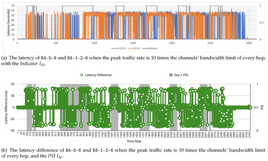
Figure 3.
The latency of OSPF chosen path and the backup path with the PSI under extreme cases of our pressure experiments. The peak traffic transmit rate is 10 times the channels’ bandwidth limit.
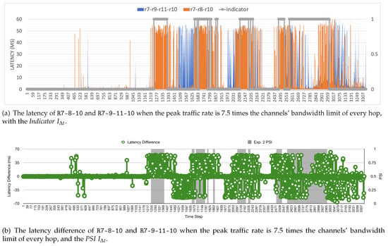
Figure 4.
The latency of the OSPF chosen path and the backup path with the PSI under extreme cases of our pressure experiments. The peak traffic transmit rate is 7.5 times the channels’ bandwidth limit.
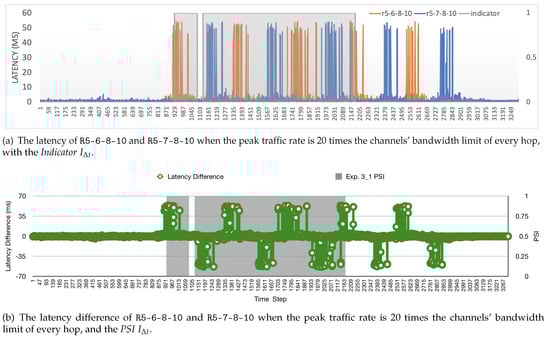
Figure 5.
The latency of the OSPF chosen path and the backup path with the PSI under extreme cases of our pressure experiments. The peak traffic transmit rate is 20 times the channels’ bandwidth limit.
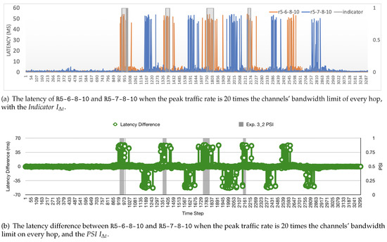
Figure 6.
The latency of the OSPF chosen path and the backup path with the PSI under extreme cases of our pressure experiments. The peak traffic transmit rate is 20 times the channels’ bandwidth limit.
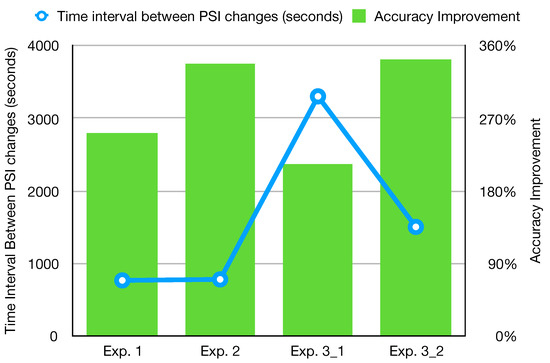
Figure 7.
The average time interval between PSI changes and accuracy improvement of each experiment.
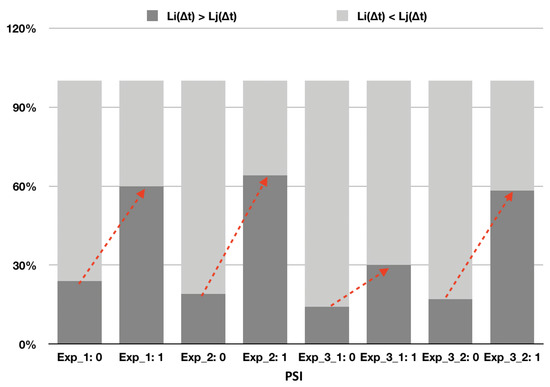
Figure 8.
Summarization and comparison of the accuracy improvement of each experiment.
Table 3.
Parameters used in all experiments.
Table 4.
Experiment 1’s evaluation result of proposed PSI between path R4-1-2-6 and path R4-5-6.
Table 5.
Experiment 2’s evaluation results of the proposed PSI between path R7-8-10 and path R7-9-11-10.
Table 6.
Experiment 3_1’s evaluation result of the proposed PSI between path R5-6-8-10 and path R5-7-8-10.
Table 7.
Experiment 3_2’s evaluation result of the proposed PSI between path R5-6-8-10 and path R5-7-8-10.
Table 8.
The accuracy result of all experiments with corresponding PSI.
Table 9.
Time intervals between swaps in all experiments.
4.3.1. Results of Experiment 1
Experiment 1 was carried out on the network denoted by orange and labelled with 1 in Figure 2. The source and destination routers were R4 and R6, respectively. The path chosen by OSPF was R4-5-6, as labelled with “Path i”, and the backup path was R4-1-2-6, labelled with “Path j”. The evaluation results are shown in Figure 3a,b and Table 4. In Figure 3a, the real-life latencies of both paths (R4-1-2-6 and R4-5-6) are presented with curves in orange (R4-5-6) and blue (R4-1-2-6) colors. As indicated before, the current path chosen by OSPF was R4-5-6, the orange curve in Figure 3a, and the blue curve is the latency of the backup path R4-1-2-6. The value of PSI at each time point is shown as a gray spot, and a continuous 1 s of indicator forms a window in Figure 3a. Inside the window the PSI is on, which means route should be switched to the backup path, and vice versa—outside the window the PSI is off, during which the route should be switched back to the current path, because it indicates that the current path has a better condition than the backup one according to our algorithm. The x-axis in Figure 3a is the number of steps of each measurement; each step is defined by the sampling interval , which was 5 s in this experiment.
In the ideal situation, when PSI is 1, the latency of the current path should always exceed the backup one, and vice visa. However, in the real-life backbone network, especially during busy hours when the traffic peak is 10 times the bandwidth, as in this experiment, the channel situation is very dynamic, and the congestion situation in terms of the latency difference will oscillate between two paths, as shown with the green line in Figure 3b; if we simply swap the route to the one with less latency, the router will be busy jumping back and forth between two paths, and the expense of rerouting will cause more than the channel improvement the rerouting brings. Thus, a consistent routing selection indicator is required. The metric to measure the consistency of the indicator selected in this paper is the time interval between path swaps ; the time interval can stay unchanged once the value of the indicator is set. As shown in Table 9, the indicator for route consistency is calculated as Equation (11).
Equation (11) implies that it is evident that, on average, each time there is a PSI change, it can stay consistent for 761.15 s. This is quite stable compared to the route change time expense, which is at the scale of milliseconds.
4.3.2. Results of Experiment 2
Experiment 2 was carried out on the topology labelled with purple and “2” in Figure 2. The source router was R7, and the destination router was R10. The path selected by OSPF was R7-8-10, and the backup one was R7-9-11-10. The evaluation results are shown in Figure 4a,b and Table 5, Table 8 and Table 9. In Figure 4a, the real-life latencies of paths (R7-8-10 and R7-9-11-10) are presented with curves in orange (R7-8-10) and blue (R7-9-11-10) colors. The latency of the current path chosen by OSPF R7-8-10 is denoted by the orange curve in Figure 4a, and the blue curve is the latency of the backup path R7-9-11-10. Same as in Experiment 1, the indicator at each time point is shown as a gray spot in Figure 4a. When the PSI is on (or has a value of 1), it indicates that the route should be switched to the backup path, because a steady increase of traffic load (or an elephant flow) in the current path is expected, and vice versa, when the PSI is off, it indicates the route should be switched back to the current path, because the current path has better conditions and will continue to stay better in a foreseeable future. The x-axis in Figure 4a is the step of each measurement, and each step is 5 s. The parameters chosen in the experiment are shown in Table 3.
in Experiment 2 is calculated in Equation (12), which means that on average, after a PSI change, it can stay consistent for 761.15 s. This is quite stable compared to the route change time expense, which is at the scale of milliseconds.
4.3.3. Results of Experiment 3
The third experiment was carried out on the topology labelled in green and “3” in Figure 2. The source and destination routers were R5 and R10, respectively. The evaluation result is shown in Figure 5a,b and Table 6, Table 8 and Table 9. In Figure 5a, the real-life latencies of paths (R5-7-8-10 and R5-6-8-10) are presented with curves in orange (R5-6-8-10) and blue (R5-7-8-10) colors. As indicated before, the current path chosen by OSPF is R5-6-8-10, the orange curve in Figure 5b, and the blue curve is the latency of the backup path R5-7-8-10. The indicator at each time point is shown as a gray spot in Figure 5a. The parameters chosen in the experiment are shown in Table 3.
As shown in Figure 5a, the PSI seems unable to reflect the channel changes. According to Table 8, when PSI = 1, only 30% of the latencies are really worse than the backup, and from Figure 7, the accuracy improvement of Experiment 3_1 is the lowest, only around . Thus we carried out another experiment, Experiment 3_2, adjusting the latency consistency sensitivity from 7 to 6, as shown in Table 3. The precision of the indicator has significantly improved, with the accuracy improvement raised to almost , as shown intuitively in Figure 6a,b and in Figure 7. It is evident that the experiment accuracy is very sensitive to the parameter latency consistency sensitivity , and thus customers should adjust it according to the real situation of their own network.
However, in Experiment 3_1, the time interval between path swaps was the highest of all experiments, as shown in Equation (13), which means that, after a PSI change, it can stay stable for 3303 s on average.
In Experiment 3_2, after the latency differential sensitivity was changed from 7 to 6, the time interval between path swaps decreased to 1500 s, as shown in Equation (14), but it was still 1500 times larger than the route change time, and thus it is evident that our proposed metric PSI is able to provide a consistent path congestion prediction.
4.3.4. Summary
The accuracy improvement and time interval between PSI changes of all experiments are summarized in Figure 7 and Figure 8 and Table 8 and Table 9. In Figure 8, each block represents the percentages of situations when the congestion in the backup path is better or worse than the current path (light gray denotes worse, and dark gray better). The red dashed arrow indicates the changing trend after the PWI turns to 1, and it is obvious that the smallest accuracy improvement is , while the largest improvement is almost , which evidences that the proposed PSI is able to relieve the congestion of the path by at least two and up to nearly four times. From Equations (11)–(14) and intuitively in Figure 7, it is also evident that each time the PSI changes its value, it can take effect for at least 760 s, and more than 3000 s at most. This is quite consistent compared to the route change time expense, which is less than 1 s according to technical reports of current vendors (https://docs.oracle.com/cd/E19934-01/html/E21707/z40004761412103.html https://www.cisco.com/c/en/us/support/docs/ip/open-shortest-path-first-ospf/7039-1.html#t6.)
The efficiency and consistency of the PSI are further presented in Figure 3b, Figure 4b, Figure 5b, Figure 6b, by putting the value of the PSI at each time step against the latency difference between the OSPF selected path and the backup one. In Figure 3b, Figure 4b, Figure 5b, Figure 6b, the green dotted lines are the differences between the latency of the chosen path and the backup path. The grey lines denote the values of the PSI at each time step. When the green dot is above 0, the OSPF chosen path is more congested than the backup path; when below 0, the backup path has a better channel situation. In these experiments, the peak traffic rates have exceeded the bandwidth by far (up to 20 times the bandwidth); thus during busy hours, the latency difference can be as large as milliseconds.
As suggested intuitively from Figure 3b, Figure 4b, Figure 5b, Figure 6b, the latency differences are dynamic and vibrating. This deduction can also be proved by the variances of latency differences, according to Table 9, in these experiments, the largest variance of latency difference reaches , while the consistency of the PSI can still be as high as 761.5 s, with a channel improvement of 251%. As for the traffic with the smallest variance 12.16, the PSI can stay unchanged for as long as 1500 s, while still achieving a congestion improvement of 342.9%, as denoted in Table 8.
In summary, we argue that it is evident that the metric PSI proposed in this paper is able to predict the path situation with acceptable precision and considerable consistency during extremely congested situations. Routing algorithms guided by this metric can achieve satisfiable improvement in the path congestion. It is worth mentioning that the prediction result is very sensitive to the parameters, especially Latency Consistency Sensitivity, that even small changes can affect the results significantly, and that parameters are dependent on the real network. Thus users should carefully chose their parameters according to their own network.
5. Conclusions
In this paper, an effort towards consistent adaptive routing in backbone networks under extreme congested conditions was proposed, with the main goal to avoid unnecessary path rerouting and reduce consequent network fluctuation and channel deterioration, by predicting the onset of an obvious and steady relative channel deterioration compared to the backup path. First we proposed a model to describe the differential channel congestion between the selected path and the backup one. Then, a metric for consistent routing, PSI, was designed, which is a boolean indicator for rerouting between the current path and the backup one. When the PSI is on, , it denotes that the backup path has and will have steady superior performance compared to the current path; thus it works as a sign to reroute traffic to the backup path. When the PSI is off, it denotes a steady inferior performance compared to the backup path.
Evaluation experiments have been carried out on real networks virtualized with the Docker network, using real-life Abilene network traffic datasets. Results were presented and analyzed in detail. It is evident from the results that the PSI is able to predict the trend of channel congestion consistently; once PSI changes, it will take effect for more than 1000 s on average and more than 3000 s at most, while improving the congestion situation by more than 300% on average. The parameter selection was also discussed: different parameter values were used and their effects were compared. It turns out that the design of the PSI is flexible with configurable parameters. For future work, the effect of the PSI will be further evaluated by implementing it in real-life backbone networks with various, and its effects in terms of metrics like the call block probabilities will be studied to compare with existing approaches.
Author Contributions
Conceptualization, D.P. and Q.Z.; methodology, Q.Z.; software, Q.Z.; validation, Q.Z.; formal analysis, Q.Z.; investigation, Q.Z. and D.P.; resources, Q.Z. and D.P.; data curation, Q.Z. and D.P.; writing—original draft preparation, Q.Z.; writing—review and editing, D.P.; visualization, Q.Z.; supervision, D.P.; project administration, D.P.; funding acquisition, D.P. All authors have read and agreed to the published version of the manuscript.
Funding
This research was supported in part by the UK Engineering and Physical Sciences Research Council (EPSRC) projects EP/N033957/1, and EP/P004024/1; by the European Cooperation in Science and Technology (COST) Action CA 15127: RECODIS—Resilient communication and services; by the EU H2020 GNFUV Project RAWFIE-OC2-EXPSCI (Grant No. 645220), under the EC FIRE+ initiative; and by the Huawei Innovation Research Program (Grant No. 300952).
Conflicts of Interest
The authors declare no conflict of interest.
Abbreviations
The following abbreviations are used in this manuscript:
| Latency of the Path i at time t | |
| Latency of the Path j at time t | |
| Latency Differential Sensitivity represent a certain amount of congestion by a certain amount of latency. | |
| Sample Interval | |
| T | Cumulative Window the time period of the history in step of that is taken into consideration when calculating . |
| Differential Path Congestion Indicator (DPCI) | |
| Discrete Time Differential Path Congestion Indicator obtained from by sampling at a sampling interval . | |
| Cumulative Differential Path Congestion Indicator (CDPCI) obtained from from the sum of over the period of time T. | |
| the process in which increases compared to the last value | |
| the process in which decreases compared to the last value | |
| Latency Consistency Sensitivity the number of times that has increased | |
| Latency Consistency Sensitivity the number of times that has decreased | |
| Consistency Cumulative Window the time period that is taken into consideration when measuring path congestion consistency CDPCCI. | |
| Cumulative differential path congestion consistency indicator (CDPCCI) represents the situation in which keeps increasing for more than a certain number of times during a recent time period. | |
| Cumulative differential path congestion consistency indicator (CDPCCI) represents the situation in which keeps decreasing for more than a certain number of times during a recent time period. | |
| PSI derived from the CDPCCI indicators proposed. |
References
- Shaikh, A.; Rexford, J.; Shin, K.G. Load-sensitive routing of long-lived IP flows. ACM SIGCOMM Comput. Commun. Rev. 1999, 29, 215–226. [Google Scholar] [CrossRef]
- Zhang, J.; Ye, M.; Guo, Z.; Yen, C.Y.; Chao, H.J. CFR-RL: Traffic Engineering with Reinforcement Learning in SDN. arXiv 2020, arXiv:2004.11986. [Google Scholar] [CrossRef]
- Kandula, S.; Katabi, D.; Davie, B.; Charny, A. Walking the tightrope: Responsive yet stable traffic engineering. ACM SIGCOMM Comput. Commun. Rev. 2005, 35, 253–264. [Google Scholar] [CrossRef]
- Fortz, B.; Thorup, M. Optimizing OSPF/IS-IS weights in a changing world. IEEE J. Sel. Areas Commun. 2002, 20, 756–767. [Google Scholar] [CrossRef]
- Thomas, S.; Thomaskutty, M. Congestion bottleneck avoid routing in wireless sensor networks. Int. J. Electr. Comput. Eng. 2019, 9, 2099–8708. [Google Scholar] [CrossRef]
- Shih-Chun, L.; Akyildiz, I.F.; Pu, W.; Min, L. QoS-aware adaptive routing in multi-layer hierarchical software defined networks: A reinforcement learning approach. In Proceedings of the 2016 IEEE International Conference on Services Computing (SCC), San Francisco, CA, USA, 27 June–2 July 2016; pp. 25–33. [Google Scholar]
- Azzouni, A.; Boutaba, R.; Pujolle, G. NeuRoute: Predictive dynamic routing for software-defined networks. In Proceedings of the 2017 13th International Conference on Network and Service Management (CNSM), Tokyo, Japan, 26–30 November 2017; pp. 1–6. [Google Scholar]
- Moy, J. OSPF Version 2. Technical Report; RFC 2328. 1997. Available online: https://tools.ietf.org/html/rfc2328 (accessed on 23 July 1997).
- Albrightson, R.; Garcia-Luna-Aceves, J.J.; Boyle, J. EIGRP–A Fast Routing Protocol Based on Distance Vectors. In UC Santa Cruz Previously Published Works; 1994; Available online: https://www.ida.liu.se/~TDTS02/papers/eigrp.pdf (accessed on 23 July 1994).
- Yang, Y.; Wang, J. Design guidelines for routing metrics in multihop wireless networks. In Proceedings of the IEEE INFOCOM 2008-The 27th Conference on Computer Communications, Phoenix, AZ, USA, 13–18 April 2008; pp. 1615–1623. [Google Scholar]
- Kamat, P.; Zhang, Y.; Trappe, W.; Ozturk, C. Enhancing source-location privacy in sensor network routing. In Proceedings of the 25th IEEE International Conference on Distributed Computing Systems (ICDCS’05), Columbus, OH, USA, 6–10 June 2005; pp. 599–608. [Google Scholar]
- Ullah, R.; Yasir, F.; Byung-Seo, K. Energy and congestion-aware routing metric for smart grid AMI networks in smart city. IEEE Access 2017, 5, 13799–13810. [Google Scholar] [CrossRef]
- Rajesh, M.; Gnanasekar, J.M. Congestion Control Scheme for Heterogeneous Wireless Ad Hoc Networks Using Self-Adjust Hybrid Model. Int. J. Pure Appl. Math. 2017, 116, 519–536. [Google Scholar]
- Boroojeni, K.G.; Amini, M.H.; Iyengar, S.S.; Rahmani, M.; Pardalos, P.M. An economic dispatch algorithm for congestion management of smart power networks. Energy Syst. 2017, 8, 643–667. [Google Scholar] [CrossRef]
- Ranjana, P.; Jeevani, D.; George, A. Optimized Raco-Car Based Adaptive Routing in Mesh Network. Middle East J. Sci. Res. 2016, 24, 10–14. [Google Scholar]
- Kim, S.; Son, J.; Talukder, A.; Hong, C.S. Congestion prevention mechanism based on Q-leaning for efficient routing in SDN. In Proceedings of the 2016 International Conference on Information Networking (ICOIN), Kota Kinabalu, Malaysia, 13–15 January 2016; pp. 124–128. [Google Scholar]
- Yu, C.; Zhang, Z. Painting on placement: Forecasting routing congestion using conditional generative adversarial nets. In Proceedings of the 56th Annual Design Automation Conference, Las Vegas, NV, USA, 2–6 June 2019; pp. 1–6. [Google Scholar]
- Raman, C.J.; James, V. FCC: Fast congestion control scheme for wireless sensor networks using hybrid optimal routing algorithm. Clust. Comput. 2019, 22, 12701–12711. [Google Scholar] [CrossRef]
- Khatouni, A.S.; Soro, F.; Giordano, D. A Machine Learning Application for Latency Prediction in Operational 4G Networks. In Proceedings of the 2019 IFIP/IEEE Symposium on Integrated Network and Service Management (IM), Arlington, VA, USA, 8–12 April 2019; pp. 71–74. [Google Scholar]
- Elwalid, A.; Jin, C.; Low, S.; Widjaja, I. MATE: MPLS adaptive traffic engineering. In Proceedings of the IEEE INFOCOM 2001, Conference on Computer Communications, Twentieth Annual Joint Conference of the IEEE Computer and Communications Society (Cat. No. 01CH37213), Anchorage, AK, USA, 22–26 April 2001; Volume 3, pp. 1300–1309. [Google Scholar]
- Kar, K.; Kodialam, M.; Lakshman, T.V. Minimum interference routing of bandwidth guaranteed tunnels with MPLS traffic engineering applications. IEEE J. Sel. Areas Commun. 2000, 18, 2566–2579. [Google Scholar] [CrossRef]
- Srivastava, S.; Medhi, D. Traffic Engineering of MPLS Backbone Networks in the Presence of Heterogeneous Streams. Comput. Netw. 2009, 53, 2688–2702. [Google Scholar] [CrossRef]
- Papagiannaki, K.; Taft, N.; Zhang, Z.; Diot, C. Long-term forecasting of Internet backbone traffic: Observations and initial models. In Proceedings of the IEEE INFOCOM 2003. Twenty-second Annual Joint Conference of the IEEE Computer and Communications Societies (IEEE Cat. No. 03CH37428), San Francisco, CA, USA, 30 March–3 April 2003; Volume 2, pp. 1178–1188. [Google Scholar]
- Krithikaivasan, B.; Zeng, Y.; Deka, K.; Medhi, D. ARCH-Based Traffic Forecasting and Dynamic Bandwidth Provisioning for Periodically Measured Nonstationary Traffic. IEEE/ACM Trans. Netw. 2007, 15, 683–696. [Google Scholar] [CrossRef]
- Lakhina, A.; Papagiannaki, K.; Crovella, M.; Diot, C.; Kolaczyk, E.D.; Taft, N. Structural analysis of network traffic flows. In Proceedings of the Joint International Conference on Measurement and Modeling of Computer Systems, New York, NY, USA, 12–16 June 2004; Volume 32, pp. 61–72. [Google Scholar]
- Zhang, Y.; Roughan, M.; Duffield, N.; Greenberg, A. Fast accurate computation of large-scale IP traffic matrices from link loads. ACM SIGMETRICS Perform. Eval. Rev. 2003, 31, 206–217. [Google Scholar] [CrossRef]
Publisher’s Note: MDPI stays neutral with regard to jurisdictional claims in published maps and institutional affiliations. |
© 2020 by the authors. Licensee MDPI, Basel, Switzerland. This article is an open access article distributed under the terms and conditions of the Creative Commons Attribution (CC BY) license (http://creativecommons.org/licenses/by/4.0/).