Article

Audio-Based Aircraft Detection System for Safe RPAS BVLOS Operations

by
Jorge Mariscal-Harana
1,2,*,
Víctor Alarcón
1,*,
Fidel González
1,
Juan José Calvente
3,
Francisco Javier Pérez-Grau
1,
Antidio Viguria
1 and
Aníbal Ollero
4
1
Avionics and Systems, Advanced Center for Aerospace Technologies (FADA-CATEC), 41309 Sevilla, Spain
2
Department of Biomedical Engineering, School of Biomedical Engineering and Imaging Sciences, King’s College London, London SE1 7EH, UK
3
RPAS, Aertec Solutions, 41309 Sevilla, Spain
4
Robotics, Vision and Control Group (GRVC), University of Seville, 41092 Seville, Spain
*
Authors to whom correspondence should be addressed.
Electronics 2020, 9(12), 2076; https://doi.org/10.3390/electronics9122076
Submission received: 15 October 2020 / Revised: 1 December 2020 / Accepted: 3 December 2020 / Published: 5 December 2020
(This article belongs to the Special Issue Deep Learning Technologies for Machine Vision and Audition)

Abstract

:
For the Remotely Piloted Aircraft Systems (RPAS) market to continue its current growth rate, cost-effective ‘Detect and Avoid’ systems that enable safe beyond visual line of sight (BVLOS) operations are critical. We propose an audio-based ‘Detect and Avoid’ system, composed of microphones and an embedded computer, which performs real-time inferences using a sound event detection (SED) deep learning model. Two state-of-the-art SED models, YAMNet and VGGish, are fine-tuned using our dataset of aircraft sounds and their performances are compared for a wide range of configurations. YAMNet, whose MobileNet architecture is designed for embedded applications, outperformed VGGish both in terms of aircraft detection and computational performance. YAMNet’s optimal configuration, with >70% true positive rate and precision, results from combining data augmentation and undersampling with the highest available inference frequency (i.e., 10 Hz). While our proposed ‘Detect and Avoid’ system already allows the detection of small aircraft from sound in real time, additional testing using multiple aircraft types is required. Finally, a larger training dataset, sensor fusion, or remote computations on cloud-based services could further improve system performance.

1. Introduction

1.1. Motivation

Over the last years, the market for Remotely Piloted Aircraft Systems (RPAS) has grown exponentially. Given the increasing number of operators, the market for professional RPAS is estimated to exceed €10 billion in Europe by 2035 and generate more than 100,000 jobs, according to the SESAR’s European Drones Outlook Study [1].
One of the key points to reach this potential market is the transition from operations within visual line of sight to beyond visual line of sight (BVLOS), which offer a much higher added value. In fact, SESAR estimates that approximately 50% of the professional market will focus on BVLOS operations in rural environments for applications such as linear infrastructure inspection and monitoring, precision agriculture, and surveillance. In these kinds of applications, aerial platforms fly at a Very Low Level (VLL), a term which implies flight below 150 m.
When it comes to performing BVLOS flights in rural environments, the main roadblock is the absence of cost-effective ‘Detect and Avoid’ systems approved by the aeronautical authorities. These systems must ensure the absence of other aircraft, especially those flying at high speeds at VLL and which are part of the so-called ’non-collaborative traffic‘, i.e., any air vehicle that does not provide its position and whose detection depends only on ground-based systems.
Therefore, the two key aspects which highlight the relevance of this study are the recent changes in RPAS regulation [2] and the need to unblock their potential market in the short term with cost-effective technological developments, for the successful integration of their operations into non-segregated airspace.
One of the particularities of RPAS is the fact that the pilot is not on board the aircraft, losing the ability to directly detect other manned aircraft or RPAS. Thus, the concept of a ‘Detect and Avoid’ system for RPAS is introduced, which refers to the integration of sensors that allow the RPAS to recognize the environment and to navigate safely avoiding encounters and potential collisions. This problem is divided into two parts: the detection of objects around the aerial vehicle, and the management of the path followed by the RPAS so that collisions do not occur. This paper focuses on the first part of such a problem.

1.2. Related Work

This ‘Detect and Avoid’ concept has been the subject of research in recent years [3], but a standardized system for light RPAS has not yet been achieved. Current approaches involve large aerial vehicles which carry complex sensors and heavy computer systems, and which operate under Visual Flight Rules or Instrumental Flight Rules [4]. However, the requirements for such approaches differ considerably from those of RPAS in VLL operations. Other solutions that help increase the pilot’s ability to detect other aircraft are based on existing surveillance technologies such as Automatic Dependent Surveillance-Broadcast (ADS-B). ADS-B uses transponders to broadcast information to other airspace users such as their identifier, route, position, speed, etc. The main disadvantages are the security vulnerabilities and the need to mount an ADS-B transponder on the aircraft—which is not mandatory for general aviation or sport aircraft—making it not 100% reliable as a ‘Detect and Avoid’ system in VLL flights [5].
Although sensors for ’Detect and Avoid‘ systems are commonly placed on board the aerial platform (e.g., radar, visual cameras, ultrasonic, or laser), there are also systems which rely on ground-based infrastructure. These systems limit the operational area of the RPAS, but they have the advantage of reducing the aerial platform payload and the computational requirements on board and are especially suitable for VLL operations. Regarding ground-based technology, one development uses a Passive Secondary Surveillance Radar for aircraft surveillance [6], but their high cost limits their adoption in most use cases. Another ground-based approach proposes combining Kalman filtering and sensor fusion applied to video and acoustic vector sensor data for propeller aircraft detection and tracking [7]. Although this system achieves state-of-the-art detection accuracy (Q1 = 66%, Q2 = 77%, Q3 = 92%), it does so at distances <300 m and the author states an upper-detection limit of 1000 m. More recently, a drone detection system using LIDAR technology has been proposed, although its range is limited to a few hundred meters [8].
The current work is part of a larger project whose aim is to overcome the aforementioned limitations through the development of a ground-based ‘Detect and Avoid’ system. Its main goal is the early detection of manned aircraft within a two-kilometer radius, by combining images and audio acquired using low-cost sensors (cameras and microphones, respectively), advanced processing capabilities, and deep learning methods to preserve safety in BVLOS operations of RPAS.
Regarding the detection from images, the main challenges are the angle of view and the image resolution provided by low-cost cameras [9,10], since aircraft appear within just a few pixels for distances greater than two kilometers, as shown in Figure 1.
Regarding the detection from audio, the two-kilometer range is also an important aspect. However, the main challenges are the real-time detection of aircraft sounds and the avoidance of false positives from surrounding and closer sounds, such as those produced by ground vehicles.
The task of determining the source of a sound is known as Sound Event Detection (SED). Although conventional machine learning algorithms have been used for SED in the past, current state-of-the-art approaches are based on deep learning models [11,12]. Over the last years, deep learning algorithms have consistently outperformed conventional machine learning ones in the annual Detection and Classification of Acoustic Scenes and Events (DCASE) challenge [11]. In fact, most DCASE 2020 competitors used deep learning models based on convolutional neural networks (CNN), recurrent neural networks (RNN), or a combination of both, with the top performer achieving an F-score of 50% for SED in domestic environments [13].
Hershey et al. [14] compared the performance of several CNN architectures using the AudioSet dataset [15], which contains 5.24 million hours of labeled sounds (extracted from YouTube videos) corresponding to 632 different sound classes. The compared models were AlexNet [16], VGG (configuration E) [17], Inceptionv3 [18], and ResNet-50 [19]. Although they were originally designed for image classification, their SED performance was similarly outstanding, with ResNet-50 achieving an Area Under the Curve (AUC) value of 0.926. Alternative approaches have achieved state-of-the-art performance using either RNNs [20], a combination of CNN and RNN architectures [21], or Transformers [22]. Consequently, SED using deep learning has a number of current and potential applications, including road surveillance [23], human activity monitoring [24], music genre recognition [25], smart wearables and hearables, health care, and autonomous navigation [12].
Both approaches within this project—detection via image and audio—use supervised deep learning techniques to ensure the robustness of the aircraft detection system. Subsequently, sensor fusion techniques combining audio- and image-based predictions are applied with the aim of further increasing the robustness of the system to meet future requirements of ‘Detect and Avoid’ systems demanded by the authorities.
The aim of this paper is the development of an audio-based ’Detect and Avoid‘ system for small aircraft using CNN models trained on our dataset of aircraft sounds. Our contributions to the field of SED are the design and implementation of an embedded real-time aircraft detection system, and a comparison between state-of-the-art deep learning models for SED.
The remainder of the paper is organized as follows. In Section 2, we describe the proposed detection system, the dataset of aircraft sounds, and the SED models. In Section 3, we compare the performance and computational requirements of each model and discuss the implications of such results. Finally, in Section 4, we present the main conclusions of the study and make some recommendations for future research.

2. Materials and Methods

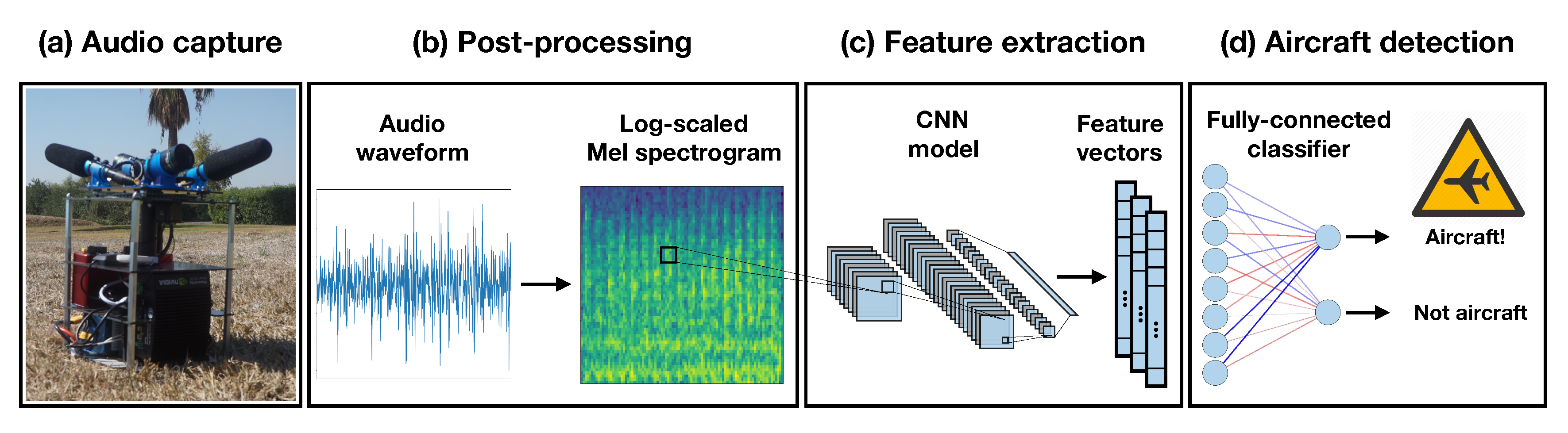
2.1. Aircraft Detection System

The aircraft detection system, whose task is to detect small aircraft within a two-kilometer radius, must run on a single self-contained, portable, embedded computer with a GPU that is powerful enough to run real-time inferences using deep learning models.
The system is composed of microphones, cameras, and an embedded computer, as shown in Figure 2a. The main sensors are two 20 megapixel RGB cameras (Basler acA5472-17uc with 25 mm Fujinon CF25ZA-1S lens) for image capture, and two directional microphones (Audio-Technica AT875R) connected to a two-channel audio card (Focusrite Scarlett 2i2) for audio capture. The addition of a servo motor allows a 360-degree rotation around the horizontal plane, which enables the cameras and microphones to cover the entire area around the ‘Detect and Avoid’ system. The embedded computer where both image and audio data are acquired and analyzed is an Nvidia Jetson TX2, and the real-time inferences are sent to a ground control station via a 4G connection provided by a USB network card. The current study focuses on the audio-based detection aspects of the system, which includes recording audio through the microphones and performing real-time inferences within the embedded computer to determine the presence or absence of nearby aircraft. A detailed description of the Nvidia Jetson TX2 configuration and model implementations is provided in Appendix A.
Figure 2 shows a summary of the audio-based ‘Detect and Avoid’ processing pipeline. First, audio signals are captured in real-time through the microphones (a). Then, the audio waveform is transformed into log-scaled Mel spectrograms (b), which are in turn fed into the pre-trained CNN model for feature extraction (c). Finally, a fully connected classifier determines if the sound belongs to an aircraft or not (d).

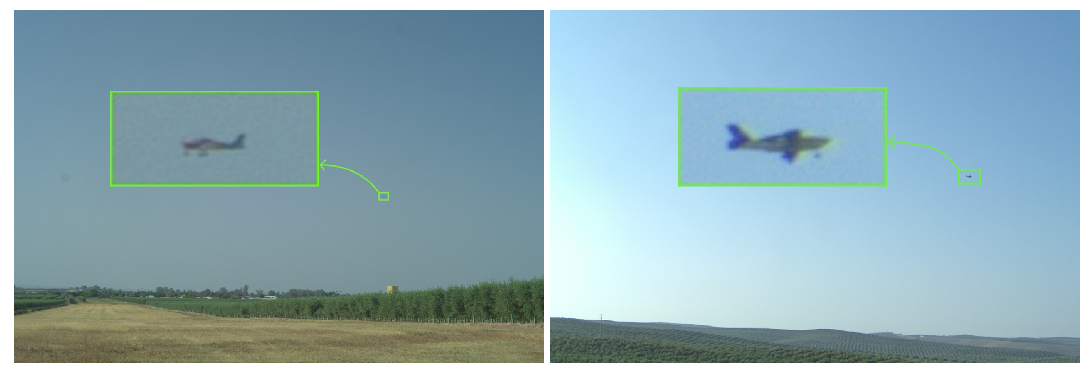
2.2. Dataset: Small Aircraft Sounds

The large amounts of data required to train deep learning models have motivated the creation of a number of datasets containing sounds from urban [27,28,29], domestic [30], industrial [31,32], and generic [15,33,34,35] environments. Nevertheless, sounds for our application are scarce and difficult to produce, given the particular focus of our ‘Detect and Avoid’ system: small aircraft flying at VLL and within two kilometers of the microphones.
In order to fine-tune existing SED models, we have curated a dataset of small aircraft sounds (‘Small Aircraft’ dataset) representing the ‘aircraft’ class. These audios were initially collected from free online audio databases, directly accessible through their websites [36,37,38]. However, since there were not enough available external data to successfully train our models, a data acquisition campaign was performed at ATLAS (Air Traffic Laboratory for Advanced Unmanned Systems) [39]. ATLAS is a test flight center located in Villacarrillo (Jaén, Spain), which is ideally suited for the development of experimental flights with unmanned aerial vehicles. The data acquisition campaign, consisting of a flight plan simulating a realistic scenario according to the objectives of the ‘Detect and Avoid’ system, took place in September 2019. A SOCATA TB9 aircraft executed a circular trajectory around the airfield runway, flying at an altitude between 90 m and 230 m, and at a distance between 1000 m and 2250 m from the aircraft detection system. With excellent weather conditions (i.e., light wind, few clouds, and high illumination), the aircraft was able to complete 11 laps.
Given that the human ear can detect air variations between 20 Hz and 20,000 Hz [40] that most aircraft sounds are located in the range from 10 Hz to 250 Hz [41], and that the selected neural network is limited to frequencies lower than 7.5 kHz, labeling was performed by a human operator. The exclusion criteria were the lack of clear aircraft sounds, the presence of excessive noise, the presence of multiple sounds together with aircraft sounds, and the type of aircraft sound (i.e., jet or large aircraft sounds were excluded). After manual labeling, the combined duration of aircraft sounds from free online sources (used for training) and from ATLAS (used for testing) was 0.6 h.
Additionally, the ‘UrbanSound8K’ dataset [27], which contains more than 8000 urban sounds (<4 s) originally divided into 10 sound classes, has been used to represent the ‘not aircraft’ class, with a total duration of 8.75 h. We choose this dataset since it contains a number of sounds (i.e., ‘drilling’, ‘engine idling’, ‘jackhammer’, and ‘air conditioner’) which are likely to produce false aircraft detections in rural environments.
However, due to the large difference in total duration between both datasets, we face the problem of class imbalance, where the minority class (i.e., ‘aircraft’) contains a much lower number of samples (i.e., feature vectors) than the majority class (i.e., ‘not aircraft’), as seen in Table 1. To overcome this problem, we follow four different strategies for the training data. Firstly, we undersample the ‘not aircraft’ class by randomly eliminating samples so that the size of both classes matches. We refer to the resulting dataset as the ‘Undersampling’ dataset. Secondly, we apply augmentation to the ‘aircraft’ class to match the size of the ‘not aircraft’ class. Our data augmentation strategies consist of randomly applying the following modifications to the audio waveform: time stretching or compressing; resampling; volume change; and addition of random noise with a uniform distribution [42]. The value ranges for each augmentation are presented in Table 2. This is called the ‘Data augmentation’ dataset. Thirdly, we apply data augmentation to both classes, approximately doubling the number of samples of the ’Data augmentation’ dataset, and refer to this as the ‘Data augmentation*2’ dataset. Fourthly, we undersample the ‘not aircraft’ class by 50% and augment the ‘aircraft’ class so that the size of both classes matches and refer to this as the ‘Hybrid’ dataset.

2.3. Models: Fine-Tuning Sound Event Detection Models

There are a number of deep learning-based SED models in the literature, but their large amount of parameters makes training them from scratch unfeasible in most cases. Additionally, these models already perform the task of extracting the distinct audio features which allow us to differentiate between sounds. For these reasons, we decided to fine-tune state-of-the-art SED models using the ‘Small Aircraft’ and ‘UrbanSound8K’ datasets.
The process of fine-tuning, which includes transforming the audio signal into images (Section 2.3.1), extracting audio features using pre-trained CNN models (Section 2.3.2), and classifying such features into ‘aircraft’ or ’not aircraft’ (Section 2.3.3), is described next.

2.3.1. Audio Post-Processing: From Sound to Images

Figure 3 shows a detailed description of the feature extraction process using pre-trained CNN models. Firstly, the original audio waveform (a) is converted to a magnitude spectrogram with 257 frequency bins (b) using a short-time Fourier transform (STFT) with a 25 ms window size, a 10 ms window hop, and a periodic Hann window. These values, used in the official implementations of YAMNet [43] and VGGish [44], were chosen based on the work on large-scale audio classification by Hershey et al. [14]. The magnitude spectrogram is then converted to a Mel spectrogram with 64 Mel bins. The log-scaled Mel spectrogram (c) is calculated as the natural logarithm of the offset Mel spectrogram. This offset is added to avoid the calculation of the logarithm of 0. The log-scaled Mel spectrogram is framed into 90% overlapping image frames of 0.96 s with a 0.096 s frame hop (d). These frames are then passed as individual inputs to the pre-trained CNN models (e). Finally, the CNN models produce a feature vector (f) for each corresponding image frame.

2.3.2. Feature Extraction Using Pre-Trained CNN Models

State-of-the-art CNN models have been identified in the SED literature and selected according to their reported performance in the main SED conferences and challenges [14,16,17,18,19,20,21,22]. However, since the ‘Detect and Avoid’ system must run on an Nvidia Jetson TX2, the limited computational resources allocated to the SED task conditions the choice of deep learning models. We have chosen the official implementations of the VGGish [44] and YAMNet [43] architectures as they provide a good trade-off between SED performance and computational cost.
VGGish—based on the VGG architecture [17] (configuration A)—has an input size of 96 × 64, drops the last block of convolutional and maxpool layers, and uses two 4096-wide fully connected layers followed by a 128-wide fully connected layer. Thus, VGGish outputs a feature vector of size 128. YAMNet uses the MobileNet_v1 architecture [45], composed of depthwise separable convolutions which drastically reduce computational cost and model size. YAMNet’s implementation consists of one convolutional layer and 13 depthwise-pointwise layer pairs with batch normalization and ReLU, followed by average pooling and a 1000-wide fully connected classifier. For the purpose of fine-tuning, the classifier is removed, making YAMNet’s new output a feature vector of size 1024.

2.3.3. Aircraft Sound Classification

The classifier, which is trained using the feature vectors extracted from the ‘Small Aircraft’ and ‘UrbanSound8K’ datasets, consists of an input layer whose size matches that of the feature vectors (128 for VGGish and 1024 for YAMNet, respectively), a fully connected layer of size 1024, an output layer with a softmax activation function and two outputs which correspond to the ‘aircraft’ and ‘not aircraft’ classes, respectively.
During training, the classifier optimizes the validation cross-entropy loss via mini-batch stochastic gradient descent with Nesterov momentum, a constant learning rate of 0.001, a decay of 10 6 , and a momentum of 0.9. The classifier trains for 1000 epochs with a variable train/test split which depends on the choice of dataset. Each mini-batch consists of 256 randomly selected unique feature vectors which are seen exactly once for every epoch. The classifier, together with the pre-trained CNN models, is implemented in Python using TensorFlow 1.15.0 and Keras 2.2.4.

3. Results and Discussion

We test the performance of VGGish and YAMNet for each dataset described in Section 2.2 and for four different inference frequencies: 1 Hz, 2 Hz, 4 Hz and 10 Hz. The inference frequency determines how often a new inference is computed. Since the computational cost of a single inference is constant, the higher the inference frequency, the higher the overall computational cost. Furthermore, for high inference frequencies, inferences may overlap and require to be computed in parallel.

3.1. Performance Metrics

The performance metrics chosen to compare SED models and datasets are described next. The true positive rate ( T P R ), also called sensitivity, recall, or hit rate is calculated as T P R = T P T P + F N , where T P and F N represent the number of true positives and false negatives, respectively. The false positive rate ( F P R ), also called fall-out, is calculated as F P R = F P F P + T N , where F P and T N represent the number of false positives and true negatives, respectively. On the one hand, the T P R indicates what proportion of aircraft is correctly detected by the proposed ‘Detect and Avoid’ system. On the other hand, the F P R describes the likelihood of sending false detection alarms.
If these metrics are collected while varying the confidence threshold, a so-called Precision–Recall (P–R) curve can be obtained where the x-axis represents the recall ( T P R ) and the y-axis the precision ( P R E ), calculated as P R E = T P T P + F P [46]. P–R curves are a useful technique for visualizing the performance of binary classifiers for imbalanced datasets. The points laying on the horizontal line y = T P + F N T P + F N + F P + T N corresponds to a random classifier. The ideal performance is located at (1, 1) where P R E and T P R are both 100%.

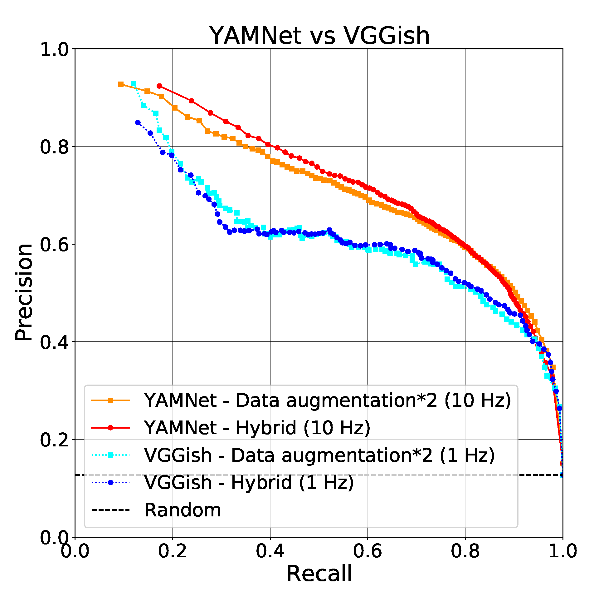
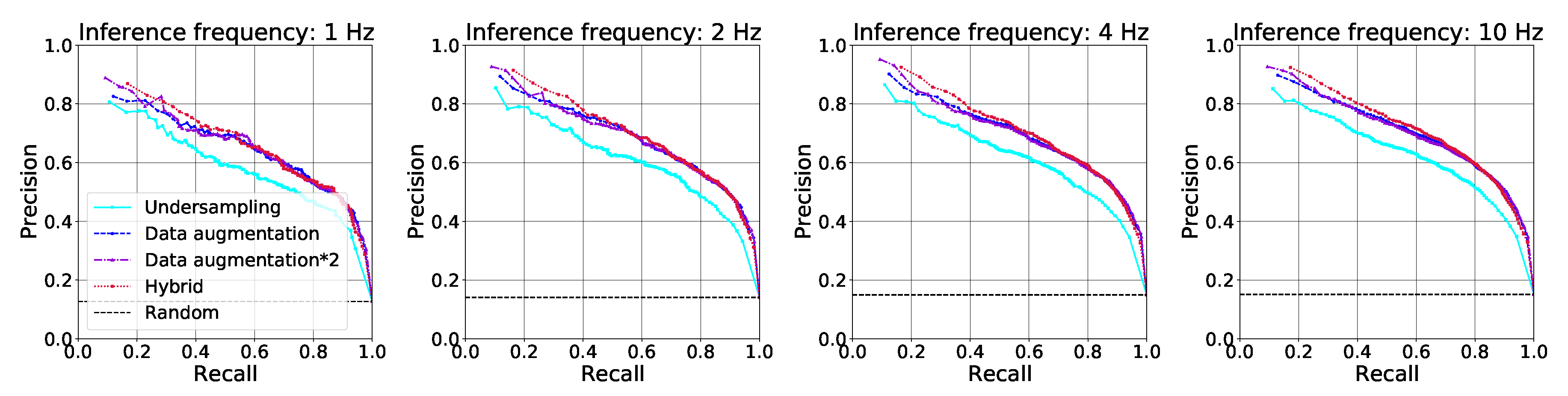
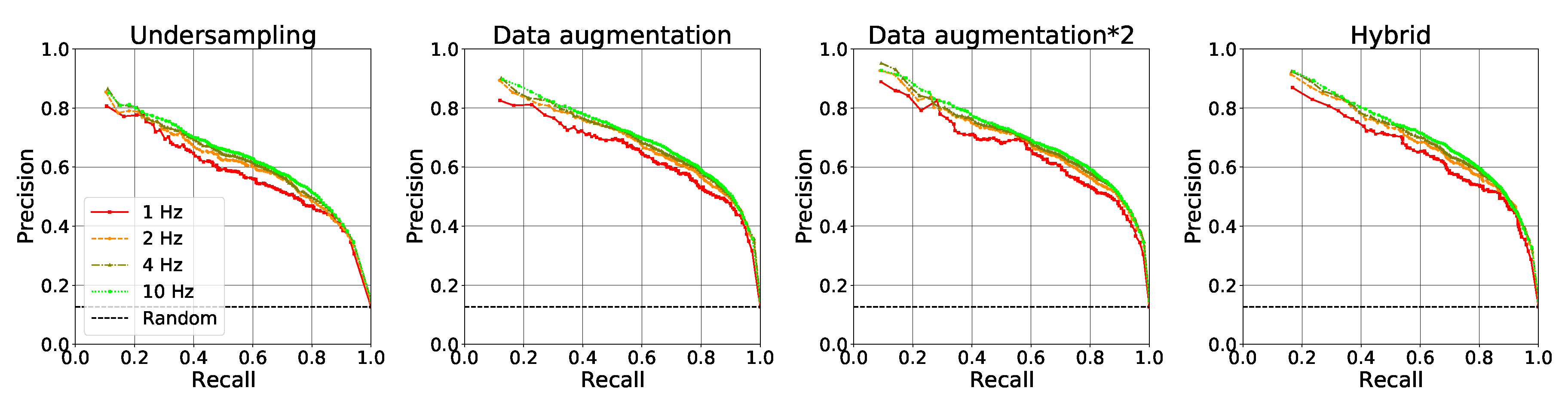
3.2. Dataset and Inference Frequency Comparison

Each model is tested for each possible combination of datasets and inference frequencies, as shown in Table 3. For each inference frequency, the best T P R and F P R values are highlighted in bold. Furthermore, for each model, the best overall T P R and F P R are highlighted in red. For both models, the ‘Data augmentation*2’ and ‘Hybrid’ datasets show the best performance in terms of F P R and T P R , respectively, across all inference frequencies. The best overall performance for YAMNet and VGGish corresponds to an inference frequency of 10 Hz and 1 Hz, respectively. However, while VGGish’s best F P R (5.03%) is 1% lower than YAMNet’s (6.11%), YAMNet’s best T P R (74.90%) is 11% higher than VGGish’s (63.91%). Furthermore, the performances of each model’s best configuration are compared using Precision–Recall curves in Figure 4. Here, YAMNet also performs better than VGGish, but this time in terms of precision.
Given YAMNet’s superior performance across all datasets and inference frequencies, a more detailed analysis is performed next. Figure 5 shows the P–R curves corresponding to each inference frequency for all datasets. The largest differences in performance are observed across different datasets. For all inference frequencies, the ‘Undersampling’ dataset shows the worst performance since it suffers from the removal of 83% of ‘not aircraft’ samples without any data augmentation benefits. The ‘Data augmentation’ and ‘Data augmentation*2’ datasets benefit from the data augmentation strategies. Their performance is very similar—as evidenced by the PR curves—which indicates that, although it is beneficial to apply data augmentation to the aircraft class, further data augmentation applied to both classes has negligible effects. The ‘Hybrid’ dataset benefited both from augmenting the minority ‘aircraft’ class, and from undersampling the majority ‘not aircraft’ class to ensure class balance. Regardless of the choice of inference frequency, and excluding the ‘Undersampling’ dataset, the results for the remaining datasets are very similar for Recall > 0.7. This suggests that, in the absence of enough data representative of the minority class, a data augmentation strategy can provide a boost in prediction performance.
Figure 6 shows the P–R curves corresponding to each dataset for all inference frequencies. As the inference frequency is increased from 1 Hz to 10 Hz, performance improves for all datasets. Although it has a lower impact on performance than the choice of the dataset, there is also a clear benefit to using higher values of inference frequency.

3.3. Computational Performance Assessment

To assess the computational performance of both models, Table 4 shows inference times—defined as the time that the computer takes to read an audio waveform, extract a feature vector, and make a prediction—for four inference frequencies. These tests are performed on an Nvidia Jetson TX2 for the task of audio-based detection alone. YAMNet’s latency is one order of magnitude smaller than that of VGGish, with an average inference time of 0.154 s for an inference frequency of 10 Hz. These differences in inference times may be explained by model parameter size (4 M for YAMNet [45] vs 133 M for VGGish [17]) and model complexity thanks to the use of depthwise-separable convolutions (which reduce the number of multiply-accumulate operations). Furthermore, RAM consumption was one order of magnitude smaller for YAMNet (35 MB) than for VGGish (360 MB) for all inference frequencies. Finally, CPU and GPU usage for both models is similar, regardless of the choice of inference frequency.
For both models, depending on the value of the inference frequency, a new inference may start before the previous one has finished, meaning that two or more inferences will be computed in parallel. In the case of VGGish, high inference frequencies result in the parallel computation of dozens of inferences.

4. Conclusions

We have developed a real-time, audio-based aircraft detection system using deep learning models fine-tuned with our ‘Small Aircraft’ dataset. We have identified YAMNet—fine-tuned using our ‘Hybrid’ dataset—with an inference frequency of 10 Hz as the optimal configuration in terms of T P R and P R E . Despite the project constraints on the available computational resources, this model is able to provide accurate detection results in real-time. This study has also highlighted how data augmentation strategies can significantly improve model performance for imbalanced audio datasets. Although the aircraft type used for testing (SOCATA TB9) was different from those used for training (Edge 540, Cessna 172E, Cessna 152, and a number of historical aircraft and aircraft engines), further testing using different aircraft types will be performed in the future to strengthen our current conclusions.

Future Work

On the one hand, given the limited sample size of the ‘aircraft’ class, one immediate direction for future work is increasing the size of the ‘Small Aircraft’ dataset during additional flight campaigns using different aircraft types. On the other hand, optimizing YAMNet’s implementation to reduce feature extraction and inference computational cost would allow an even higher inference frequency and consequently a higher detection accuracy. Investigating the potential superiority of the wavelet transform over the STFT for audio post-processing [47] could also result in detection accuracy gains. Additionally, combining multiple aircraft detection systems located within a certain distance of each other and taking advantage of the microphones’ high directionality would allow us to localize the aircraft, thus increasing the utility of the current design. After some adaptation, the detection system could be integrated within a fixed-wing UAV to reduce the effect of ground sounds, while the microphones’ high directionality could also be used to minimize the effect of rotor noise. Finally, an alternative to performing inferences on the embedded computer would be to stream the audio feed via a remote connection to a cloud server. With the advent of 5G networks, this application is likely to exploit the lower latency, higher capacity, and increased bandwidth that they provide. This remote server, not being as limited by computational resources as the embedded computer onsite, would be able to use more complex SED models in real time with even higher accuracy than YAMNet.

Author Contributions

Conceptualization: V.A., F.J.P.-G. and A.V.; data curation: J.M.-H.; formal analysis: J.M.-H. and F.G.; funding acquisition: J.J.C., A.V. and A.O.; investigation: J.M.-H., V.A. and F.G.; methodology: J.M.-H., V.A. and F.G.; project administration: F.J.P.-G. and A.V.; resources: V.A. and J.J.C.; software: J.M.-H., V.A. and F.G.; supervision: V.A., J.J.C., F.J.P.-G. and A.O.; validation: J.M.-H. and F.G.; visualization: J.M.-H. and F.G.; writing—original draft: J.M.-H.; writing—review and editing: V.A., F.G. and F.J.P.-G. All authors have read and agreed to the published version of the manuscript.

Funding

This work has been partially funded by the VIGIA (ITC-20181032) and iMOV3D (CER-20191007) Spanish R&D projects, funded by the CDTI.

Acknowledgments

The authors would like to thank Carlos Albo, José Ramón López, Daniel Lozano, and Mouhsine Kassimi from CATEC for their support in gathering the dataset and integrating the system; and Justin Salamon from NYU and Adobe Research for his advice on state-of-the-art SED models.

Conflicts of Interest

The authors declare no conflict of interest.

Abbreviations

The following abbreviations are used in this manuscript:
ADS-BAutomatic Dependent Surveillance-Broadcast
ATLASAir Traffic Laboratory for Advanced Unmanned Systems
BVLOSBeyond Visual Line of Sight
CNNConvolutional Neural Network
DCASEDetection and Classification of Acoustic Scenes and Events
FNFalse Negatives
FPFalse Positives
FPRFalse Positive Rate
P–RPrecision–Recall
PREPrecision
RNNRecurrent Neural Network
RPASRemotely Piloted Aircraft Systems
SEDSound Event Detection
STFTShort-Time Fourier Transform
TNTrue Negatives
TPTrue Positives
TPRTrue Positive Rate
VLLVery Low Level

Appendix A. Nvidia Jetson TX2 Configuration and Implementation

The audio-based detection system is implemented on a Rudi Embedded System with an Nvidia Jetson TX2 embedded computer. Firstly, the Nvidia SDK manager (https://developer.nvidia.com/nvsdk-manager) and the Linux4Tegra Board Support Package (https://connecttech.com/resource-center/l4t-board-support-packages/) are downloaded. Secondly, the instructions to install the Nvidia JetPack SDK, required for artificial intelligence applications, and the Linux4Tegra Board Support Package (https://connecttech.com/resource-center/kdb375/) are followed. The detection system uses Jetpack 4.3 with TensorFlow 1.15.0 and Keras 2.2.4 installed using virtualenv 16.7. The instructions to install TensorFlow 1.15 and all other required dependencies are provided here: https://docs.nvidia.com/deeplearning/frameworks/install-tf-jetson-platform/index.html. The technical specifications of the Rudi Embedded System are:
  • GPU: 256-core Nvidia Pascal architecture (Nvidia, Santa Clara, CA, USA)
  • CPU: Dual-Core Nvidia Denver 1.5 64-Bit and Quad-Core ARM Cortex-A57 MPCore processor (Nvidia, Santa Clara, CA, USA)
  • RAM: 8 GB 128-bit LPDDR4 58.3 GB/s
  • Storage: 32 GB eMMC 5.1
Both YAMNet and VGGish are implemented on the embedded computer using a Python3 script which loads the required libraries, the CNN feature extractor, and classifier models, handles audio acquisition and processing, performs inferences at the given inference frequency (i.e., 1 Hz, 2 HZ, 4 Hz or 10 Hz), and provides the corresponding predictions.

References

  1. SESARS. European Drones Outlook Study. 2016. Available online: https://www.sesarju.eu/sites/default/files/documents/reports/European_Drones_Outlook_Study_2016.pdf (accessed on 4 September 2020).
  2. EASA. AMC & GM to Part-UAS. 2019. Available online: https://www.easa.europa.eu/sites/default/files/dfu/AMC%20%26%20GM%20to%20Part-UAS%20%E2%80%94%20Issue%201.pdf (accessed on 7 September 2020).
  3. Alarcón, V.; García, M.; Alarcón, F.; Viguria, A.; Martínez, A.; Janisch, D.; Acevedo, J.; Maza, I.; Ollero, A. Procedures for the Integration of Drones into the Airspace Based on U-Space Services. Aerospace 2020, 7, 128. [Google Scholar] [CrossRef]
  4. Murphy, J.R.; Williams-Hayes, P.S.; Kim, S.K.; Bridges, W.; Marston, M. Flight test overview for UAS integration in the NAS project. In Proceedings of the AIAA Atmospheric Flight Mechanics Conference, San Diego, CA, USA, 4–8 January 2016; p. 1756. [Google Scholar]
  5. Kim, Y.; Jo, J.Y.; Lee, S. ADS-B vulnerabilities and a security solution with a timestamp. IEEE Aerosp. Electron. Syst. Mag. 2017, 32, 52–61. [Google Scholar] [CrossRef]
  6. Otsuyama, T.; Honda, J.; Shiomi, K.; Minorikawa, G.; Hamanaka, Y. Performance evaluation of passive secondary surveillance radar for small aircraft surveillance. In Proceedings of the 2015 European Radar Conference (EuRAD), Paris, France, 9–11 September 2015; pp. 505–508. [Google Scholar]
  7. Terneux, E.A.E. Design of an Algorithm for Aircraft Detection and Tracking with a Multi-coordinate VAUDEO System. Ph.D. Thesis, Blekinge Institute of Technology, Karlskrona, Sweden, 2014. [Google Scholar]
  8. Church, P.; Grebe, C.; Matheson, J.; Owens, B. Aerial and surface security applications using lidar. In Laser Radar Technology and Applications XXIII; Turner, M.D., Kamerman, G.W., Eds.; International Society for Optics and Photonics (SPIE): Bellingham, WA, USA, 2018; Volume 10636, pp. 27–38. [Google Scholar] [CrossRef]
  9. Petridis, S.; Geyer, C.; Singh, S. Learning to Detect Aircraft at Low Resolutions. In Computer Vision Systems; Gasteratos, A., Vincze, M., Tsotsos, J.K., Eds.; Springer: Berlin/Heidelberg, Germany, 2008; pp. 474–483. [Google Scholar]
  10. Paweł, R.; Tomasz, R.; Grzegorz, J.; Damian, K.; Piotr, S.; Andrzej, P. Simulation studies of a vision intruder detection system. Aircr. Eng. Aerosp. Technol. 2020, 92, 621–631. [Google Scholar] [CrossRef]
  11. Xia, X.; Togneri, R.; Sohel, F.; Zhao, Y.; Huang, D. A Survey: Neural Network-Based Deep Learning for Acoustic Event Detection. Circuits Syst. Signal Process. 2019, 38, 3433–3453. [Google Scholar] [CrossRef]
  12. Abeßer, J. A review of deep learning based methods for acoustic scene classification. Appl. Sci. 2020, 10, 2020. [Google Scholar] [CrossRef] [Green Version]
  13. DCASE2020 Challenge Results Published—DCASE. 2020. Available online: http://dcase.community/articles/dcase2020-challenge-results-published (accessed on 5 September 2020).
  14. Hershey, S.; Chaudhuri, S.; Ellis, D.P.W.; Gemmeke, J.F.; Jansen, A.; Moore, C.; Plakal, M.; Platt, D.; Saurous, R.A.; Seybold, B.; et al. CNN Architectures for Large-Scale Audio Classification. In Proceedings of the 2017 IEEE International Conference on Acoustics, Speech and Signal Processing (ICASSP), New Orleans, LA, USA, 5–9 March 2017; pp. 131–135. [Google Scholar]
  15. Gemmeke, J.F.; Ellis, D.P.W.; Freedman, D.; Jansen, A.; Lawrence, W.; Moore, R.C.; Plakal, M.; Ritter, M. Audio Set: An ontology and human-labeled dataset for audio events. In Proceedings of the 2017 IEEE International Conference on Acoustics, Speech and Signal Processing (ICASSP), New Orleans, LA, USA, 5–9 March 2017; pp. 776–780. [Google Scholar]
  16. Krizhevsky, A.; Sutskever, I.; Hinton, G.E. ImageNet Classification with Deep Convolutional Neural Networks. Commun. ACM 2017, 60, 84–90. [Google Scholar] [CrossRef]
  17. Simonyan, K.; Zisserman, A. Very Deep Convolutional Networks for Large-Scale Image Recognition. arXiv 2015, arXiv:1409.1556. [Google Scholar]
  18. Szegedy, C.; Vanhoucke, V.; Ioffe, S.; Shlens, J.; Wojna, Z. Rethinking the Inception Architecture for Computer Vision. In Proceedings of the 2016 IEEE Conference on Computer Vision and Pattern Recognition (CVPR), Las Vegas, NV, USA, 27–30 June 2016; pp. 2818–2826. [Google Scholar]
  19. He, K.; Zhang, X.; Ren, S.; Sun, J. Deep Residual Learning for Image Recognition. In Proceedings of the 2016 IEEE Conference on Computer Vision and Pattern Recognition (CVPR), Las Vegas, NV, USA, 27–30 June 2016; pp. 770–778. [Google Scholar]
  20. Hayashi, T.; Watanabe, S.; Toda, T.; Hori, T.; Le Roux, J.; Takeda, K. Duration-Controlled LSTM for Polyphonic Sound Event Detection. IEEE/ACM Trans. Audio Speech Lang. Process. 2017, 25, 2059–2070. [Google Scholar] [CrossRef]
  21. Adavanne, S.; Pertilä, P.; Virtanen, T. Sound event detection using spatial features and convolutional recurrent neural network. In Proceedings of the 2017 IEEE International Conference on Acoustics, Speech and Signal Processing (ICASSP), New Orleans, LA, USA, 5–9 March 2017; pp. 771–775. [Google Scholar]
  22. Miyazaki, K.; Komatsu, T.; Hayashi, T.; Watanabe, S.; Toda, T.; Takeda, K. Weakly-Supervised Sound Event Detection with Self-Attention. In Proceedings of the 2020 IEEE International Conference on Acoustics, Speech and Signal Processing (ICASSP), Barcelona, Spain, 4–8 May 2020; pp. 66–70. [Google Scholar]
  23. Mnasri, Z.; Rovetta, S.; Masulli, F. Audio surveillance of roads using deep learning and autoencoder-based sample weight initialization. In Proceedings of the 2020 IEEE 20th Mediterranean Electrotechnical Conference ( MELECON), Palermo, Italy, 16–18 June 2020; pp. 99–103. [Google Scholar]
  24. Guo, X.; Su, R.; Hu, C.; Ye, X.; Wu, H.; Nakamura, K. A single feature for human activity recognition using two-dimensional acoustic array. Appl. Phys. Lett. 2019, 114, 214101. [Google Scholar] [CrossRef] [Green Version]
  25. Suero, M.; Gassen, C.P.; Mitic, D.; Xiong, N.; Leon, M. A Deep Neural Network Model for Music Genre Recognition. In Advances in Natural Computation, Fuzzy Systems and Knowledge Discovery; Liu, Y., Wang, L., Zhao, L., Yu, Z., Eds.; Springer: Basel, Switzerland, 2020; pp. 377–384. [Google Scholar]
  26. LeNail, A. NN-SVG: Publication-Ready Neural Network Architecture Schematics. J. Open Source Softw. 2019, 4, 747. [Google Scholar] [CrossRef]
  27. Salamon, J.; Jacoby, C.; Bello, J.P. A Dataset and Taxonomy for Urban Sound Research. In Proceedings of the 22nd ACM International Conference on Multimedia, New York, NY, USA, 3 November 2014; pp. 1041–1044. [Google Scholar] [CrossRef]
  28. Mesaros, A.; Heittola, T.; Virtanen, T. A multi-device dataset for urban acoustic scene classification. arXiv 2018, arXiv:1807.09840. [Google Scholar]
  29. Cartwright, M.; Mendez, A.; Cramer, J.; Lostanlen, V.; Dove, G.; Wu, H.H.; Salamon, J.; Nov, O.; Bello, J. SONYC Urban Sound Tagging (SONYC-UST): A Multilabel Dataset from an Urban Acoustic Sensor Network. In Proceedings of the Detection and Classification of Acoustic Scenes and Events 2020 Workshop (DCASE2020), New York, NY, USA, 1 October 2019; pp. 35–39. [Google Scholar] [CrossRef] [Green Version]
  30. Turpault, N.; Serizel, R.; Parag Shah, A.; Salamon, J. Sound event detection in domestic environments with weakly labeled data and soundscape synthesis. In Proceedings of the Detection and Classification of Acoustic Scenes and Events 2019, New York, NY, USA, 25–26 October 2019. [Google Scholar] [CrossRef] [Green Version]
  31. Koizumi, Y.; Saito, S.; Uematsu, H.; Harada, N.; Imoto, K. ToyADMOS: A Dataset of Miniature-machine Operating Sounds for Anomalous Sound Detection. In Proceedings of the IEEE Workshop on Applications of Signal Processing to Audio and Acoustics (WASPAA), New Paltz, NY, USA, 20–23 October 2019; pp. 308–312. [Google Scholar]
  32. Purohit, H.; Tanabe, R.; Ichige, T.; Endo, T.; Nikaido, Y.; Suefusa, K.; Kawaguchi, Y. MIMII Dataset: Sound Dataset for Malfunctioning Industrial Machine Investigation and Inspection. In Proceedings of the Detection and Classification of Acoustic Scenes and Events 2019 Workshop (DCASE2019), New York, NY, USA, 25–26 October 2019; pp. 209–213. [Google Scholar]
  33. Chen, H.; Xie, W.; Vedaldi, A.; Zisserman, A. Vggsound: A Large-Scale Audio-Visual Dataset. In Proceedings of the 2020 IEEE International Conference on Acoustics, Speech and Signal Processing (ICASSP), Barcelona, Spain, 4–8 May 2020; pp. 721–725. [Google Scholar]
  34. Trowitzsch, I.; Taghia, J.; Kashef, Y.; Obermayer, K. The NIGENS General Sound Events Database; Technical Report; Technische Universität Berlin: Berlin, Germany, 2019. [Google Scholar]
  35. Piczak, K.J. ESC: Dataset for Environmental Sound Classification. In Proceedings of the 23rd ACM International Conference on Multimedia, New York, NY, USA, 1 October 2015; pp. 1015–1018. [Google Scholar] [CrossRef]
  36. Partners In Rhyme. Free Airplane Sound Effects. Available online: https://www.freesoundeffects.com/free-sounds/airplane-10004/ (accessed on 9 June 2020).
  37. Music Technology Research Group (MTG), UPF. Freesound. Available online: https://freesound.org/search/?q=airplane (accessed on 9 June 2020).
  38. SoundBible. Airplane Sounds. Available online: http://soundbible.com/suggest.php?q=airplane&x=0&y=0 (accessed on 9 June 2020).
  39. FADA. ATLAS—Air Traffic Laboratory for Advanced unmanned Systems. Available online: http://atlascenter.aero/en/ (accessed on 9 June 2020).
  40. Rosen, S.; Howell, P. Signals and Systems for Speech and Hearing, 2nd ed.; OCLC: 706853128; lEmerald: Bingley, UK, 2011. [Google Scholar]
  41. More, S.R. Aircraft Noise Characteristics and Metrics. Ph.D. Thesis, Purdue University, West Lafayette, IN, USA, 2011. [Google Scholar]
  42. Salamon, J.; Bello, J.P. Deep Convolutional Neural Networks and Data Augmentation for Environmental Sound Classification. IEEE Signal Process. Lett. 2017, 24, 279–283. [Google Scholar] [CrossRef]
  43. Google. YAMNet. 2019. Available online: https://github.com/tensorflow/models/tree/master/research/audioset/yamnet (accessed on 9 June 2020).
  44. Google. VGGish. 2019. Available online: https://github.com/tensorflow/models/tree/master/research/audioset/vggish (accessed on 9 June 2020).
  45. Howard, A.G.; Zhu, M.; Chen, B.; Kalenichenko, D.; Wang, W.; Weyand, T.; Andreetto, M.; Adam, H. MobileNets: Efficient Convolutional Neural Networks for Mobile Vision Applications. arXiv 2017, arXiv:cs.CV/1704.04861. [Google Scholar]
  46. Davis, J.; Goadrich, M. The relationship between Precision–Recall and ROC curves. In Proceedings of the 23rd International Conference on Machine Learning (ICML ’06), New York, NY, USA, 1 June 2006; pp. 233–240. [Google Scholar]
  47. Kiskin, I.; Zilli, D.; Li, Y.; Sinka, M.; Willis, K.; Roberts, S. Bioacoustic detection with wavelet-conditioned convolutional neural networks. Neural Comput. Appl. 2020, 32, 915–927. [Google Scholar] [CrossRef] [Green Version]
Figure 1. Images captured from the ground-based system, showing a small aircraft (SOCATA TB9) flying at a distance of two kilometers. Image resolution: 5472 × 3648 (20 MP); angle of view: 32.9 (horizontal) and 24.8 (vertical). Long-range detection poses a challenge to both image and audio-based strategies.
Electronics 09 02076 g001
Figure 2. Proposed ‘Detect and Avoid’ system which goes from capturing a sound to detecting an aircraft. CNN and classifier schematics generated using NN-SVG [26].
Electronics 09 02076 g002
Figure 3. Audio post-processing and feature extraction applied to one of the audio waveforms from the ‘Small Aircraft’ dataset.
Electronics 09 02076 g003
Figure 4. Precision–Recall curves comparing YAMNet and VGGish’s best-performing configurations.
Electronics 09 02076 g004
Figure 5. YAMNet Precision–Recall curves comparing each dataset for different inference frequencies.
Electronics 09 02076 g005
Figure 6. YAMNet Precision–Recall curves comparing each inference frequency for different datasets.
Electronics 09 02076 g006
Table 1. Sample size for the ‘aircraft’ and ‘not aircraft’ classes, defined as the number of feature vectors extracted from the audio waveforms for each dataset.
DatasetAircraft Sample SizeNot Aircraft Sample Size
Small Aircraft21,398244,750
Undersampling21,39840,247
Data augmentation215,746244,750
Data augmentation*2427,916446,765
Hybrid135,910154,759
Table 2. Range of values for different data augmentation strategies.
AugmentationTime Stretch, %Resampling, %Volume Change, %Random Noise, %
Value range75–15090–11065–120±1
Table 3. YAMNet and VGGish performance according to T P R and F P R , expressed as a percentage, for four datasets and four inference frequencies.
Inference Frequency
ModelsDatasets1 Hz2 Hz4 Hz10 Hz
TPR , % FPR , % TPR , % FPR , % TPR , % FPR , % TPR , % FPR , %
YAMNetUndersampling66.448.9266.208.6465.678.7365.838.35
Data augmentation71.267.1770.186.9869.376.8869.866.64
Data augmentation*268.056.2767.496.2567.086.3467.456.11
Hybrid74.488.6574.748.2574.548.0774.907.77
VGGishUndersampling62.766.8462.697.0061.617.3162.007.61
Data augmentation56.785.6056.265.6656.915.9557.066.20
Data augmentation*253.565.0354.045.1454.795.2654.345.73
Hybrid63.916.2463.746.3563.326.3662.816.68
Table 4. YAMNet and VGGish inference times (mean ± standard deviation) (s) for four inference frequencies.
ModelsInference Frequency
1 Hz2 Hz4 Hz10 Hz
YAMNet0.140 ± 0.0220.144 ± 0.0260.138 ± 0.0260.154 ± 0.018
VGGish1.637 ± 0.0731.632 ± 0.0521.618 ± 0.0611.637 ± 0.086
Publisher’s Note: MDPI stays neutral with regard to jurisdictional claims in published maps and institutional affiliations.

