Proposal of an Adaptive Fault Tolerance Mechanism to Tolerate Intermittent Faults in RAM

Abstract

Due to transistor shrinking, intermittent faults are a major concern in current digital systems. This work presents an adaptive fault tolerance mechanism based on error correction codes (ECC), able to modify its behavior when the error conditions change without increasing the redundancy. As a case example, we have designed a mechanism that can detect intermittent faults and swap from an initial generic ECC to a specific ECC capable of tolerating one intermittent fault. We have inserted the mechanism in the memory system of a 32-bit RISC processor and validated it by using VHDL simulation-based fault injection. We have used two (39, 32) codes: a single error correction–double error detection (SEC–DED) and a code developed by our research group, called EPB3932, capable of correcting single errors and double and triple adjacent errors that include a bit previously tagged as error-prone. The results of injecting transient, intermittent, and combinations of intermittent and transient faults show that the proposed mechanism works properly. As an example, the percentage of failures and latent errors is 0% when injecting a triple adjacent fault after an intermittent stuck-at fault. We have synthesized the adaptive fault tolerance mechanism proposed in two types of FPGAs: non-reconfigurable and partially reconfigurable. In both cases, the overhead introduced is affordable in terms of hardware, time and power consumption.

1. Introduction

In the last years, the reduction of transistor size has increased microprocessor speed and density while decreasing their supply voltage. However, this size reduction has provoked an increment in the incidence of faults. In this way, bit error rates for transient faults, commonly caused by temporary environmental conditions, or permanent faults, whose origin are irreversible physical changes in a chip, are now much higher [1,2]. The extreme transistor size reduction has provoked, as a side effect, a dramatic diminution in the critical charge required to switch the logical state of transistors [3]. Thus, the impacts of subatomic particles (i.e., alpha particles, neutrons, etc.) in electronic devices may alter even multiple cells.

In recent times, intermittent faults have emerged as a new source of trouble in deep submicron integrated circuits that affect a wide range of industries [4]. Traditionally considered as a prelude to permanent faults, the introduction of new deep submicron technologies has originated intermittent faults that do not end up necessarily in permanent faults [5].

The main causes of intermittent faults are manufacturing defects and residues, process variations and wear-out mechanisms. These faults occur non-deterministically at the same location, and they are usually grouped in bursts. Additionally, they may be activated or deactivated by changes in temperature, voltage or frequency [6]. The processes needed to manufacture integrated circuits with increasingly smaller transistors require correspondingly greater precision. Thus, apparently, negligible process variations may cause serious future defects that can be undetected in the post-manufacturing test. These manufacturing defects may become shorts, open circuits, or capacitance or resistance variations. When these effects manifest intermittently (for instance, due to process, voltage or temperature (PVT) variations), they provoke intermittent faults.

Albeit errors induced by transient and intermittent faults manifest in a similar way, intermittent faults affect the system repeatedly during their activation. This makes them a good candidate to identify and apply a special treatment. The question that arises is how we can distinguish between transient and intermittent faults. As far as we know, the different attempts to decide between these two fault types have been theoretical/simulated [7,8,9]; or by using a complete and dedicated system to identify intermittent faults [10].

For these types of faults, it is advisable to use fast detection/recovery techniques, mainly hardware- or hybrid-implemented. The high speed of silicon logic makes hardware implementations well suited for detection and correction of high rate errors. In addition, combined hardware error detection and recovery with software implemented failure prediction and resource reconfiguration may improve dependability significantly [6,11]. Due to their high speed and low cost, error control codes (also known in the literature as “error correction codes” and “error-correcting codes”, ECC) present a very successful detection/recovery behavior. Established for more than half a century, ECCs have been extensively employed in computer systems to protect information against errors [12].

Single errors (i.e., those errors that affect only one bit in a binary word) are the most common ones. Thus, single error correction (SEC) and single error correction-double error detection (SEC-DED) codes are frequently included in memory designs to enhance their reliability. For instance, Hamming codes [13] allow single error correction with minimum redundancy and simple and fast encoding and decoding operations. Hamming codes, like most ECCs, are designed assuming that all bits in a word have the same probability of becoming erroneous.

However, intermittent faults pose a new problem. When a bit is affected by an intermittent fault, this bit will present a different bit error rate (BER) than the rest of the bits in a word. That is, some bits may be affected by more errors than other bits in the same word (i.e., variable bit error rate, VBER). Hence, when a bit in a memory word is affected by an intermittent fault, eventual transient faults affecting the same word may become multiple faults, not corrected by static ECCs (such as Hamming SEC or SEC-DED, BCH—Bose–Chaudhuri–Hocquenghem, or OLS—orthogonal Latin square-codes).

Hence, deep submicron circuits are exposed to two sources of faults that coexist and even can overlap: environmental conditions (causing transient faults) and internal conditions (provoking intermittent faults). This exacerbates the probability of multiple faults occurring in space and time. Thus, in our opinion, it would be interesting to adapt error correction capabilities to work with different bit error rates. A possibility is the use of special ECCs able to cope with changing bit error rates. For instance, flexible unequal error control (FUEC) codes [14] can divide codewords into any required number of areas, establishing for each one the adequate error detection and/or correction levels. These codes can be implemented by using simple logic operations, allowing fast encoding and decoding.

As a rule of thumb, static ECCs can cope with uniform bit error rates, but not when BER is variable. (F)UEC codes are good when the BER variation is spatial, but when the variation is temporal (as in the case of intermittent faults), ECCs themselves cannot cope with an unpredictable variation in the BER. That is why the adaption becomes necessary: by changing the ECC used (choosing from a set of static or unequal ECCs), the system can afford better the changes in the fault hypothesis.

In this work, we present an adaptive fault-tolerance (AFT) mechanism [15], which is able to detect and identify intermittent errors in the RAM, especially sensitive to faults [6,16,17,18,19,20,21,22,23,24]. After identifying an intermittent error, the AFT mechanism changes its behavior in order to adapt to the presence of this type of errors. The AFT mechanism was designed at a low level (i.e., hardware-implemented), based in ECCs, speeding up in this way its operation. Then, it was inserted in the memory system of Plasma, a 32-bit reduced instruction set computing (RISC) microprocessor without interlocked pipeline stages (MIPS), with a four-stage pipeline [25].

To assess the behavior of the AFT mechanism in the presence of faults, we have used VHDL simulation-based fault injection, a particular simulation-based fault injection (SBFI) technique based on the use of VHDL (very high speed integrated circuit hardware description language) as modeling language which has proven to be a good technique to study the impact of intermittent faults [11,26,27,28]. It is a useful experimental way to evaluate the dependability of a system during the design phase. An early diagnosis allows saving costs in the design process, avoiding redesigning in case of error, and thus reducing time-to-market.

The main concept underlying our proposal is its ability to reconfigure itself when error conditions get worse. FPGAs are mainly used as a support to partial reconfiguration. Moreover, given that FPGAs are being used to synthesize microprocessors for some time [29,30], we have used an FPGA-synthesizable core as the basis for our design, such as Plasma.

Currently, FPGAs can reach relatively high performance and even are being used to accelerate neural networks [31]. Moreover, now that the microprocessor-developing companies have associated with FPGA developers [32,33], probably the concept of reconfiguration may join to microprocessors. If this may happen one day, a variety of possibilities in the field of fault-tolerance will open.

The paper is organized as follows: In Section 2, we show some previous work on fault-tolerance mechanisms (FTM) in memories. Section 3 depicts the adaptive fault tolerance (AFT) mechanism proposed to detect and tolerate intermittent faults. In Section 4, we describe the fault injection experiments carried out to assess the AFT mechanism, analyze its behavior in the presence of faults, and discuss the overhead induced when synthesized in an FPGA. Finally, Section 5 provides some conclusions and outlines future work.

2. Related Work

Manufacturers and scientists have been trying to minimize the effects of faults for decades. Their work is devoted mainly to the reduction of the soft error rate (SER), that is to say, to diminish the impact of faults caused by radiation. However, modern advances in manufacturing processes also augment the error rate due to intermittent faults.

Memories have been signaled as the source of a high percentage of failures in computer systems. In this section, we will summarize some works related to the improvement of fault tolerance in memories. However, to the best of our knowledge, little work is devoted to two areas:

• The detection and correction of intermittent faults, which are an important issue in systems where reparation is difficult (like space ships) or in critical systems (like car or airplane driving systems).
• The ability to modify online the operation of the system when error conditions vary.

Whilst the concept of adaptive fault tolerance (AFT) is well known since the end of the 1980s [34], it has been mainly devoted to large-scale distributed computer systems, and only software techniques have been used [34,35,36,37,38,39]. In Reference [40], a pre-scheduled reconfigurable fault tolerance mechanism is presented. The idea is to tailor the fault tolerance technique used to the foreseen radiation levels in a space ship orbit. The system is synthesized in a reconfigurable FPGA, so it is possible to change the coverage level by partially reconfiguring the FPGA. Although this system is adaptable and hardware-implemented, the reconfiguration is not triggered by changes detected by the system; instead, they are pre-scheduled. In Reference [41], Shin et al. propose an adaptive ECC with three correction capabilities (1-, 2- and 4-errors) that adapts depending on the error frequency, which is analyzed in the control unit. Similarly, Silva et al. present in [42] CLC-adaptive, a column line code-based ECC able to activate CLC-Extended decoder depending on the result of initial CLC-standard decoding.

One of the major concerns related to sensitivity to faults in memories is fault multiplicity. Indeed, the reduction of the feature size has provoked that particle impacts can cause multiple faults [3,43] (i.e., spatial multiplicity). On the other hand, temporal fault multiplicity [43] can be provoked when uncorrected errors accumulate in the same memory location, or register caused by faults occurred at different time instants and due to various origins. In both cases, the result is the same: traditional ECCs used in memories (mainly SRAMs in caches and DRAMs) cannot correct multiple faults. This increases the number of caches (at all levels) misses, slowing the read operation, and eventually, increasing the number of failures due to faults in memory. Some techniques existing to improve fault tolerance in memories are:

• Write-back [44]. If faults are corrected in a read operation, the correct data are written back at the end of the read operation. In this way, faults due to environmental causes can be corrected.
• Scrubbing. This consists of reading, correcting and rewriting back the information stored in the memory [45]. It should not be confused with the memory refresh performed in DRAM memories. A refresh consists of merely reading to a buffer the physical information stored and writing it back. Instead, in a scrubbing, the information is read, and the ECC used is applied to correct (if possible) existing errors; then, the corrected data together with the recalculated ECC are written back.

There are two formats: patrol scrubbing and demand scrubbing [46]. Patrol scrubbing is performed periodically and automatically and may be started by either the memory controller (when the memory is idle) or the CPU (when the system is idle). Demand scrubbing is performed in every memory read, not to be confused with the aforementioned write-back; in that case, the rewrite operation is carried out only when an error has been corrected.

Reference [41] studies whether scrubbing is really necessary for cache memories. Considering the cache size and the FIT (failure in time), the authors calculate the DUE (detected unrecoverable errors) rate, and they assert that scrubbing is necessary only in very large (from hundreds of megabytes) caches.

Regarding adaptive mechanisms that can modify the memory operation, we have found in the literature some proposals. In Reference [47], Chishti et al. propose a technique that allows the operating system to adaptively change the cache size and ECC capability to adjust to cache operating conditions, particularly when switching between normal and low voltage operation modes. In [48], Datta & Touba propose a similar approach to phase change memories (PCM). Again, the ECC and the memory size are adapted over time as the number of failed cells in the phase change memory accumulates. The operating system monitors the number of errors corrected on each memory line, and when the number of errors on a line begins to exceed the strength of the currently used ECC, the ECC strength is adaptively increased while the memory capacity reduces. In Reference [49], Kim et al. propose an adaptive memory controller that can opt between multiple scheduling schemes to enhance memory performance. These adaptive systems are software implemented, and they are not applied to tolerate intermittent faults. Particularly, the proposal in [49] is devoted exclusively to enhance performance. More recently, there are efforts to develop adaptive hardware schemes to enhance the reliability and/or yield of NAND flash memories ([50,51], out of the scope of this work) and PCM. Reference [52] proposes to use a separate DRAM to store check bits for faulty rows in a PCM array. When a non-faulty row is read, data are extracted directly from the PCM array. When a faulty row is read, a long codeword (including check bits) is read from the PCM and the DRAM, and data are decoded from it. In Reference [53], Chen et al. propose an SEU monitor (basically, an error counter) to be integrated into an SRAM with EDAC (error detection and correction) and scrubbing.

To end up, there exist in the literature a few works related to detect intermittent faults. Apart from the works mentioned in the Introduction (theoretical/simulated [7,8,9], or using an identification system [10]), there are others implemented at high abstraction levels. For instance, Wang et al. [54] propose a software intermittent fault detector based on signature analysis, and Ebrahimi and Kerkhoff propose a system to detect intermittent resistive faults at the board level [55,56].

3. Design of an Adaptive Fault Tolerance Mechanism

We can see in the literature a lack of research and development related to low-level hardware-implemented AFT mechanisms devoted to detect and tolerate intermittent faults. With this work, we intend to fill this gap and propose a fault-tolerance mechanism able to detect intermittent faults in the RAM and adapt its operation to increase the protection of the faulty bit without increasing the redundancy.

In addition, we have inserted this AFT mechanism into the VHDL model of the Plasma microprocessor [24]. Plasma has a 32-bit MIPS architecture with a four-stage pipeline. The VHDL model of Plasma is described at register transfer (RT) and Logic abstraction levels.

3.1. Methodology

First, we will describe the general methodology followed to make the microprocessor adaptive. Then, we will focus on the particular case study implemented, where the system is able to detect intermittent faults and adapt its behavior.

Making the microprocessor adaptive affects three elements of the Plasma model (see Figure 1):

• The size of internal memory was augmented in order to store data bits together with their corresponding code bits. Considering that the ECCs used have redundancy of r bits, the 512 × 32 original RAM was changed to a 512 × (32 + r) RAM.
• Consequently, the data bus length also grows in r bits.
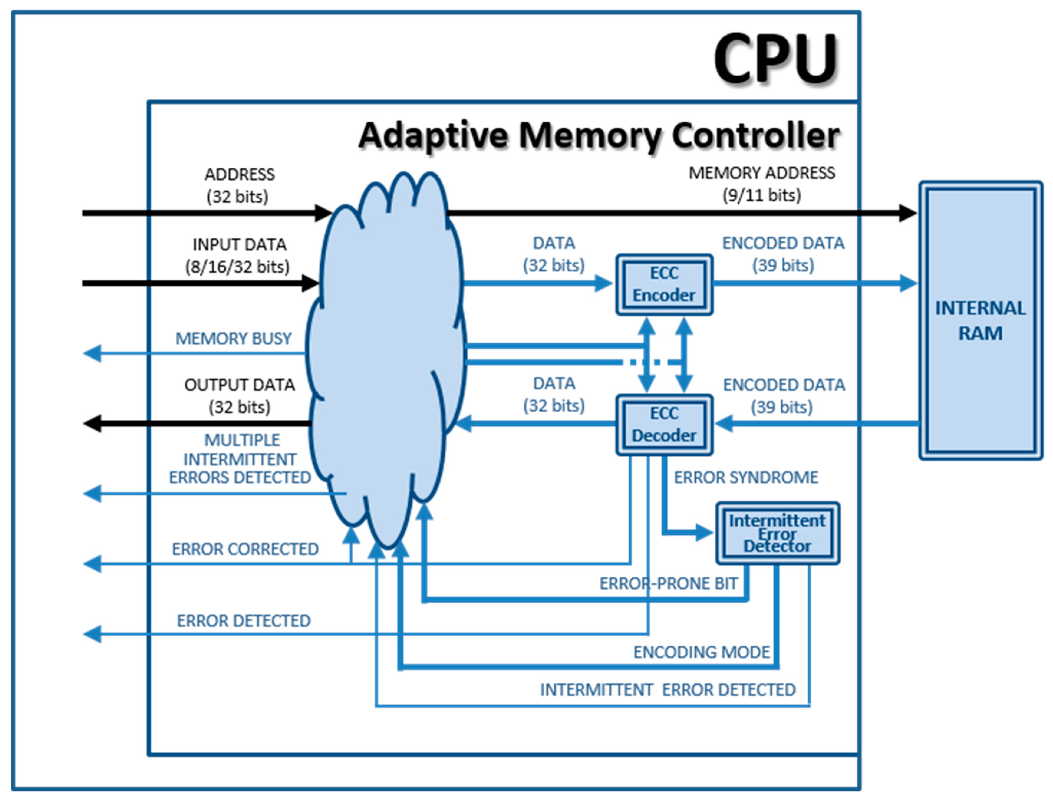
• The “Memory Controller” module that we have renamed as “Adaptive Memory Controller” in the adaptive version. The mission of this component in the original (non-fault-tolerant) Plasma core is to manage the access to the internal RAM from the CPU. In the adaptive version, the memory controller will also:
  • support the ECCs implemented,
  • detect changes in the error condition, and
  • manage the adaption process.

The first step to make the memory controller fault-tolerant is to provide some FTM. As based on ECCs, it would require:

• Adding r code bits to data from the CPU (to be written in memory), or encoding operation;
• Removing the r code bits from data read from memory (to be sent to the CPU). In addition, in case of existing errors, data should be corrected (if errors are covered by the active ECC). This operation is called decoding.

Remark that the encoding and decoding circuits are intimately related to the particular ECC used.

Hence, far, this scheme matches any fault-tolerant ECC-based mechanisms. In our case, we intend to design a component able to detect changes in the error conditions and, if possible, to replace encoding and decoding circuits with others corresponding to a new ECC able to tolerate the new error condition. We call this operation monitoring. An important premise of our proposal is the fact that all the ECCs used must have the same redundancy. The reason is to keep the same memory (and data bus) size in every system evolution, thus reducing the complexity gap between different operating versions of the system.

The block diagram of the adaptive version of the Plasma microprocessor (Plasma_ADAPTIVE core) can be seen in Figure 1; Figure 2 shows the block diagram of the “Adaptive Memory Controller” module. The colored elements are those added or modified with respect to the original model.

For a later understanding of how the AFT proposed works, we will now describe how memory read and write operations work in the Plasma model (where “ECC Encoder” and “ECC Decoder” modules in Figure 2 are not present). The RAM is asynchronous, and the memory controller is implemented as a state machine. Both operations are started by the memory controller and the last clock cycle. Regarding reading operation (see Figure 3a), during the read cycle: (1) The memory controller sets the memory address and the read signal (with a delay t_d). (2) The memory returns the contents of the indicated address (after t_access). Then, the data can be buffered and delivered to the control unit (3), respecting both the buffer setup time (t_su) and the memory read hold time (t_rh). In the write cycle (see Figure 3b): (1) The memory controller sets the data to be written, the memory address and the write signal (after a delay t_d). (2) The data are written in the indicated address (respecting the memory write setup and hold times, t_wsu and t_wh). Obviously, the minimum system clock period must be equal to max(T_r(cyc), T_w(cyc)).

“ECC Encoder” and “ECC Decoder” modules work like this:

• During a write operation (see Figure 3d), the “ECC Encoder” calculates a code from the input data (adding a delay t_enc), and both are stored together in the memory.
• In a read operation, the encoded data are obtained from the RAM. The “ECC Decoder” uses the data part of the memory word read to calculate the corresponding code, and then, the calculated code and the stored code are compared, generating a syndrome vector. This syndrome vector will mark if an erroneous bit(s) is(are) present or not and if error(s) can be corrected or detected. If there are no errors (see Figure 3c, where t_dec represents all the delay introduced by the decoder: syndrome generation and data correction), read data can be buffered and delivered to the control unit. If error(s) can be corrected, the output data will be corrected by the decoder and then buffered and delivered; also, the corrected data are re-encoded and written-back in the memory (see Figure 3e). In this case, the memory controller stops the processor during the write-back cycle by setting the “MEMORY BUSY” signal (see Figure 2).

Comparing the timing diagrams of Plasma and Plasma_ADAPTIVE cores in Figure 3, we can assert how the ECC affects the operating frequency: the delays introduced by the ECC encoder and decoder may enlarge the minimum clock period, hence decreasing the maximum clock frequency.

To implement the adaptive version of the memory controller, some considerations must be made first:

• Both “ECC Encoder” and “ECC Decoder” modules must implement the encoders and decoders of at least two different ECCs.
  When errors are detected, but cannot be corrected, the “ECC Decoder” module issues the “Error Detected” signal to warn the control unit. This signal is set under distinct circumstances, depending on the error correction and detection capabilities of the ECC used.
• The system starts operating with the simplest ECC (let us name it ECC1).
• An error monitor module monitors the occurrence of errors. As the memory degrades, either because the number of upsets increments or because errors in the same location repeatedly appear (manifesting the appearance of an intermittent fault), the error monitor module should be able to detect the new error condition, and it may be necessary to change from current ECC (let us name ECCi) to another ECC (ECCj, j ≠ i) able to cope with the new error condition.
• If there are no more ECCs available after detecting a new error condition, the “Adaptive Memory Controller” should issue some warning or error signal to the control unit (e.g., see “MULTIPLE INTERMITTENT ERRORS DETECTED” in Figure 2).
• Error conditions are not supposed to improve, but only to get worse. That is, if fault multiplicity increases, it will not decrease back again. Similarly, once a bit has been labeled as “error-prone” (i.e., an intermittent fault has been detected in that bit), it will never be unlabeled. If anything, a second (or more) bit could also be labeled as “error-prone”.

To monitor the occurrence of errors, the error monitor module contains a number of counters. From the error syndrome vector, the “Syndrome Decoder” indicates which bit(s) has/have failed, incrementing the corresponding counter(s). To count error events, we have based on the α-count single threshold-based fault identification mechanism proposed by Bondavalli et al. in [8]:

$${\alpha }^{\left(L\right)}= \{\begin{array}{cc}{\alpha }^{\left(L-1\right)}+1& if J^{\left(L\right)}=1\\ {\alpha }^{\left(L-1\right)}-dec& if \begin{array}{c}{J}^{\left(L\right)}=0 AND {\alpha }^{\left(L-1\right)}-dec>0,\\ 0\le dec\end{array} \\ 0& if J^{\left(L\right)}=0 AND {\alpha }^{\left(L-1\right)}-dec\le 0\end{array}$$

(1)

where α is the value of the counter, and J is a system binary signal that represents that an error has been detected.

When a counter surpasses a predetermined threshold (α_TH, that can be configured in the model), it overflows. This means that a change in the error conditions has been detected. Then, the AFT mechanism (i.e., the adaptive memory controller) should be reconfigured. This is carried out in four steps (see Figure 1 and Figure 2):

• The microprocessor is stopped (by setting the aforementioned “MEMORY BUSY” signal), and the “ECC Encoder” module is changed to the corresponding to the new ECC to be used;
• The whole RAM is scrubbed by reading all memory addresses sequentially using the old “ECC Decoder” to get the data and re-encoding them with the new “ECC Encoder”. This operation is similar to the faulty read shown in Figure 3e, and hence it takes two clock cycles per memory address;
• The “ECC Decoder” is changed to the corresponding to the new ECC to be used;
• The microprocessor is resumed (unsetting “MEMORY BUSY”), continuing its operation from the same point.

3.2. Case Example: Intermittent Fault Detection

As a case example, we have designed an adaptive memory controller able to detect intermittent faults. For the sake of simplicity, we have assumed that only single faults can occur, at least before the system wearout.

Given the fault hypothesis, the system will use two ECCs generated by using the FUEC methodology [14]: a typical Hsiao-based (39, 32) SEC-DED code [57] and an EPB3932 [58]. The EPB3932 code is also a (39, 32) code, but with some special features: it has asymmetric error control (it is an Unequal Error Control, UEC, code) so that it can tolerate intermittent faults in one bit, marked as an error-prone bit (EPB). It was generated to be able to correct single errors, double (both adjacent and random) errors that contain the EPB, and triple-adjacent errors containing the EPB; it also can detect double-adjacent errors (not containing the EPB).

SEC-DED is a common ECC used in memory systems. EPB3932 is a code with the same redundancy (7 bits) as SEC-DED, but it has unbalanced correction capabilities, as it overprotects the corresponding EPB. It is important to remark that, as the EPB3932 applies special error control to the EPB, unlike the SEC-DED, this code is not uniform for all 39 bits in the codeword. Instead, there is a different EPB3932 code for each bit, and each of them has its associated “ECC Encoder” and “ECC Decoder” modules.

In this case example, the only monitoring mission of the error monitor module is to detect the occurrence of an intermittent error in a memory bit. For this reason, we have named this module an “Intermittent Error Detector” in Figure 2.

Figure 4 shows the block diagram of the “Intermittent Error Detector” module. There, notice the 39 error counters, one per codeword bit. Regarding Equation (1), in the counters, J (generated by the “Syndrome Decoder”) represents now that an error has been corrected in the corresponding bit, and dec = 1. If dec = 0, the counter would be simpler, but it may detect false positives. By setting dec = 1, only errors corrected consecutively in the same bit will be considered as originated by intermittent faults.

From our fault hypothesis, we assume that the occurrence of consecutive errors (as many as the α_TH threshold) in the same bit is very unlikely unless they are due to an intermittent error. Hence, we have considered that consecutive errors corrected in the same bit must belong to the same memory word. For this reason, the number of error counters in the “Intermittent Error Detector” coincides with the codeword length (i.e., 39).

The operation of the “Adaptive Memory Controller” module is as follows: When the system starts, the SEC-DED code is selected as encoding mode. When a read error is corrected in bit i, the “Intermittent Error Detector” module increases the “BITi counter” (and decrements the other counters). If the count surpasses the predetermined threshold (α_TH), then an alleged intermittent fault is detected, and the bit i is marked as EPB. In that case, the “Intermittent Error Detector” module activates the “INTERMITTENT ERROR DETECTED” signal and sets “ERROR PRONE BIT” and “ENCODING MODE” values to force the reconfiguration of the adaptive memory controller. Then, the system should switch the “ECC Encoder”, the “ECC Decoder”, and the “Syndrome Decoder” circuits to those of the EPB3932 code for the bit i.

To implement the Plasma_ADAPTIVE model, we have modified the VHDL description of the Plasma model [24], implementing all the modules described. We have tried two different synthesis strategies.

First, we have synthesized the system in a non-reconfigurable device (see description in Section 4.5). We will refer to this version as “static”. Figure 5 shows a detail of the “Adaptive Memory Controller” for this synthesis approach. Note that the actual number of different encoders and decoders (i.e., m in the figure) is 40, one for the SEC-DED code and 39 for all the EPB3932 codes.

This synthesis approach has the advantage of reducing the reconfiguration latency of the system because the change of the “ECC Encoder” module takes just one clock cycle, and the change of the “ECC Decoder” and the “Syndrome Decoder” takes another clock cycle. Indeed, as the multiplexers and demultiplexers in Figure 4 are controlled by signals generated by the logic circuitry in the “Adaptive Memory Controller” from “ERROR PRONE BIT” and “ENCODING MODE” signals (see Figure 2), to activate a different ECC, it is only necessary to change those signals, which is made in one single clock cycle.

Thus, the reconfiguration latency required for this approach is two clock cycles plus the scrubbing latency, which depends on the memory size only. However, it has a notable drawback: all possible versions of the reconfigurable modules must be present in the device. This provokes high area overhead and (apparently) greater power consumption (see Section 4.5).

Second, we have synthesized the system in a reconfigurable FPGA (see description in Section 4.5). In this case, we have adapted the Plasma_ADAPTIVE model to allow this feature, adding an external module to manage the FPGA reconfiguration. We will refer to this version as “dynamic”.

Figure 6 shows the block diagram for this synthesis approach. The “Reconfiguration Manager” module in the figure is external to the microprocessor (although synthesized in the same FPGA), and the “Configuration ROM” module is a permanent memory (a flash card, for example) external to the FPGA that stores the bitstreams of all the modules that should be reconfigured in case of swap (i.e., “ECC Encoder”, “ECC Decoder” and “Syndrome Decoder”). The mission of the “Reconfiguration Manager” is to read a bitstream file from the “Configuration ROM” and reconfigure a module in the FPGA, as indicated by the “Adaptive Memory Controller”.

This approach has the important advantage of reducing the complexity of the system considerably in terms of hardware usage, as only one version of the reconfigurable circuits is physically present in the device. This greatly diminishes the area overhead. Its main drawback is the time consumed to reconfigure the modules, increasing the reconfiguration latency.

In Section 4.5, we will discuss the overhead introduced by each of these synthesis approaches.

3.3. Other Cases

In this paper, we present a particular implementation example of the Adaptive Fault Tolerance Mechanism proposed. However, for other fault hypotheses, any other codes (or even more than two) could be used. It would be sufficient to change their corresponding “ECC Encoder” and “ECC Decoder” modules, as well as the “Syndrome Decoder” module in the “Error Monitor” module (instead of “Intermittent Error Detector”) in Figure 2.

In addition, it would be possible to reconfigure the adaptive memory controller due to other changes in the error conditions, such as detecting an iteration in the occurrence of a particular fault multiplicity or others. That would depend on the fault hypothesis of the system.

Anyway, it would be necessary to find evolutions of the initial ECC able to overprotect any error-suspicious bits (or change the error coverage), but without increasing the redundancy. This is one of the main premises of our proposal.

4. Assessment of the Adaptive Fault Tolerance Mechanism

To assess the performance of the AFT mechanism proposed, we have scheduled a number of injection campaigns that we describe in the following. It is interesting to mention that, for simulation purposes, we have set the threshold to detect intermittent errors (i.e., α_TH) to 5. This is a tradeoff value, big enough to prevent from detecting false positives and small enough to permit detecting faults in the short duration of the workload (2686 clock cycles). In addition, we have set the clock period to 100 ns (nanoseconds), the default value in the original Plasma model.

Prior to validating the operation on the proposed model, we have analyzed the simulation of the Plasma model, annotating every memory access (including the address and the access time). From this analysis, we have extracted some important features of the workload, such as the number of times that each memory address is accessed, the average access time (i.e., the average separation between accesses), and the time of the last access.

4.1. Fault Injection Parameters

The injection parameters configured in the injection campaigns can be classified into seven groups:

• Fault injection technique. We have used simulator commands, a VHDL simulation-based fault injection technique [59]. This technique allows changing, at simulation time, the value or the timing of the signals and variables of a VHDL model.
• Injection targets. Faults have been injected in the internal RAM of the Plasma microprocessor, running the Bubblesort sorting algorithm. This algorithm sorts 10 integer values. The size of the algorithm is 72 memory words (out of 512 of the whole memory) for the code segment, plus 30 words for the data segment. Therefore, only 102 memory addresses out of 512 (a 20%) are actually accessed by the workload.
  Bubblesort algorithm is an adequate workload to check the performance of the AFT mechanism proposed because it accesses multiple times memory addresses (belonging to both code and data segments). This allows to inject faults in the same memory location at different operation times (simulating intermittent faults) and analyze if they are corrected or detected by the AFT mechanism. On the other hand, the duration of this workload makes the duration of the injection campaign to be reasonable.
  We have considered running other workloads, but we have discarded them because either they do not access the data segment enough times to allow detecting intermittent faults in it, or their simulation times are unfeasible.
• Number of faults injected. Each injection experiment consists of a number of model simulations where a set of faults is injected in each simulation.
  We have studied a suitable number of injections per experiment. In tuning experiments, we have injected experiments with 1000 and 10,000 injections. The results differ by less than 1%. Hence, we have opted for injecting 1000 faults per experiment.
• Fault models. As commented in the Introduction, besides transient faults, intermittent faults are a major challenge in modern computer design, as detecting and tolerating them is not an easy task. Thus, we have injected these two types of faults.
  Consequent to the injection target (i.e., RAM cells), the fault models injected are bit-flip for transient faults and intermittent stuck-at and intermittent bit-flip for intermittent faults [22]. For short, we will refer to them as BF, ISA and IBF hereinafter.
  Regarding intermittent fault models, ISA and IBF differ in their behavior after fault deactivation; in ISA faults, the effect of fault disappears, and the target recovers the previous value; in IBF faults, however, the erroneous value persists in time until it is overwritten.
• Fault timing. As the bit-flip just consists of inverting the logic value of the affected cell, the duration of transient faults does not make sense.
  The timing of intermittent faults depends on some variable aspects like manufacturing process, environment, wearout process, etc. In this way, three burst parameters must be taken into account to model intermittent faults [60]:
  • Burst length (L_Burst). It represents the number of times that the fault is activated in the burst.
  • Activity time (t_A). It indicates the duration of each fault activation. In IBF faults, the activity time does not make sense. In ISA faults, we have defined three ranges: [0.1T, T], [T, 10T] and [10T, 100T], where T is the clock cycle.
  • Inactivity time (t_I). It is the separation between two consecutive activations. Due to their different behavior, we have defined different settings for this parameter. In IBF faults, we have the average access time (i.e., the average separation between accesses, obtained from the workload analysis, see Section 4), which is different for each memory address. Instead, in ISA faults, we have defined three ranges: [0.1T, T], [T, 10T] and [10T, 100T].
  The reason to use the average access time in IBF faults is to reduce the probability that two (or more) consecutive activations may occur between two consecutive accesses. If an even number of fault activations occurred prior to memory access, they would cancel in pairs, reducing the effect of the intermittent fault.
• Fault multiplicity. Transient faults may affect multiple locations due to technology scaling [5]. These multiple locations can be adjacent (i.e., neighbor cells in registers and memory, neighbor wires in a bus, etc.) or non-adjacent (i.e., random). Thus, we have injected both single and multiple faults in both random and adjacent bits (in the same memory word). In addition, multiple transient faults can occur when a single transient fault coincides with a previously uncorrected error [41], no matter what its origin is. We have also injected this type of multiple faults, particularly an intermittent fault followed by single and multiple transient faults.
• Measurements. The data measured are:
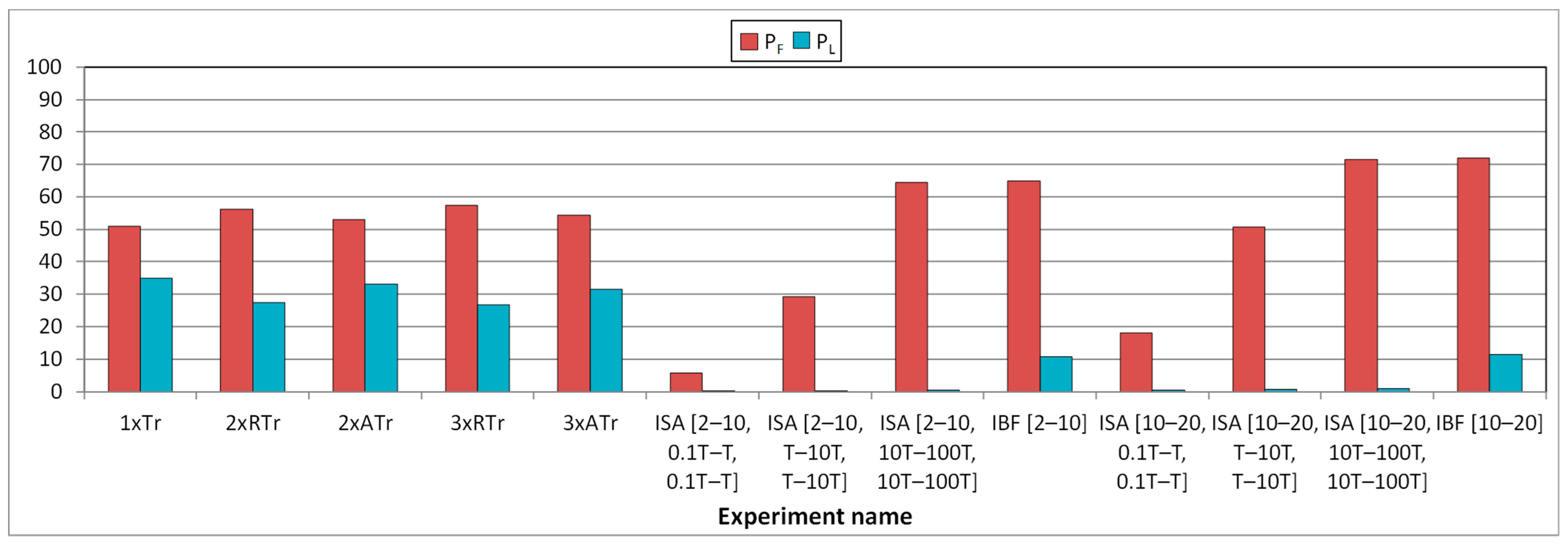
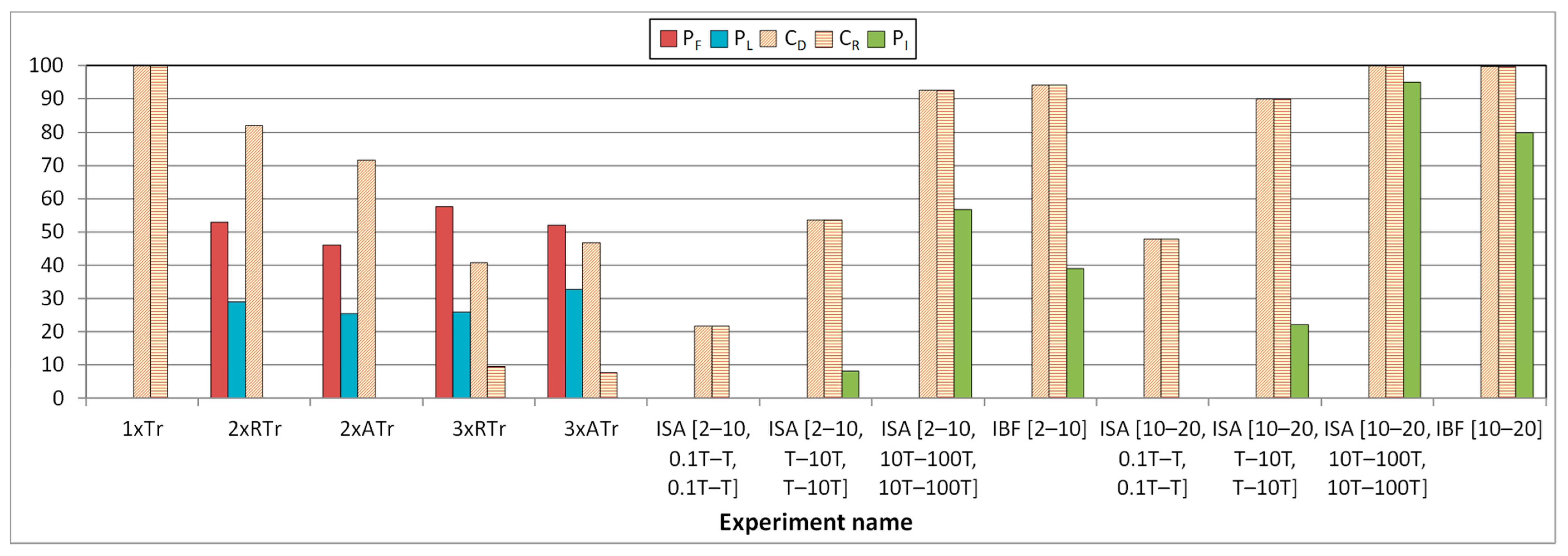
  • The percentage of failures, P_F:

    $${\mathrm{P}}_{\mathrm{F}}=\frac{{\mathrm{N}}_{\mathrm{F}}}{{\mathrm{N}}_{\mathrm{inj}}}\times 100,$$

    (2)

    where N_F is the number of failures, and N_inj is the number of injections (i.e., simulations).
  • The percentage of latent errors, P_L:

    $${\mathrm{P}}_{\mathrm{L}}=\frac{{\mathrm{N}}_{\mathrm{L}}}{{\mathrm{N}}_{\mathrm{inj}}}\times 100,$$

    (3)

    where N_L is the number of latent errors.
  • The detection coverage, C_D:

    $${\mathrm{C}}_{\mathrm{D}}=\frac{{\mathrm{N}}_{\mathrm{D}}}{{\mathrm{N}}_{\mathrm{inj}}}\times 100,$$

    (4)

    where N_D is the number of errors detected.
  • The recovery coverage, C_R:

    $${\mathrm{C}}_{\mathrm{R}}=\frac{{\mathrm{N}}_{\mathrm{R}}}{{\mathrm{N}}_{\mathrm{inj}}}\times 100,$$

    (5)

    where N_R is the number of errors corrected.
  • The percentage of intermittent errors detected, P_I:

    $${\mathrm{P}}_{\mathrm{I}}=\frac{{\mathrm{N}}_{\mathrm{I}}}{{\mathrm{N}}_{\mathrm{inj}}}\times 100,$$

    (6)

    where N_I is the number of intermittent errors detected.

To distinguish between failures and latent errors, we have classified the memory addresses into two categories. First, we have denoted the memory addresses where the workload results are stored (being part of the data segment) as system outputs so that a value different from the simulation without faults will be considered as a failure. Second, we have denoted the rest of the memory addresses (including the code segment, the remaining of the data segment, and other unused addresses) as internal elements; in these addresses, a value different from the simulation without faults will be considered as a latent error.

4.2. Injection Experiments

We have scheduled a number of injection experiments on the models based on different fault scenarios:

• Single transient faults;
• Double and triple random (in the same memory word) transient faults;
• Double and triple adjacent (in the same memory word) transient faults;
• Single intermittent faults;
• Single intermittent faults combined with single and multiple transient faults in the same memory word. These experiments simulate the occurrence of a transient fault in the same memory word after an intermittent error has been detected, the system has been reconfigured with a new ECC, and the memory has been scrubbed. The objective of these experiments is to check the behavior of the system after the reconfiguration.

The multiple transient faults include double and triple random, double and triple adjacent, double pseudorandom, double pseudo-adjacent and triple pseudo-adjacent. The “pseudo-” refers to the fact that one of the faulty bits must be the bit labeled as EPB during the detection of the intermittent fault. Hence, if a bit is marked as EPB upon the intermittent fault injection, this bit will be mandatorily injected in the following pseudo-multiple transient fault injection after the ECC is swapped.

In the experiments, the values of the parameters defined with ranges have been calculated using a uniform distribution function.

4.3. Injection Campaign

In this section, we present the results of injecting faults under some controlled injection conditions:

• The set of injection targets are limited in each experiment to those memory addresses that are accessed by the workload, and only if they are accessed (at least) as many times as the maximum number of fault activations of the fault to be injected. That is to say, a memory address that is accessed 15 times during the workload execution will be selected as the target when injecting intermittent faults with a burst length in the range [2, 10], but not in the range [10, 20].
• Faults are injected in each target in a time window where the addresses are accessed. We know these time windows from the workload analysis (see Section 4).

With these conditions, we prevent injecting faults in memory addresses that will not be accessed after the injection. In this way, we reduce the probability of the fault to become a latent error, increasing the likelihood of becoming an error.

From the tuning experiments, we can assert that a latent error may be due to two main reasons:

• The injected fault modified a memory address but did not cause any failure.
• The fault was injected after the last access to that address, or the address was never accessed.

Next, we will show a subset of the outcomes obtained from the injection campaign.

4.4. Outcomes

In Figure 7, Figure 8 and Figure 9 we show the results of injecting some types of faults into Plasma and Plasma_ADAPTIVE cores under controlled conditions, as described above.

Figure 7 shows the influence of faults in the Plasma core. It includes (in X-axis) the following experiments:

• Single transient faults (labeled as 1xTr);
• Double random transient faults (2xRTr);
• Double adjacent transient faults (2xATr);
• Triple random transient faults (3xRTr);
• Triple adjacent transient faults (3xATr);
• Single intermittent faults. From all the experiments carried out (varying the fault model, L_burst, t_A and t_I), we have selected a subset:

  o

  Intermittent stuck-at (ISA) fault model, with L_burst in the range [2, 10], t_A in the range [0.1T, T], and t_I in the range [0.1T, T], where T is the clock cycle of the system (labeled as ISA [2–10, 0.1T–T, 0.1T–T] in the graph).

  o

  ISA fault model, with L_burst in the range [2, 10], t_A in the range [T, 10T], and t_I in the range [T, 10T] (ISA [2–10, T–10T, T–10T]).

  o

  ISA fault model, with L_burst in the range [2, 10], t_A in the range [10T, 100T], and t_I in the range [10T, 100T] (ISA [2–10, 10T–100T, 10T–100T]).

  o

  Intermittent bit-flip (IBF) fault model, with L_burst in the range [2, 10] (IBF [2–10]).

  o

  ISA fault model, with L_burst in the range [10, 20], t_A in the range [0.1T, T], and t_I in the range [0.1T, T] (ISA [10–20, 0.1T–T, 0.1T–T]).

  o

  ISA fault model, with L_burst in the range [10, 20], t_A in the range [T, 10T], and t_I in the range [T, 10T] (ISA [10–20, T–10T, T–10T]).

  o

  ISA fault model, with L_burst in the range [10, 20], t_A in the range [10T, 100T], and t_I in the range [10T, 100T] (ISA [10–20, 10T–100T, 10T–100T]).

  o

  Intermittent bit-flip (IBF) fault model, with L_burst in the range [10, 20] (IBF [2–10]).

For each experiment, two columns are presented, representing (in the Y-axis) the percentage of failures (P_F) and the percentage of latent errors (P_L) (see Section 4.1).

From the figure, we can confirm that transient faults provoke high percentages of failures (P_F) plus latent errors (P_L) (about 85%). The remaining 15% of faults injected are masked by the system operation, usually due to a later write operation. As this model does not use any fault tolerance mechanism, fault multiplicity does not have any influence, and all transient faults have similar incidence.

However, the effect of intermittent faults depends very much on the fault model, the fault timing, and the burst length. Indeed, only ISA faults with burst lengths in the range [10, 20] and t_A in the range [T, 10T], ISA faults with t_A in the range [10T, 100T], and IBF faults, provoke percentages of failures similar to or higher than transient faults. Nevertheless, only IBF faults cause latent errors, though much less than transient faults. The motive of these different figures caused by ISA and IBF faults lies in their different behavior: in IBF faults, the erroneous value persists after fault deactivation, whereas in ISA faults, it does not.

On the other hand, these lower values of P_F (in certain cases) and P_L caused by intermittent faults are due to several factors:

• When injecting ISA faults with t_A in the range [0.1T, T], it is very unlikely to access a memory address affected by a fault. Moreover, this probability reduces for smaller numbers of fault activations. This implies that most fault activations do not affect the system. However, this probability grows as t_A does, causing more failures than transient faults.
• Something different occurs to IBF faults: if a fault activation does not affect the system, the next activation will cancel the effect of the previous one, thus reducing its damage.

In Figure 8, we can see the effects of the same fault types in the behavior of the Plasma_ADAPTIVE core. In this figure, besides P_F and P_L, in the Y-axis, we have also calculated the detection and recovery coverages (C_D and C_R), as well as the percentage of intermittent errors detected (P_I). These parameters do not make sense in the Plasma core, and for this reason, they did not appear in Figure 7.

From the figure, we can observe that all single (transient or intermittent) faults provoke 0% of both failures and latent errors. Regarding coverages, 100% of single transient faults are corrected, whereas, in the case of intermittent faults, these coverages depend on the fault model, the fault timing, and the burst length. Similar to Plasma core, the recovery coverages get to 100% only in intermittent faults with burst length in the range [10, 20] (and particularly IBF faults and ISA faults with t_A and t_I in the range [10T, 100T]).

Regarding the percentage of intermittent faults detected, they take values near to 100% only in ISA faults with L_Burst in the range [10, 20] and t_A in the range [10T, 100T] (in the figure, only the experiment with t_I in the range [10T, 100T] is shown). The reason for this behavior lies in the nature of intermittent faults described earlier: not all intermittent errors can be detected because some fault activations are masked, either because the memory address affected is not accessed while erroneous (if caused by an ISA fault) or because they cancel in pairs (if caused by an IBF fault).

Concerning multiple transient faults, we can observe that the recovery coverage is 0% in all cases, while 100% of failures plus latent errors are detected in case of double faults. This is an expected result, as the Plasma_ADAPTIVE core starts operating with the SEC-DED code, which only can detect double faults.

In this figure, we can also observe a natural masking effect in multiple transient faults, but in this case, it is between 15% and 30%.

Figure 9 depicts the behavior of Plasma_ADAPTIVE core in the presence of combined faults. In this case, we have combined an ISA fault model, with L_burst in the range [10, 20], t_A in the range [10T, 100T], and t_I in the range [10T, 100T] with the following transient (BF) faults occurred after the ECC swap:

• Single faults (labeled in the X-axis as 1xTr ×);
• Double random faults (2xRTr);
• Double pseudorandom faults (2xPsRTr);
• Double adjacent faults (2xATr);
• Double pseudo-adjacent faults (2xPsATr);
• Triple random faults (3xRTr);
• Triple adjacent faults (3xATr);
• Triple pseudo-adjacent faults (3xPsATr).

As explained in Section 4.2, the “pseudo-” experiments mean that the bit detected as EPB is mandatorily affected in the transient injection performed after the system swap.

Like in Figure 8, five columns are presented per experiment: the percentage of failures (P_F), the percentage of latent errors (P_L), the detection and recovery coverages (C_D and C_R), and the percentage of intermittent errors detected (P_I). Note that the percentage of intermittent errors detected is about 95% in all cases. This is because it only depends on the initial intermittent fault injection (corresponding to ISA [10–20, 10T–100T, 10T–100T] experiment in Figure 7), and thus the behavior is always the same.

The rest of the measurements depend on both the intermittent fault and the subsequent transient fault. We can observe that in all cases covered by the EPB3932 code (that is, single -1× Tr label-, double random including the EPB -2× PsRTr-, double adjacent including the EPB -2× PsATr-, and triple adjacent including the EPB -3× PsATr-), both correction and detection coverages are 100%. In addition, 100% of double adjacent faults are detected. Hence, we can confirm that it meets its specifications (see Section 3).

When coverages are smaller (that is, when the transient fault is not tolerated by the EPB3932 code), we can see percentages of failures of between 5% and 10%. Note the special case of the 2× ATr column, where the detection coverage is 100%. Remember that the EPB3932 code can detect all double adjacent faults (except those that include the EPB, which are corrected).

Thus, we can conclude that our proposal works properly, and the AFT mechanism is able to detect and correct the errors specified in each ECC; and when the number of errors corrected in a bit reaches the configured threshold (α_TH), it considers that the bit is suffering an intermittent error, and reconfigures itself to adapt to the new fault hypothesis. In this way, the adaptive system tolerates intermittent and combined (intermittent+transient) faults, as the significant reduction of failures and latent errors demonstrates.

4.5. Analysis of System Overhead

In this section, we analyze the overhead from two points of view. First, we compare the temporal overhead of the two versions of Plasma_ADAPTIVE core (i.e., the static version, synthesized in a non-reconfigurable FPGA and the dynamic version, synthesized in a reconfigurable FPGA) by comparing their latencies. Moreover second, we have synthesized three cores: Plasma, Plasma_SECDED and both versions of the Plasma_ADAPTIVE in the two FPGAs, and compared their hardware overhead. We have included the Plasma_SECDED core (which implements an SEC-DED code and performs write-back on correction) for comparison purposes only, as it is an intermediate design between the non-fault-tolerant Plasma and the adaptive Plasma_ADAPTIVE proposed.

Regarding the temporal overhead, we can classify system latencies in two groups: (i) detection and recovery latencies of transient errors, and (ii) reconfiguration latencies after intermittent error detection.

Detection and recovery latencies do not depend actually on the AFT mechanism, but on the fault conditions (that is, on the fault model and timing) and on the average time that the target is accessed by the workload. Thus, it is very difficult to get a representative trend.

Reconfiguration latencies, instead, do depend strongly on the actions taken by the AFT mechanism once an intermittent fault is detected. In this way, the reconfiguration latency of the static version of Plasma_ADAPTIVE core is:

$${\mathrm{t}}_{\mathrm{r}\mathrm{e}\mathrm{c}\mathrm{o}\mathrm{n}\mathrm{f}\mathrm{i}\mathrm{g}\mathrm{u}\mathrm{r}\mathrm{a}\mathrm{t}\mathrm{i}\mathrm{o}\mathrm{n}}=\left(2\mathrm{W}+2\right)\times \mathrm{T},$$

(7)

where W is the size of the memory in (39-bit) words, and T is the clock cycle. This value comes from the sum of the duration of the following actions:

• Switching the “ECC Encoder” (one clock cycle, as explained in Section 3.2), which corresponds to step 1 of the reconfiguration algorithm, is described in Section 3.1;
• Scrubbing the memory (two clock cycles per memory address; in total, 2 × W clock cycles), which corresponds to step 2;
• Switching the “ECC Decoder” and the “Error Manager” (one clock cycle) of step 3.

Hence, switching the ECC encoder and decoder is relatively fast and independent of the memory size (W). The highest temporal cost is due to the scrubbing, which is directly proportional to W. For the case study presented, where T = 100 ns and W = 512, we have t_{reconfiguration}(static) = 102.4υs (microseconds).

In the dynamic version of Plasma_ADAPTIVE core, the reconfiguration latency is given by:

$${\mathrm{t}}_{\mathrm{r}\mathrm{e}\mathrm{c}\mathrm{o}\mathrm{n}\mathrm{f}\mathrm{i}\mathrm{g}\mathrm{u}\mathrm{r}\mathrm{a}\mathrm{t}\mathrm{i}\mathrm{o}\mathrm{n}}=\left(2\mathrm{W}+2\right)\times \mathrm{T}+{\mathrm{t}}_{\mathrm{e}}+{\mathrm{t}}_{\mathrm{d}}+{\mathrm{t}}_{\mathrm{m}},$$

(8)

where t_e, t_d and t_m are the reconfiguration times of “ECC Encoder”, “ECC Decoder” and “Error Manager” modules in the FPGA.

The reconfiguration time of a module depends on the FPGA technology (i.e., the timing of the Processor configuration access port (PCAP) used to reconfigure the FPGA), the read timing from the “Configuration ROM”, and the size of the bitstream file to be written. We can estimate with the following expression:

$${\mathrm{t}}_{\mathrm{r}\mathrm{e}\mathrm{c}\mathrm{o}\mathrm{n}\mathrm{f}\_\mathrm{m}\mathrm{o}\mathrm{d}\mathrm{u}\mathrm{l}\mathrm{e}}=\frac{\mathrm{M}}{\mathrm{R}\mathrm{O}{\mathrm{M}}_{\mathrm{r}\mathrm{e}\mathrm{a}\mathrm{d}\_\mathrm{r}\mathrm{a}\mathrm{t}\mathrm{e}}}+{\mathrm{t}}_{\mathrm{P}\mathrm{C}\mathrm{A}\mathrm{P}\_\mathrm{i}\mathrm{n}\mathrm{i}\mathrm{t}}+\frac{\mathrm{M}}{\mathrm{P}\mathrm{C}\mathrm{A}{\mathrm{P}}_{\mathrm{t}\mathrm{r}\mathrm{a}\mathrm{n}\mathrm{s}\mathrm{f}\mathrm{e}\mathrm{r}\_\mathrm{r}\mathrm{a}\mathrm{t}\mathrm{e}}},$$

(9)

where M is the size of the bitstream file (in megabytes), t_{PCAP_init} is a fixed initialization delay of the port (in seconds), and ROM_{read_rate} and PCAP_{read_rate} are, respectively, the read from the ROM and write to the PCAP rates (in megabytes per second).

Now, let us study the hardware overhead. All the three cores (i.e., Plasma, Plasma_SECDED and Plasma_ADAPTIVE) have been synthesized in two different types of device: in a non-reconfigurable FPGA and in a reconfigurable FPGA. We will calculate in each case the hardware required, the maximum operating frequency reached, and the power consumption.

As a reconfigurable FPGA, we have used a Zynq-7 ZC702 (Xilinx, San Jose, CA, USA) evaluation board, which incorporates a Xilinx XC7Z020-1CLG484C SoC [61]. This FPGA includes an integrated ARM^® Cortex^®-A9 MPCore™, which is able to perform the logic reprogramming. As a non-reconfigurable FPGA, the same device can be used, just ignoring the ARM microprocessor.

Please note that we have used this FPGA only to test the performance of the design proposed. Finding the best device for a particular application of the AFT mechanism is out of the scope of this paper.

Table 1. Synthesis of Plasma cores in the non-reconfigurable FPGA.

	Full Model							Mem_Ctrl		RAM
	Hardware		Max. Speed		Power Consumption (W)			Hardware		Hardware
	LUTs	FFs	fmax (MHz)	Tmin (ns)	Dynamic	Static	Total	LUTs	FFs	LUTs	FFs
Plasma	1834	448	100	10	0.009	0106	0.115	189	103	281	0
Plasma_SECDED	2040	380	83.33	12	0.005	0103	0.108	344	35	341	0
Plasma_ADAPTIVE (static)	10,652	586	58.82	17	0.006	0103	0.109	8985	241	341	0

and

Table 2. Synthesis of Plasma cores in the reconfigurable FPGA.

	Full Model							Mem_Ctrl		RAM
	Hardware		Max. Speed		Power Consumption (W)			Hardware		Hardware
	LUTs	FFs	fmax (MHz)	Tmin (ns)	Dynamic	Static	Total	LUTs	FFs	LUTs	FFs
Plasma	1852	478	100	10	1.600	0.145	1.745	189	103	281	0
Plasma_SECDED	2054	410	100	10	1.573	0.140	1.713	344	35	341	0
Plasma_ADAPTIVE (static)	10,180	616	66.67	15	1.573	0.141	1.714	8985	241	341	0
Plasma_ADAPTIVE (dynamic)	2770	617	83.33	12	1.574	0.141	1.715	-	-	341	0

show, respectively, the comparison of the syntheses of the three models in the two devices (i.e., the XC7Z020 FPGA configured as non-reconfigurable in Table 1 and as reconfigurable in Table 2). Obviously, even though only synthetizing the dynamic version of Plasma_ADAPTIVE core (see Section 3.1) makes sense, we have synthesized all the designs in the reconfigurable FPGA for comparison purposes only.

In tables, we distinguish the data synthesis of the full model and of the memory controller and RAM components. From the synthesis report, we can obtain the hardware resources required by the whole system as by selected components. However, the maximum speed is reached, and the power consumption is only available for the full system.

At a glance, we can observe in tables that the operation of the ARM processor in the reconfigurable FPGA introduces an important increment in the power consumption (over 1.5 watts). In addition, we can note the increment in the hardware required to implement the RAM from the original Plasma core to the other fault-tolerant cores (see “RAM” column in tables).

Regarding the cores, we can note that the overhead introduced by the ECC encoding and decoding circuits in the Plasma_SECDED core is not very important in terms of hardware or power consumption. On the contrary, the maximum operating frequency gets reduced (although only in the non-reconfigurable FPGA). Note that the “Mem_ctrl” column shows the hardware required by the memory controller component, including all the ECC-associated circuitry, the write-back management and the “Error manager” component (in Plasma_ADAPTIVE cores). Remark that, in fact, the fault-tolerant and all adaptive versions reduce the power consumption in both FPGAs.

On the other hand, the static version of Plasma_ADAPTIVE core introduces a very high increment in the hardware required (about 5 × LUTs and 1.5 × FFs compared to Plasma_SECDED core), as well as a strong reduction of the maximum operating frequency. As explained in Section 3.1, in this version, all the encoding and decoding circuits are physically implemented in the memory controller (see Figure 5). Nevertheless, the increment of the power consumption is very subtle (only one milliwatt). This trend occurs in the two FPGAs.

Finally, the dynamic version of the Plasma_ADAPTIVE core (see Figure 6) introduces much less hardware overhead (about 1.35 × LUTs and 1.5 × FFs compared to the Plasma_SECDED core) than the static version. In addition, the power overhead is small (a few milliwatts), and the maximum operating frequency does not reduce dramatically. In this row, we can miss the presence of information related to the “Mem_ctrl” component. It is due to the fact that this information is not available in the synthesis report because this module uses internally “Reconfiguration blocks” (those related to the reconfigurable modules: “ECC Encoder”, “ECC Decoder” and “Error Manager”, all included in the “Adaptive Memory Controller” component). For this reason, the synthesis report cannot include specific information on this component.

Regarding the reconfiguration latency of this version, assuming the same values of T and W used previously, and applying in Equation (9) the values for the XC7Z020 FPGA (t_{PCAP_init} = 0.0005 s, PCAP_{read_rate} = 120 MBytes/s), the timing of an SD card used as “Configuration ROM” (ROM_{read_rate} = 19.63 MBytes/s), and given that the size of all bitstream files is 172 KBytes, we get an overall reconfiguration time t_{reconfiguration}(dynamic) = 31.472 ms (milliseconds). Obviously, this value is no good for a hard real-time system, but searching for the more suitable FPGA for such a purpose is out of the scope of this paper.

Anyway, we consider that the overhead introduced by the adaptive fault-tolerant mechanism proposed is affordable. Even the non-reconfigurable approach could be considered if the speed is not a limit. On the other hand, the outcomes obtained are referred to only one FPGA. Probably, other devices could allow getting much better performance in the operating frequency.

4.6. Comparison with Other Proposals

Table 3. Comparison of the adaptive fault-tolerance (AFT) mechanism proposed with other previous works.

Work	Description	Memory Type	Management Implementation	Trigger	Alternative ECCs	Same Redundancy?	Physical Reconfiguration?
[41]	Adaptive ECC for cache	SRAM	Hardware	Voltage scaling	1-, 2-, 4-bit BCH	No	No
[42]	CLC with two decoding modes	Undefined	Hardware	Decoding error	CLC-S, CLC-E	Yes	No
[47]	Adaptive error correction scheme for cache	SRAM	Software	Voltage variation	SEC-DED, OLSC (varying data/code ratio)	No	Yes
[48]	Adaptive error correction scheme for PCM	PCM	Software	Number of failed cells	OLSC (varying data/code ratio)	No	Yes
[50]	Adaptive ECC for NAND flash	NAND-flash	Hardware	Bit error rate	Hamming, 2-, 4-bit BCH	No	No
Static	Static version of Plasma_ADAPTIVE	RAM	Hardware	Intermittent error	SEC-DED, EPB3932	Yes	No
Dynamic	Dynamic version of Plasma_ADAPTIVE	RAM	Hardware	Intermittent error	SEC-DED, EPB3932	Yes	Yes

shows a comparison of the two versions of our proposal with some of the previous works included in Section 2 applied to memories. In the table, besides the reference and a short description of the work, we have included aspects such as:

• The type of memory to which is applied.
• How is the adaption management implemented (hardware vs. software)?
• The adaption trigger.
• The list of alternative ECCs.
• Do the alternative ECCs have the same redundancy?
• Does the system physically reconfigure? That is to say, is the system reprogrammed/reconfigured, or are all the ECCs physically implemented in the system as spares?

In the table, we can see that most proposals use ECCs with different redundancy. From these, in the ones where no physical reconfiguration is performed ([41,42,50] and the static version of our proposal), the encoding and decoding circuitry of all ECCs is physically implemented, increasing the hardware overhead.

If we analyze the other proposal that keeps the redundancy [42], we realize that actually, only one code is implemented in the alternatives. The only difference between the alternatives is the decoding mode, being possible to opt between a simple and fast (although with fewer correction capability) mode and a higher correction capability mode (but more complex and slow).

Analyzing the ECCs used, we utilize in our proposals two simple ECCs, while in most proposals in the table, other more complex ECCs (BCH [42,50], OLSC [47,48] or CLC [42]) are applied. The reason is mainly the fault hypothesis assumed. In our proposal, we assume that only single transient faults may occur until a single intermittent fault appears.

Thus, we have selected two ECCS able to cope with these two fault hypotheses: the SEC-DED when only single transient faults occur, and the EPB3932 when an intermittent fault is detected. However, as mentioned in Section 3.3, this is only a case example, and other ECCs (either well-known or UEC evolved from traditional) could be used in the system. It just depends on the fault hypothesis. For instance, if the initial fault hypothesis is that double transient faults can occur before an intermittent fault appears, then:

• A 2-bit BCH could be used as the initial ECC.
• It should swap to another (UEC) ECC able to support at least one intermittent error plus multiple (adjacent or random) additional errors.

Compared with the proposals where physical reconfiguration is applied [47,48], only our dynamic proposal is controlled by hardware, whereas in the others, reconfiguration is carried out by the operating system.

Last but not least, the only proposals that trigger the system adaption by the detection of an intermittent error are our proposals. Others adapt to voltage scaling [41,47], to the overall number of failed cells (counted by the OS) [48], or to a calculated bit error rate stored in an internal table called “reliability map” [50]; finally, in [42] when the CLC-S decoding detects that the number of errors exceeds its error correction capabilities, it launches the second decoding in CLC-E mode.

Thus, as we have mentioned throughout the paper, this is, to our knowledge, the first work where a low-level hardware-implemented AFT mechanism is proposed to adapt to intermittent faults with no redundancy increment.

5. Conclusion and Future Work

We have developed an adaptive fault-tolerance (AFT) mechanism based on ECC codes to tolerate intermittent faults in RAM. The AFT mechanism is able to detect variations in the error condition and then change its internal configuration to adapt to a new fault hypothesis.

We have implemented a first version that employs two (39, 32) codes, an SEC-DED and an EPB3932 (able to correct all single errors, as well as double and triple adjacent errors that contain a bit which is suspect to have a higher probability of being erroneous because it has already been erroneous for a number of times).

When an “error monitor” detects that a particular bit is repeatedly erroneous, it is marked as “error-prone” (i.e., suspect to be suffering an intermittent fault) and switches to the EPB3932 code, thus covering future errors in that bit, as well as other errors.

We have designed this AFT mechanism in VHDL and integrated it into the memory controller of a 32-bit RISC microprocessor. We have stressed the system injecting single/multiple, random/adjacent, transient/intermittent, and combinations of intermittent and transient faults. From the injection experiments, we can see that the proposed AFT mechanism can detect transient faults, correct them and, in case an intermittent fault is detected, it is able to change the ECC to adapt to the new fault hypothesis.

We also analyzed the overhead introduced by the AFT mechanism proposed. From the analysis, we can assert that the overhead introduced, if synthesized in a reconfigurable FPGA, is affordable in terms of hardware and temporal overhead and power consumption. If synthesized in a non-reconfigurable FPGA, though, the proposed model introduces a hardware overhead that could be affordable.

For future work, we intend to implement both versions of the AFT mechanism in FPGA in order to inject faults to calculate their real coverages and latencies. In addition, we are developing other design alternatives studying new ECCs to be incorporated in the AFT mechanism. Another future work line is to design adaptive fault-tolerance mechanisms for other CPU elements, like the register bank.

References

1. International Technology Roadmap for Semiconductors (ITRS). 2013. Available online: http://www.itrs2.net/2013-itrs.html (accessed on 2 October 2020).
2. Jen, S.L.; Lu, J.C.; Wang, K. A review of reliability research on nanotechnology. IEEE Trans. Reliab. 2007, 56, 401–410. [Google Scholar] [CrossRef]
3. Ibe, E.; Taniguchi, H.; Yahagi, Y.; Shimbo, K.; Toba, T. Impact of scaling on neutron-induced soft error in SRAMs from a 250 nm to a 22 nm design rule. IEEE Trans. Electron Devices 2010, 57, 1527–1538. [Google Scholar] [CrossRef]
4. Boussif, A.; Ghazel, M.; Basilio, J.C. Intermittent fault diagnosability of discrete event systems: And overview of automaton-based approaches. Discret. Event Dyn. Syst. 2020. [Google Scholar] [CrossRef]
5. Constantinescu, C. Trends and challenges in VLSI circuit reliability. IEEE Micro 2003, 23, 14–19. [Google Scholar] [CrossRef]
6. Constantinescu, C. Impact of Intermittent Faults on Nanocomputing Devices. In Proceedings of the Workshop on Dependable and Secure Nanocomputing (WDSN 2007), Edinburgh, UK, 28 June 2007; pp. 238–241. [Google Scholar]
7. De Kleer, J. Diagnosing Multiple Persistent and Intermittent Faults. In Proceedings of the 21st International Joint Conference on Artificial Intelligence (IJCAI-09), Pasadena, CA, USA, 11–17 July 2009; pp. 733–738. [Google Scholar]
8. Bondavalli, A.; Chiaradonna, S.; Di Giandomenico, F.; Grandoni, F. Threshold-Based Mechanisms to Discriminate Transient from Intermittent Faults. IEEE Trans. Comput. 2000, 49, 230–245. [Google Scholar] [CrossRef]
9. Contant, O.; Lafortune, S.; Teneketzis, D. Diagnosis of Intermittent Faults. Discret. Event Dyn. Syst.-Theory Appl. 2004, 14, 171–202. [Google Scholar] [CrossRef] [Green Version]
10. Sorensen, B.A.; Kelly, G.; Sajecki, A.; Sorensen, P.W. An Analyzer for Detecting Intermittent Faults in Electronic Devices. In Proceedings of the 1994 IEEE Systems Readiness Technology Conference (AUTOTESTCON’94), Anaheim, CA, USA, 20–22 September 1994; pp. 417–421. [Google Scholar] [CrossRef]
11. Gracia-Moran, J.; Gil-Tomas, D.; Saiz-Adalid, L.J.; Baraza, J.C.; Gil-Vicente, P.J. Experimental validation of a fault tolerant microcomputer system against intermittent faults. In Proceedings of the 2010 IEEE/IFIP International Conference on Dependable Systems and Networks (DSN 2010), Chicago, IL, USA, 28 June–1 July 2010; pp. 413–418. [Google Scholar] [CrossRef]
12. Fujiwara, E. Code Design for Dependable Systems; John Wiley & Sons: Hoboken, NJ, USA, 2006. [Google Scholar] [CrossRef]
13. Hamming, R.W. Error detecting and error correcting codes. Bell Syst. Tech. J. 1950, 29, 147–160. [Google Scholar] [CrossRef]
14. Saiz-Adalid, L.J.; Gil-Vicente, P.J.; Ruiz, J.C.; Gil-Tomás, D.; Baraza, J.C.; Gracia-Morán, J. Flexible Unequal Error Control Codes with Selectable Error Detection and Correction Levels, Proceedings of the 2013 Computer Safety, Reliability, and Security Conference (SAFECOMP 2013), Toulouse, France, 14–27 September 2013; Bitsch, F., Guiochet, J., Kaâniche, M., Eds.; Lecture Notes in Computer Science; Springer: Berlin/Heidelberg, Germany, 2013; Volume 8153, pp. 178–189. [Google Scholar] [CrossRef]
15. Frei, R.; McWilliam, R.; Derrick, B.; Purvis, A.; Tiwari, A.; Di Marzo Serugendo, G. Self-healing and self-repairing technologies. Int. J. Adv. Manuf. Technol. 2013, 69, 1033–1061. [Google Scholar] [CrossRef] [Green Version]
16. Maiz, J.; Hareland, S.; Zhang, K.; Armstrong, P. Characterization of multi-bit soft error events in advanced SRAMs. In Proceedings of the 2003 IEEE International Electron Devices Meeting (IEDM 2003), Washington, DC, USA, 8–10 December 2003; pp. 21.4.1–21.4.4. [Google Scholar] [CrossRef]
17. Schroeder, B.; Pinheiro, E.; Weber, W.-D. DRAM errors in the wild: A large-scale field study. Commun. ACM 2011, 54, 100–107. [Google Scholar] [CrossRef]
18. McCartney, M. SRAM Reliability Improvement Using ECC and Circuit Techniques. Ph.D. Thesis, Carnegie Mellon University, Pittsburgh, PA, USA, December 2014. [Google Scholar]
19. Mofrad, A.B.; Ebrahimi, M.; Oborily, F.; Tahooriy, M.B.; Dutt, N. Protecting caches against Multi-Bit Errors using embedded erasure coding. In Proceedings of the 2015 20th IEEE European Test Symposium (ETS 2015), Cluj-Napoca, Romania, 25–29 May 2015; pp. 1–6. [Google Scholar] [CrossRef]
20. Kim, J.; Sullivan, M.; Lym, S.; Erez, M. All-inclusive ECC: Thorough end-to-end protection for reliable computer memory. In Proceedings of the 2016 ACM/IEEE 43rd Annual International Symposium on Computer Architecture (ISCA), Seoul, Korea, 18–22 June 2016; pp. 622–633. [Google Scholar] [CrossRef]
21. Hwang, A.A.; Stefanovici, I.; Schroeder, B. Cosmic rays don’t strike twice: Understanding the nature of DRAM errors and the implications for system design. ACM SIGPLAN Not. 2012, 47, 111–122. [Google Scholar] [CrossRef]
22. Gil-Tomás, D.; Gracia-Morán, J.; Baraza-Calvo, J.C.; Saiz-Adalid, L.J.; Gil-Vicente, P.J. Studying the effects of intermittent faults on a microcontroller. Microelectron. Reliab. 2012, 52, 2837–2846. [Google Scholar] [CrossRef] [Green Version]
23. Cai, Y.; Yalcin, G.; Mutlu, O.; Haratsch, E.F.; Cristal, A.; Unsal, O.S.; Mai, K. Error analysis and retention-aware error management for NAND flash memory. Intel Technol. J. 2013, 17, 140–164. [Google Scholar]
24. Siewiorek, D.P.; Swarz, R.S. Reliable Computer Systems: Design and Evaluation, 2nd ed.; Digital Press: Burlington, MA, USA, 1992. [Google Scholar]
25. Plasma CPU Model. Available online: https://opencores.org/projects/plasma (accessed on 2 October 2020).
26. Arlat, J.; Aguera, M.; Amat, L.; Crouzet, Y.; Fabre, J.C.; Laprie, J.C.; Martins, E.; Powell, D. Fault Injection for Dependability Validation: A Methodology and Some Applications. IEEE Trans. Softw. Eng. 1990, 16, 166–182. [Google Scholar] [CrossRef]
27. Gil-Tomás, D.; Gracia-Morán, J.; Baraza-Calvo, J.C.; Saiz-Adalid, L.J.; Gil-Vicente, P.J. Analyzing the Impact of Intermittent Faults on Microprocessors Applying Fault Injection. IEEE Des. Test Comput. 2012, 29, 66–73. [Google Scholar] [CrossRef]
28. Rashid, L.; Pattabiraman, K.; Gopalakrishnan, S. Modeling the Propagation of Intermittent Hardware Faults in Programs. In Proceedings of the 16th IEEE Pacific Rim International Symposium on Dependable Computing (PRDC 2010), Tokyo, Japan, 13–15 December 2010; pp. 19–26. [Google Scholar] [CrossRef] [Green Version]
29. Amiri, M.; Manzoor Siddiqui, F.; Kelly, C.; Woods, R.; Rafferty, K.; ·Bardak, B. FPGA-Based Soft-Core Processors for Image Processing Applications. J. Signal Process. Syst. 2017, 87, 139–156. [Google Scholar] [CrossRef] [Green Version]
30. Hailesellasie, M.; Rafay Hasan, S.; Ait Mohamed, O. MulMapper: Towards an Automated FPGA-Based CNN Processor Generator Based on a Dynamic Design Space Exploration. In Proceedings of the 2019 IEEE International Symposium on Circuits and Systems (ISCAS 2019), Sapporo, Japan, 26–29 May 2019; pp. 1–5. [Google Scholar] [CrossRef]
31. Mittal, S. A survey of FPGA-based accelerators for convolutional neural networks. Neural Comput. Appl. 2020, 32, 1109–1139. [Google Scholar] [CrossRef]
32. Intel Completes Acquisition of Altera. Available online: https://newsroom.intel.com/news-releases/intel-completes-acquisition-of-altera/#gs.mi6uju (accessed on 27 November 2020).
33. AMD to Acquire Xilinx, Creating the Industry’s High Performance Computing Leader. Available online: https://www.amd.com/en/press-releases/2020-10-27-amd-to-acquire-xilinx-creating-the-industry-s-high-performance-computing (accessed on 27 November 2020).
34. Kim, K.H.; Lawrence, T.F. Adaptive Fault Tolerance: Issues and Approaches. In Proceedings of the Second IEEE Workshop on Future Trends of Distributed Computing Systems (FTDCS 1990), Cairo, Egypt, 30 September–2 October 1990; pp. 38–46. [Google Scholar] [CrossRef]
35. González, O.; Shrikumar, H.; Stankovic, J.A.; Ramamritham, K. Adaptive Fault Tolerance and Graceful Degradation under Dynamic Hard Real-time Scheduling. In Proceedings of the 18th IEEE Real-Time Systems Symposium (RTSS’97), San Francisco, CA, USA, 3–5 December 1997; pp. 79–89. [Google Scholar] [CrossRef] [Green Version]
36. Marin, O.; Sens, P.; Briot, J.P.; Guessoum, Z. Towards Adaptive Fault Tolerance for Multi-Agent Systems. In Proceedings of the 4th European Seminar on Advanced Distributed Systems (ERSADS ’2001), Bertinoro, Italy, 14–18 May 2001; pp. 195–201. [Google Scholar]
37. Wells, P.M.; Chakraborty, K.; Sohi, G.S. Adapting to Intermittent Faults in Multicore Systems. ACM SIGOPS Oper. Syst. Rev. 2008, 42, 255–264. [Google Scholar] [CrossRef]
38. Nithyadharshini, P.S.; Pounambal, M.; Nagaraju, D.; Saritha, V. An adaptive fault tolerance mechanism in grid computing. ARPN J. Eng. Appl. Sci. 2018, 13, 2543–2548. [Google Scholar]
39. Tamilvizhi, T.; Parvathavarthini, B. A novel method for adaptive fault tolerance during load balancing in cloud computing. Clust. Comput. 2019, 22, 10425–10438. [Google Scholar] [CrossRef]
40. Jacobs, A.; George, A.D.; Cieslewski, G. Reconfigurable Fault-Tolerance: A Framework for Environmentally Adaptive Fault Mitigation in Space. In Proceedings of the 2009 19th International Conference on Field Programmable Logic and Applications (FPL), Prague, Czech Republic, 31 August–2 September 2009; pp. 199–204. [Google Scholar] [CrossRef]
41. Shin, D.; Park, J.; Paul, S.; Park, J.; Bhunia, S. Adaptive ECC for tailored protection of nanoscale memory. IEEE Des. Test 2017, 34, 84–93. [Google Scholar] [CrossRef]
42. Silva, F.; Muniz, A.; Silveira, J.; Marcon, C. CLC-A: An adaptive implementation of the Column Line Code (CLC) ECC. In Proceedings of the 33rd Symposium on Integrated Circuits and Systems Design (SBCCI 2020), Campinas, Brazil, 24–28 August 2020. [Google Scholar] [CrossRef]
43. Mukherjee, S.S.; Emer, J.; Fossum, T.; Reinhardt, S.K. Cache scrubbing in microprocessors: Myth or necessity? In Proceedings of the 10th IEEE Pacific Rim International Symposium on Dependable Computing (PRDC 2004), Papeete, Tahiti, French Polynesia, 3–5 March 2004; pp. 37–42. [Google Scholar] [CrossRef] [Green Version]
44. DeBrosse, J.K.; Hunter, H.C.; Kilmer, C.A.; Kim, K.-h.; Maule, W.E.; Yaari, R. Adaptive Error Correction in a Memory System. U.S. Patent US 2016/0036466 A1, 15 November 2016. [Google Scholar]
45. Saleh, A.M.; Serrano, J.J.; Patel, J.H. Reliability of Scrubbing Recovery-Techniques for Memory Systems. IEEE Trans. Reliab. 1990, 39, 114–122. [Google Scholar] [CrossRef]
46. Supermicro. X9SRA User’s Manual (Rev. 1.1). Available online: https://www.manualshelf.com/manual/supermicro/x9sra/user-s-manual-1-1.html (accessed on 3 October 2020).
47. Chishti, Z.; Alameldeen, A.R.; Wilkerson, C.; Wu, W.; Lu, S.-L. Improving cache lifetime reliability at ultra-low voltages. In Proceedings of the 42nd Annual IEEE/ACM International Symposium on Microarchitecture (MICRO-42), New York, NY, USA, 12–16 December 2009; pp. 89–99. [Google Scholar] [CrossRef] [Green Version]
48. Datta, R.; Touba, N.A. Designing a fast and adaptive error correction scheme for increasing the lifetime of phase change memories. In Proceedings of the 2011 29th IEEE VLSI Test Symposium (VTS 2011), Dana Point, CA, USA, 1–5 May 2011; pp. 134–139. [Google Scholar] [CrossRef]
49. Kim, J.-k.; Lim, J.-b.; Cho, W.-c.; Shin, K.-S.; Kim, H.; Lee, H.-J. Adaptive memory controller for high-performance multi-channel memory. J. Semicond. Technol. Sci. 2016, 16, 808–816. [Google Scholar] [CrossRef] [Green Version]
50. Yuan, L.; Liu, H.; Jia, P.; Yang, Y. Reliability-based ECC system for adaptive protection of NAND flash memories. In Proceedings of the 2015 Fifth International Conference on Communication Systems and Network Technologies (CSNT 2015), Gwalior, India, 4–6 April 2015; pp. 897–902. [Google Scholar] [CrossRef]
51. Zhou, Y.; Wu, F.; Lu, Z.; He, X.; Huang, P.; Xie, C. SCORE: A novel scheme to efficiently cache overlong ECCs in NAND flash memory. ACM Trans. Archit. Code Optim. 2018, 15, 60. [Google Scholar] [CrossRef] [Green Version]
52. Lu, S.-K.; Li, H.-P.; Miyase, K. Adaptive ECC techniques for reliability and yield enhancement of Phase Change Memory. In Proceedings of the 2018 IEEE 24th International Symposium on On-Line Testing and Robust System Design (IOLTS 2018), Platja d’Aro, Spain, 2–4 July 2018; pp. 226–227. [Google Scholar] [CrossRef]
53. Chen, J.; Andjelkovic, M.; Simevski, A.; Li, Y.; Skoncej, P.; Krstic, M. Design of SRAM-based low-cost SEU monitor for self-adaptive multiprocessing systems. In Proceedings of the 2019 22nd Euromicro Conference on Digital System Design (DSD 2019), Kallithea, Greece, 28–30 August 2019; pp. 514–521. [Google Scholar] [CrossRef]
54. Wang, X.; Jiang, L.; Chakrabarty, K. LSTM-based analysis of temporally- and spatially-correlated signatures for intermittent fault detection. In Proceedings of the 2020 IEEE 38th VLSI Test Symposium (VTS 2020), San Diego, CA, USA, 5–8 April 2020. [Google Scholar] [CrossRef]
55. Ebrahimi, H.; Kerkhoff, H.G. Intermittent resistance fault detection at board level. In Proceedings of the 2018 IEEE 21st International Symposium on Design and Diagnostics of Electronic Circuits & Systems (DDECS 2018), Budapest, Hungary, 25–27 April 2018; pp. 135–140. [Google Scholar] [CrossRef]
56. Ebrahimi, H.; Kerkhoff, H.G. A new monitor insertion algorithm for intermittent fault detection. In Proceedings of the 2020 IEEE European Test Symposium (ETS 2020), Tallinn, Estonia, 25–29 May 2020. [Google Scholar] [CrossRef]
57. Hsiao, M.Y. A class of optimal minimum odd-weigth-column SEC-DED codes. IBM J. Res. Dev. 1970, 14, 395–401. [Google Scholar] [CrossRef]
58. Gracia-Morán, J.; Saiz-Adalid, L.J.; Gil-Vicente, P.J.; Gil-Tomás, D.; Baraza-Calvo, J.C. Adaptive Mechanism to Tolerate Intermittent Faults. In Proceedings of the Fast Abstracts of the 11th European Dependable Computing Conference (EDCC 2015), Paris, France, 7–11 September 2015. [Google Scholar]
59. Benso, A.; Prinetto, P. (Eds.) Fault Injection Techniques and Tools for VLSI Reliability Evaluation; Kluwer Academic Publishers: Dordrecht, The Netherlands, 2003. [Google Scholar] [CrossRef]
60. Gracia, J.; Saiz, L.J.; Baraza, J.C.; Gil, D.; Gil, P.J. Analysis of the influence of intermittent faults in a microcontroller. In Proceedings of the 2008 IEEE Workshop on Design and Diagnostics of Electronic Circuits and Systems (DDECS 2008), Bratislava, Slovakia, 16–18 April 2008; pp. 80–85. [Google Scholar] [CrossRef]
61. Xilinx. ZC702 Evaluation Board for the Zynq-7000 XC7Z020 SoC. Available online: https://www.xilinx.com/support/documentation/boards_and_kits/zc702_zvik/ug850-zc702-eval-bd.pdf (accessed on 3 October 2020).
Figure 1. Block diagram of an adaptive version of the Plasma microprocessor (Plasma_ADAPTIVE) core.
Electronics 09 02074 g001
Figure 2. Block diagram of the “Adaptive Memory Controller” module implemented in Plasma_ADAPTIVE core.
Electronics 09 02074 g002
Figure 3. Timing diagrams of read and write operations in Plasma and Plasma_ADAPTIVE cores. (a) Read cycle in Plasma core; (b) write cycle in Plasma core; (c) fault-free read cycle in Plasma_ADAPTIVE core; (d) write cycle in Plasma_ADAPTIVE core; (e) faulty read in Plasma_ADAPTIVE core.
Electronics 09 02074 g003aElectronics 09 02074 g003b
Figure 4. Block diagram of the “Intermittent Error Detector” module in Plasma_ADAPTIVE core.
Electronics 09 02074 g004
Figure 5. “Adaptive memory controller”. Detail of “ECC Encoder” and “ECC Decoder” modules in the static version (synthesized in a non-reconfigurable FPGA). For simplicity, the other elements have been omitted.
Electronics 09 02074 g005
Figure 6. Block diagram of a dynamic version of Plasma_ADAPTIVE model (synthesized in a reconfigurable FPGA).
Electronics 09 02074 g006
Figure 7. Influence of faults in Plasma core. Transient and intermittent faults.
Electronics 09 02074 g007
Figure 8. Influence of faults in Plasma_ADAPTIVE core. Transient and intermittent faults.
Electronics 09 02074 g008
Figure 9. Influence of faults in Plasma_ADAPTIVE core. Combined (intermittent + transient) faults. Intermittent fault model: ISA with Lburst in the range [10, 20], tA in the range [10T, 100T] and tI in the range [10T, 100T].
Electronics 09 02074 g009