1. Introduction
There are numerous ways to describe music. One of them is categorization into music genres and their derivatives. Pieces that belong to a specific music genre have some features in common, which are the characteristics of the given genre [
1]. This can be the use of the instruments (rock, country, and electronic music), chord connections (heavy metal and brit-pop), or conditions that the music was recorded in (grunge, punk, and indie) [
2]. Furthermore, music genres are divided into smaller sub-groups that highlight specific features of the genre and are mixed to achieve a composition of new characteristics, distinctive for the given genres, such as symphonic metal and electronic rock.
The ID3 metadata container pre-defines a set of genres denoted by numerical codes. One may identify up to 191 music genres [
3], while the “standard” genre codes range from 1 to 79. The diversity of modern music shows that there is a place for many kinds of music, which means there are people who like to listen to them. Simultaneously, most people do not listen to all kinds of music; they have their preferences that are built on some musical characteristics. This is why social music services gather and explore information regarding an individual listener’s music preferences and try to support their habits by showing them a list of music they may want to choose from [
4,
5]. Even though music is most often categorized according to music genres, these services may also ask the user about his/her mood [
5,
6,
7]. This is especially important as some of the music networks are Facebook-, YouTube-, or other services-enabled platforms, such for example as Blue Note, Billboard, and Pitchfork [
8]. Daniel Ek, the co-founder of Spotify music streaming service, claims that the search and classification of music were beginning to diverge from the division into genres and should be tailored for a user [
9]. However, music networks do not ask about the personality type explicitly. Information gathered through social music services is built upon low-level, standardized parameters derived from audio signals [
10], and/or high-level semantic parameters describing music using its characteristics as well as metadata contained in the music file or statistics related to the person’s pattern of listening to music [
11,
12,
13]. As these services gather millions of users, thus the data obtained are analyzed using a similarity-based approach, having roots in statistics and do not involve advanced algorithms from the field of machine learning. However, this starts to change nowadays. In contrast, recent research studies mostly focus on the classification of music genres or emotions through machine learning or data mining techniques [
14,
15,
16,
17,
18].
Music services also collect interactions between the user and the song or between the users. A simple “interaction” means playing a song by the user and saving it to their list of the so-called “favorite songs”. This is a way of creating the user profile [
19,
20,
21]. The amount of information gathered in this process allows not only for a simple prediction of the user’s music taste but, in some cases, may lead to interesting conclusions associated with the user demographics [
22]. On many streaming platforms, personalized track lists (playlists) are also created. They are often combined with music recommendations, but have some important differences. Playlists usually have an organized structure, with songs arranged in the right sequence to maximize listener satisfaction. In the case of music recommendations, the order in which the music is played does not really matter [
13]. To maximize the listener’s satisfaction, the list should be sufficiently diverse. Playlists are available not only in a form adapted to the user’s personal preferences but also as lists of songs with a similar sound, mood, or theme, but not a personality trait. Therefore, collecting information on one’s personality may benefit music-oriented social networking and music recommendation service providers, as it can be utilized to improve quality of experience [
23]. There is a field of research connected to using such data in practical applications [
24,
25,
26]. The personality of users may be taken into account to tackle specific problems associated with, i.e., the recommendation of movies, music, or even places of interest to visit. Personality prediction may also be employed for other technical problems associated with social media such as the “new user problem” [
27], or taking into account the personality of social media users, which can be predicted from pictures they upload to the social media system [
26].
Works related to personality in music recommendation appeared relatively recently [
27,
28,
29,
30]. Laplante [
31] researched associations between music preferences and a wide variety of sociodemographic and individual characteristics, including personality traits, values, ethnicity, gender, social class, and political orientation in the context of music recommender systems. However, a basic assumption is that personality can be treated as “consistent behavior pattern and intrapersonal processes originating within the individual” [
28]. Several techniques were utilized, i.e., matrix factorization, personality-based active learning, baseline machine learning algorithms as well as deep learning of regression function [
25]. Some of these works already showed results that are promising in personality-based collaborative filtering [
25]. Even more interesting is how this topic is approached, i.e., either based on a questionnaire form or analyzing external data such as social services.
Studies on the relation between music preference and personality often use the big five traits to describe personality [
25,
31,
32,
33,
34,
35,
36,
37]. Others employ Myers–Briggs Type Indicator (MBTI) [
38], International Personality Item Pool (IPIP) [
39], or five-factor MUSIC model [
40,
41]. However, most of these works do not use music genre names or codes, but rather their description based on Short Test of Music Preferences (STOMP) [
31,
33,
34,
36,
42]. STOMP assesses four broad music-preference dimensions, i.e., reflective and complex, intense and rebellious, upbeat and conventional, and energetic and rhythmic, and is a revised version of the scale assessing preferences for 23 music genres. In contrast to the questionnaire-based studies, Nave et al. [
43] retrieved data from Facebook to answer the question of whether music preferences are related to personality traits.
Our work is a questionnaire-based study that aims to check whether features that objectively describe music can be utilized to identify one’s personality and if yes, it aims to discover what parameters are behind choosing music one listens to. Therefore, a music listening survey is implemented, which also contains a question about the personality type—introverted or extroverted.
The structure of the article is as follows.
Section 2 recalls information on related work in the area researched, particularly in the context of a person’s personality and music preference. The methodology of the subjective test employed for assessing the personality types of the participants, results of surveys, the proposed methods of the objective analysis of the musical pieces, as well as classifiers utilized, are provided in
Section 3. This is followed by showing the results of two parametrization approaches, i.e., MIRtoolbox-based [
44] and a variational autoencoder neural network [
45,
46] and the prediction employing support vector machine (SVM),
k-nearest neighbors (
k-NN), random forest (RF), and naïve Bayes (NB) algorithms (
Section 4). The results are analyzed by several statistical tests, i.e., Levene’s test, Kruskal–Wallis test, and Dunn’s post hoc test. Finally, a summary and conclusions are contained in
Section 5.
2. Music Genres and Personality Types
Studies of musical structure in either compositions or performances began as early as in ancient times. They sought out the characteristics and rules underlying a music form. This also plays a role in the music division of music into genres; it helps to analyze and describe music pieces. Classifying music into forms, styles, and genres, characterized by features such as tempo, origin, or time signature, became more and more complex with time [
47]. Initially, musical pieces were categorized as religious, chamber, and scenic (theatrical), then the subtypes were explored by Marc Scacchi in the 17th century [
48]. Subsequently, Athanasius Kircher proposed his method of dividing music [
49]. One of the definitions of musical style refers to the characteristic features occurring in the compositional technique that may be considered typical for the specific pieces, authors, nation-based, or period [
50]. Music styles and genre notions are often used interchangeably; however, one of the definitions of a music genre refers to an expressive style of music.
The division between extraversion and introversion was a concept popularized by Jung in 1921 [
51]. They represent the two types of the direction of the vital energy and cognitive focus of a person. Extraverts are outward-oriented in their thinking patterns and actions; their energy is directed towards people and things. Introverts are their extreme opposite; they focus more on their internal feelings and abstract concepts [
52]. Eysenck described extraverts as outgoing, invigorated, active, assertive, and eager for new experiences [
39]. Overall, they tend to be social. Simultaneously, introverts are described as inward, with energy directed towards concepts and ideas. Introverts are considered good listeners, preferring to speak face-to-face, and they gain their energy, unlike extraverts, from being alone. They are very in tune with their inner world.
Research by Westminster University reported by Australian Popular Science and published by the Journal of Psychology of Aesthetics, Creativity and the Arts, shows that there may be a relation between the personality and the music we prefer [
53]. The results found that some features of heavy metal make it enjoyable for people with low self-esteem. Simultaneously, a study conducted by the Heriot–Watt University of Edinburgh showed that fans of classical and metal music are mostly introverts [
54,
55]. The same study by Edinburgh’s researchers conveyed that some common characteristics describe different music recipients. Fans of country music turned out to be outgoing, punks were aggressive, and people listening to indie music had a problem with low self-esteem. Such an analysis may be reversed, where the relationship between music description and personality preferences is taken into account. Then, mellow and sophisticated music is related to openness. Unpretentious music is associated with extraversion, agreeableness, and conscientiousness, whereas contemporary music is related to extraversion [
31]. Reflective and complex music, energetic and rhythmic as well as intense and rebellious music pieces are connected with openness [
34,
36,
42], extraversion [
36], and agreeableness [
42] but negatively correlated with conscientiousness and neuroticism [
36]. Upbeat and conventional music is related to extraversion [
35,
36,
42], agreeableness [
36,
42], conscientiousness [
36,
42], and neuroticism [
36] but negatively related to openness [
34,
36,
42].
When it concerns the group of the main, commonly known music genres, both people in the listening tests and automatic classification systems obtain high scores in recognition [
56]. At the same time, none of the samples reached over 50% of votes for lesser-known genres like R&B, new age, and folk. Furthermore, research on punk sub-genres based on Spotify and YouTube’s playlists tagged as “punk”, showed that people often confuse genres which are somehow similar, e.g., metalcore for punk, emo for pop-punk for punk for ska, and Oi! for new wave. Many of the songs tagged as “punk” were metalcore, pop-punk, or emo [
57]. Thus, a question arises about whether musical characteristics have a bigger influence on what a person listens to rather than their personality.
3. Experiment
3.1. Methodology Outline
The experiment performed by us consisted of several stages. Our goal was to evaluate whether a machine learning algorithm is capable of predicting if a given fragment of a musical piece will be liked more by people subjectively defining themselves as extroverts or introverts. So, to obtain “ground truth” information about the percentage of introverts and extroverts enjoying listening to a given set of musical pieces, an Internet-based survey was created and conducted. Music samples, belonging to several music genres, were collected from publicly available music databases. Following that, analyses of the survey results were performed. Next, the music excerpts were parametrized through two approaches: Parameters derived from the MIRtoolbox software and by employing a variational autoencoder neural network belonging to the deep learning techniques. An advantage of such an approach is the ability of the neural network to optimize the feature calculation process. Hence, the final result may be more correlated to the participants’ answers obtained in the surveys concerning their musical preferences. In the next step, as already mentioned, the personality type prediction was performed employing four baseline algorithms, i.e., support vector machine, k-nearest neighbors, random forest, and naïve Bayes.
3.2. Subjective Test—Collecting Ground Truth
Listening tests may help discover a person’s perception; however, the answers obtained in such a way are always subjective. This means that a classification process based on the results of such tests is not unequivocal. To minimize uncertainty, a listening test was designed according to the ITU-T P.910 standard [
58]. The Absolute Category Rating (ACR) method was chosen for the experiments. The test was implemented as an Internet-based survey. The listeners first needed to decide whether they considered themselves introverts or extraverts, and then they were asked to choose the music excerpts they liked. The definitions of introversion and extraversion [
39,
54] were provided to help them determine their personality trait. They were also asked to decide on a 5-degree scale if this question was difficult for them. In our study, only the extraversion/introversion dichotomy was discerned due to the difficulties people may have in deciding on their personality type. Moreover, questionnaires on what kind of personality trait someone has, seemed to be too complicated for this research as our work is focused mostly on differences in how people perceive sub-genres and mixtures of genres. To avoid a situation when a listener does not enjoy a specific piece of music, there were always between four and eight pieces representing a given genre.
For the tests, 75, 30-s-long high-quality excerpts were prepared, containing the main music genre characteristics. They belonged to the following genres: Punk rock, pop-punk, synth-punk (electronic punk), metalcore (a mixture of punk and metal music), rock, glam metal, classical, metal, techno, and house. These music genres were chosen to represent the three main music styles: Punk, metal, and electronic music, along with their sub-genres and mixtures and also classical music. This was done to investigate how those subgenres and mixtures of genres differ from the results which are obtained in other kinds of research exploring the relationships between personality and music genres.
Because the number of music excerpts was large in terms of the listening test requirements and guidelines (i.e., fatigue, etc.), all of the music samples were divided into five surveys, each containing 15 excerpts representing all of the genres that were being examined. There were altogether 91 test participants. They were young people aged 22 to 33 years. The survey was created using Google Forms and was displayed on the website with instructions to fill in the questionnaire form with the appropriate answers and listen to 15 music files. The listeners could tick the ones they liked.
It was decided that such tests can be performed via the Internet, as was shown in our earlier study that there was no significant difference in music genre assignment concerning the type of playback equipment utilized [
59]. The samples were normalized to the same loudness level of −19 Loudness Unit Full Scale (LUFS) to avoid differences in audio volume. The results of the tests were retrieved and sorted for the analysis, which was performed with the use of the spreadsheet software and scripts written in Matlab and Python programming languages.
3.2.1. Survey Result Analysis
The result of the survey was a list of musical pieces and the number of extroverted and introverted participants, who noted which of the given musical pieces they liked.
In
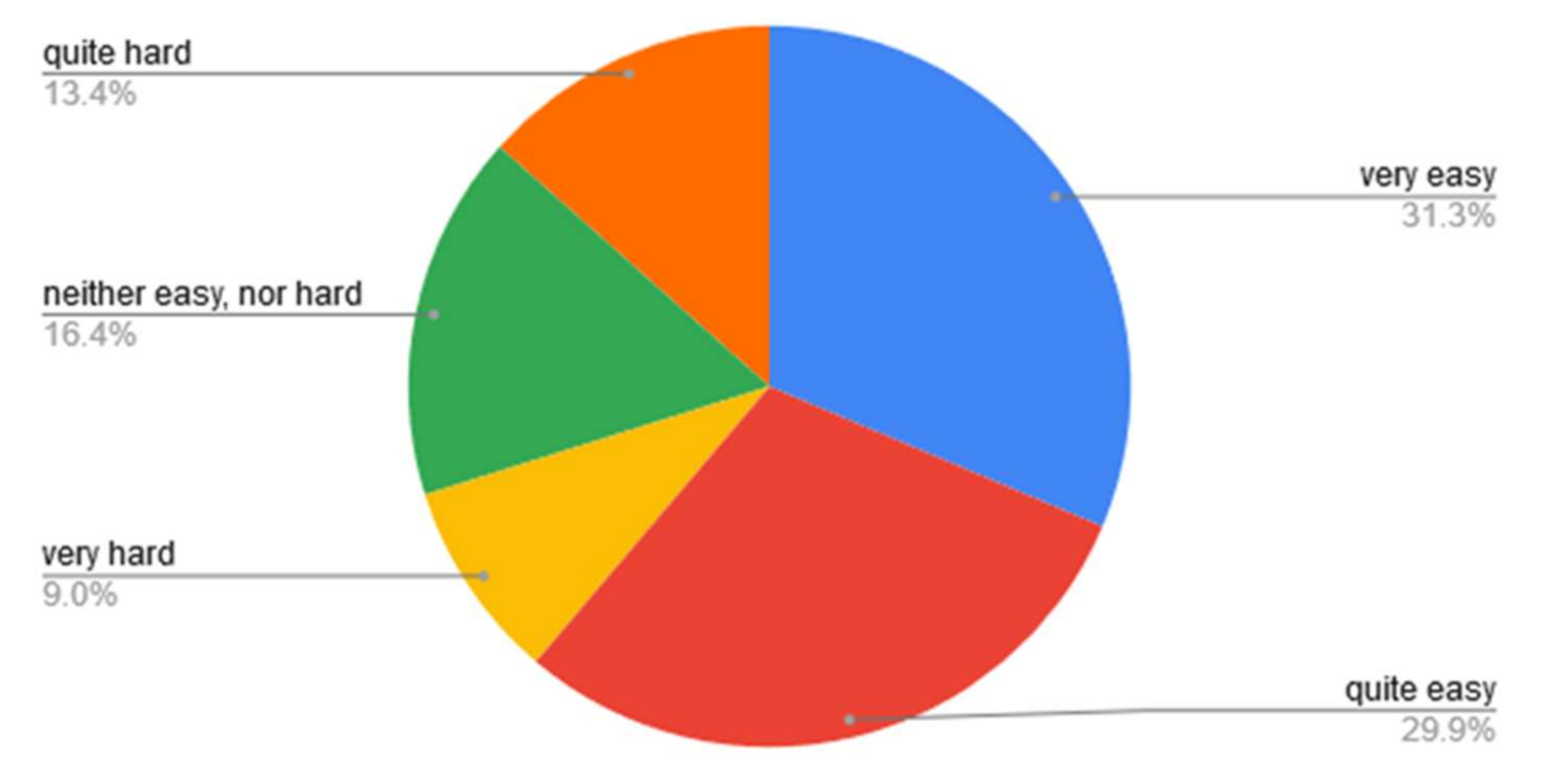
Figure 1, answers related to how hard it was for the test participants to tell if they were extraverts or introverts are presented.
Figure 2 shows the percentage of votes on a music genre which were given by introverts and extraverts. Based on the survey results, it may be said that most of the participants did not have much problem in identifying their personality traits. We can also see that in this age group, all music genres are listened to by both extraverts and introverts. However, among the music genres analyzed extraverts rather than introverts liked techno and house in the majority.
Based on collected results, each music piece in the dataset was given a score, which we called the personality advantage metric (PAM). It was calculated according to the following formula:
where:
denotes the number of extroverted participants who liked given musical excerpt,
denotes the number of introverted participants who liked given musical excerpt,
denotes the total number of extroverted participants taking part in the study,
denotes the total number of introverted participants taking part in the study.
Five surveys for five groups of people were performed, and each of them had different numbers of introverted and extroverted participants (
,
). The exact number of both classes of participants is given in
Table 1.
The number of participants identifying themselves as introverts and extroverts is equal only in the case of surveys 1 and 4. Therefore, it is necessary to use the PAM metric that takes this fact into account and performs normalization by placing
and
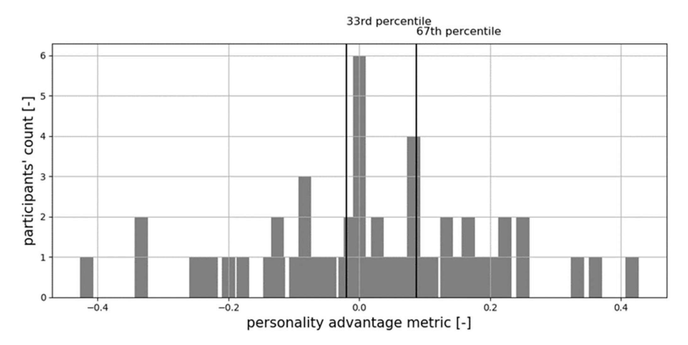
in the denominator of formula (1). The data obtained from the surveys were later used to determine if the given musical piece was more liked by people defining themselves as introverts or extroverts, and the ones for which no such relationship existed. To divide the presented musical excerpts into the three such categories, namely ones liked more by introverts, extroverts, and with no such preference, a histogram of the PAM metric was calculated. An example of such a histogram is presented in
Figure 3. This figure also has the 33rd and 67th percentiles of the PAM values denoted on the image. Those values were used to define the thresholds which separate the three ranges of PAM values, which we associate with musical pieces commonly chosen by introverts (I), ones more commonly chosen by extroverts (E), and ones preferred equally by both the extroverts and the introverts (N).
Each musical excerpt was assigned a letter denoting the set of PAM values it is associated with (I, E, or N). This label was later used to perform the classification process based on an objective parametrization of the musical signal and prediction with selected classifiers.
3.2.2. Musical Excerpt Parametrization
Parametrization aims at differentiating objects between different classes and determining whether an object is a member of a particular class. The need to parametrize audio signals stems from their redundancy. This process results in the creation of feature vectors containing between a few or a hundred or more parameters. Feature vectors are based on time-, frequency- or time-frequency-domain descriptors and are often completed by adding statistical parameters. These low-level features are usually derived from the MPEG-7 standard [
60]. However, Mel-frequency cepstral coefficients (MFCCs) as well as dedicated descriptors suggested by researchers in the music information retrieval (MIR) area are also widely employed [
22,
56]. Feature vectors may then be used in machine learning-based classification or clustering processes.
The same samples that were employed in the subjective tests (S set), and some additional ones from the extended dataset (ED) set, were gathered to constitute a database of 302 unique samples that were then parametrized by the use of MIRtoolbox [
56]. This toolbox contains approximately 50 parameters [
56], however, only several descriptors were utilized in the designed analyses. As already said, the significance of these parameters for a given music genre was checked by employing the statistical analysis carried out in our earlier study [
59].
They were as follows [
61]:
Root-mean-square energy (RMS energy) is a parameter describing the global energy of the signal. In audio segments, RMS represents the magnitude variation over time, and it may be helpful to separate silence and audio signals;
The zero-crossing rate is a parameter related to the physical properties of the waveform. It is related to the noisiness of the signal and shows how many times the signal crosses the X-axis. It can also be useful for measuring the dominant frequency in the signal and finding a discriminator for speech/musical signals;
Spectral centroid, which returns the first moment called the “mean”, is also the geometric center called the “centroid”. It is a measure of the center of gravity called “brightness”;
Spectral skewness represents the third central moment. It shows to what extent the distribution is asymmetric around its mean. A positive value of this parameter signifies that the distribution has a longer tail to the right; a negative value means the opposite. The symmetrical distribution has a value equal to zero;
Spectral kurtosis is the fourth standardized moment minus three, which is a correction of the kurtosis of the normal distribution equal to zero. It shows the flatness of the spectral distribution around its mean;
Spectral flatness which represents the ratio of the arithmetic and geometric means of the coefficients of the power density spectrum in all spectral bands (b) of 1/4 octave width. It is also called the “tonality coefficient” [
62];
The entropy of the spectrum is a measure of spectrum uniformity, which refers to the relative Shannon entropy;
Roll-off is a measure of spectral shape. It returns the frequency boundary value below which 85% of the total power spectrum energy is concentrated.
The above-cited parameters were checked as to their significance for a given music genre by employing the statistical analysis.
3.3. Parameter Analysis in the Context of Music Genres
The statistical analyses of the MIRtoolbox parameters given in the context of music genres showed that there were statistically significant differences between the main genres, sub-genres, and mixed genres. Features derived from the MIRtoolbox software may be treated as factors influencing the assignment of a given musical piece to a particular genre. Our primary focus was the prediction of personality types associated with the majority of the given musical excerpts. However, we also wanted to test if parameters we were investigating for such a purpose could be used to distinguish between music genres. The ANOVA test was performed to find out which of the utilized parameters differed in a statistically significant manner if music excerpts were divided into genre-related groups. Parameter values were averaged for the whole musical excerpt. For calculation, an implementation of the ANOVA test available in the R language standard library was used [
63]. The results of this analysis are shown in
Table 2.
Table 2 contains the F statistic associated with each analyzed parameter. Moreover, the
p-value associated with a particular value of the F statistic is provided. From nine investigated parameters, four of them were found to be statistically significant in terms of separation between music genres, i.e., RMS, zero-crossing rate, spectrum centroid frequency, and spectrum skewness (highlighted in
Table 2). The level of significance in the case of the abovementioned parameters is 0.001.
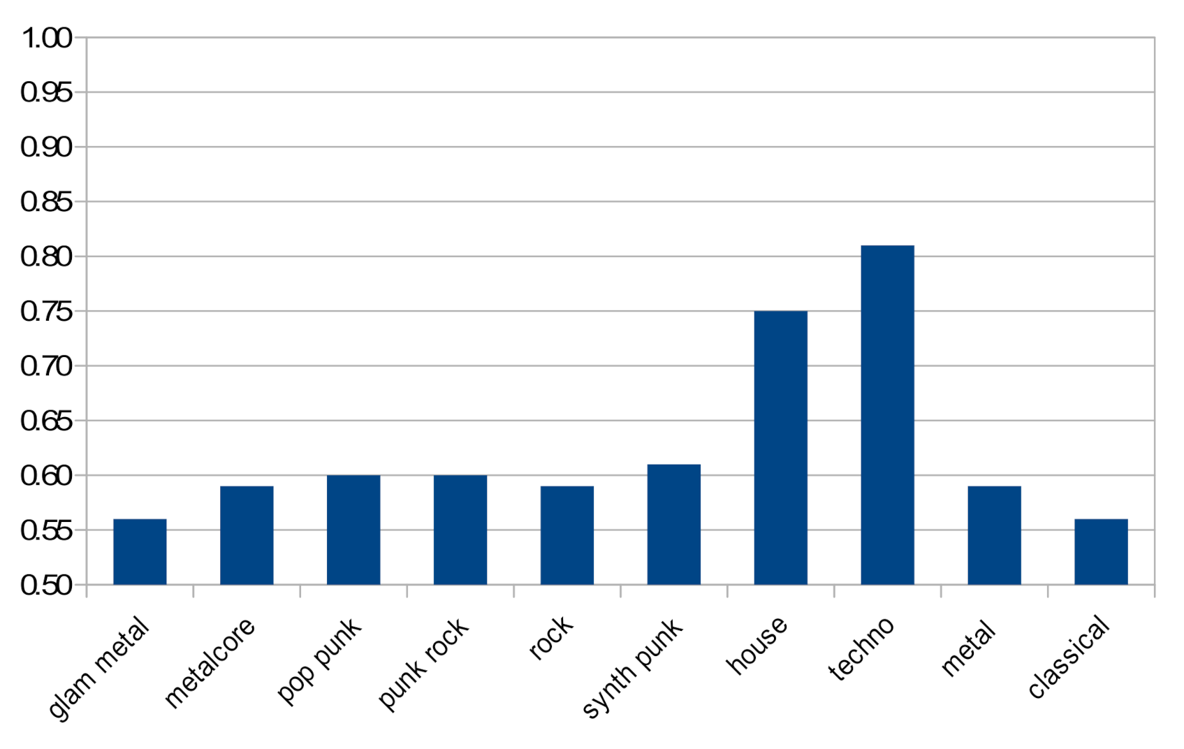
To show the variability of given parameter values between music genres, the RMS descriptor was used, see
Figure 4. For instance, house and techno, which belong to electronic music, have much higher RMS energy than the others (including electronic punk known as synth-punk). In addition, it can be observed that the punk and metal music genres share many characteristics with rock music that differ from electronic or classical music. Rock, metal, and punk have low mean values of RMS energy. The mean values of the electronic genre are much higher.
However, as the music genre classification is not the primary aim of the paper, we decided not to restrict a set of parameters analyzed in this subsection to the only ones which provided a statistically significant distinction between genres. Therefore, all of the aforementioned parameters were calculated for music excerpts analyzed in the further analyses focused on the prediction of the listeners’ personality type.
3.4. Variational Autoencoder Neural Network-Based Parametrization
It should be mentioned that there were two sets of music used in the experiments. The set employed for the surveys (S) contained musical pieces other than the ones fed into the machine learning algorithm. The latter one is called the extended dataset. However, both of them were derived from one joint dataset, thus they contained the same music genres. This was to provide additional music excerpts for training and validation processes, fed into the input of one of the benchmarked parametrization algorithms [
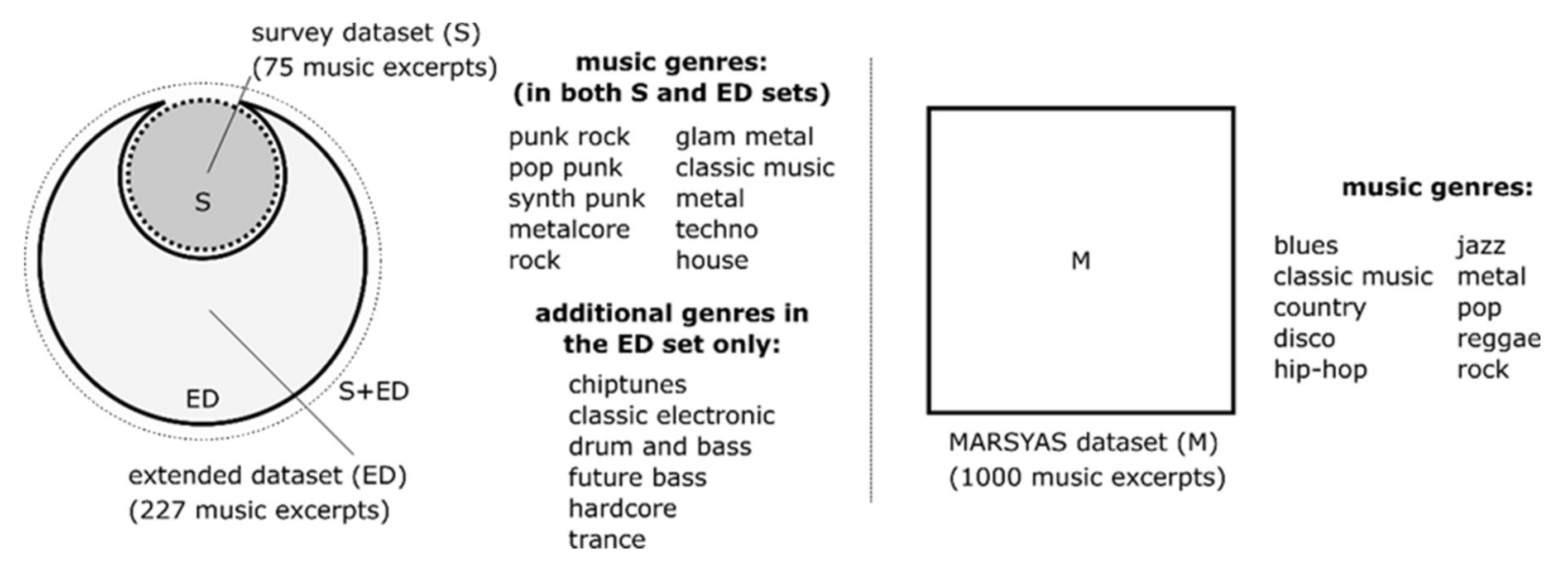
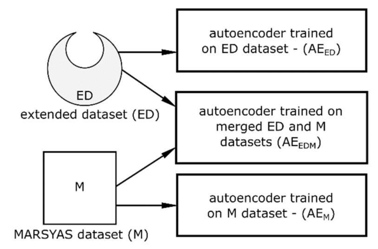
64]. Besides, in the case of a variational autoencoder neural network-based parametrization, the MARSYAS (M) dataset was also used to augment the training dataset. The M dataset contained music of other genres than S and ED datasets. It was used to find out if augmentation of the input dataset with more music examples of genres different than ones used initially in the survey influenced the performance of the baseline classifiers employed in the next step of the experiment. A graphical depiction of all used datasets is provided in
Figure 5.
As already mentioned, the dataset S was used as the audio material in the surveys. Surveys were utilized to derive ground truth labels. Musical excerpts from the dataset S and the survey-derived labels denote if a given musical excerpt from the S dataset was preferred by introverts, extroverts, or there was no such a preference. The labeled dataset obtained in such a way was then treated as a benchmark dataset for evaluation of the performance of the classification algorithms. It is the only labeled dataset used in the study, the remaining two datasets (namely ED, and M datasets) were used for unsupervised training of the variational autoencoder. The number of musical excerpts in each dataset and the genre composition of ED and S datasets are shown in
Table 3.
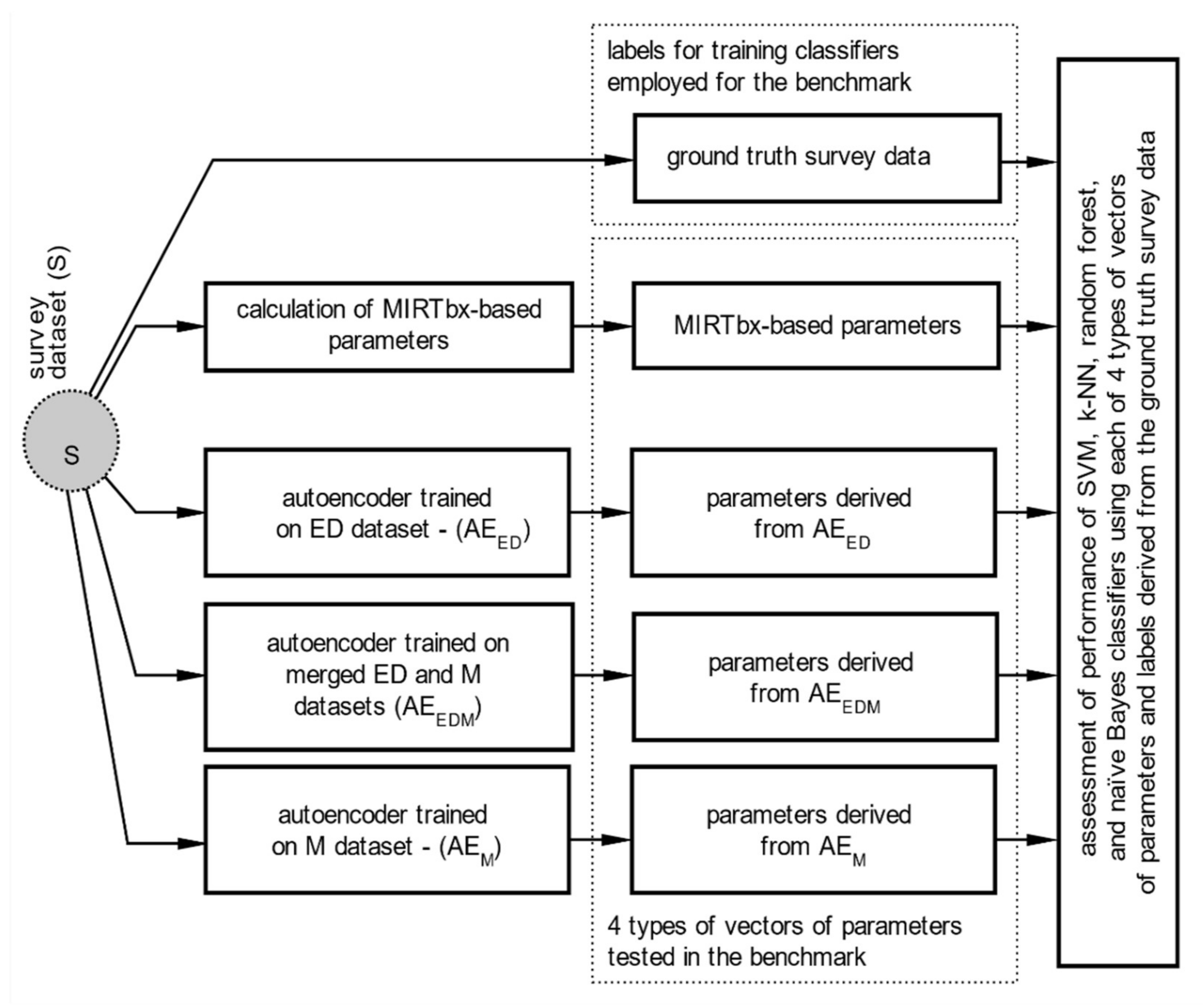
Classification of the musical excerpts from the set S was performed in four ways. The first one was a simple parametrization based on MIRtoolbox [
44]. The second one concerned a parametrization approach using a variational autoencoder neural network but different input dataset configurations. First, the autoencoder (AE) was trained only on the ED dataset (AE
ED) containing musical pieces belonging to the same genres as the S dataset. Then, a neural network of the same architecture, as in the above case, was trained on the M dataset (AE
M). The third autoencoder was the same as the first and the second ones but trained on the sum of the ED dataset and the M dataset (AE
EDM). The process of the autoencoder training is illustrated in
Figure 6, and the whole experiment scheme is provided in
Figure 7.
The parametrization and prediction stages were separated because our intention was to investigate how different choices of training samples influence the quality of parametrization based on autoencoder neural networks. Similarly, we would like to find out if including samples from a dataset that has a different genre structure (M dataset) when compared to one having a similar genre structure to the dataset used for the surveys changes the classification outcome. The reference method for this comparison was parametrization based on the MIRtoolbox parameters. The quality of the parametrization was assessed by performing a classification task with a set of selected machine learning classifiers. The implementations of the algorithms are based on the Python machine learning library called Scikit Learn [
65].
As already stated, four types of classifiers were employed: SVM, k-NNs, RF, and NB. Each of the aforementioned classifiers takes an MFCC-gram derived from a given music excerpt and predicts the type of listeners who would like this excerpt. Each excerpt is assigned to one of the three groups derived from the PAM metric obtained from the survey data (namely I, N, or E group).
The following sets of hyperparameters were used for each of the baseline algorithms employed:
SVM—a nonlinear version of the algorithm was used, kernel was set to radial basis function (RBF), γ = 0.14; C = 250,
k-NNs—k was set to 8,
RF—the minimum number of samples required to split an internal node (min_samples_split) was set to 15, the maximum number of features taken into account when looking for split (max_features) was set to 34, and the number of trees (n_estimators) was set to 35,
NB—a Gaussian NB implementation of the algorithm was used.
The default values were used for all other hyperparameters as prescribed by the Scikit Learn library (version 0.21.3).
The data parametrized with the MIRtoolbox were designed to contain temporal information as this can also carry information associated with the music genre or the probability of invoking a certain mood in a listener. For the parametrization, we extracted 20-s excerpts of an audio signal from all of the pieces of music used in the study. This was then split into ten 2-s-long frames and five 4-s-long frames. Each frame was used to derive nine averaged parameters which are implemented in the MIRtoolbox software. We computed the RMS power, and the zero-crossing rate for the time-domain. On the basis of the spectrum of the frame, we calculated its centroid, skewness, kurtosis, flatness, entropy, brightness coefficient, and roll-off. Each computation resulted in one scalar value, which was associated with the whole 2-s or 4-s-long frame. Thus, we obtained 45 parameters for the scenario employing 4-s-long frames and 90 parameters if 2-s-long frames are considered.
Next, parameters from a neural network calculation process were derived. To carry out such a parametrization, we used a variational autoencoder neural network. One of the features of such networks is that, unlike regular autoencoders, they generate embedding space, which has no areas with no association to the items that they encode. In our case, the encoded items were MFCC-grams of the 20-s musical excerpts, the same that were parametrized earlier with the use of MIRtoolbox.
To take into account two frame lengths employed in the case of MIRtoolbox, we trained the autoencoder, which performed encoding into a 45-dimensional space and one encoding example into a 90-dimensional space. As a result of this, the effects of the MIRtoolbox-based and autoencoder-based parametrization will be comparable as the length of the encoding will not impact the possible efficiency of the algorithms utilizing the same length of the vector of parameters.
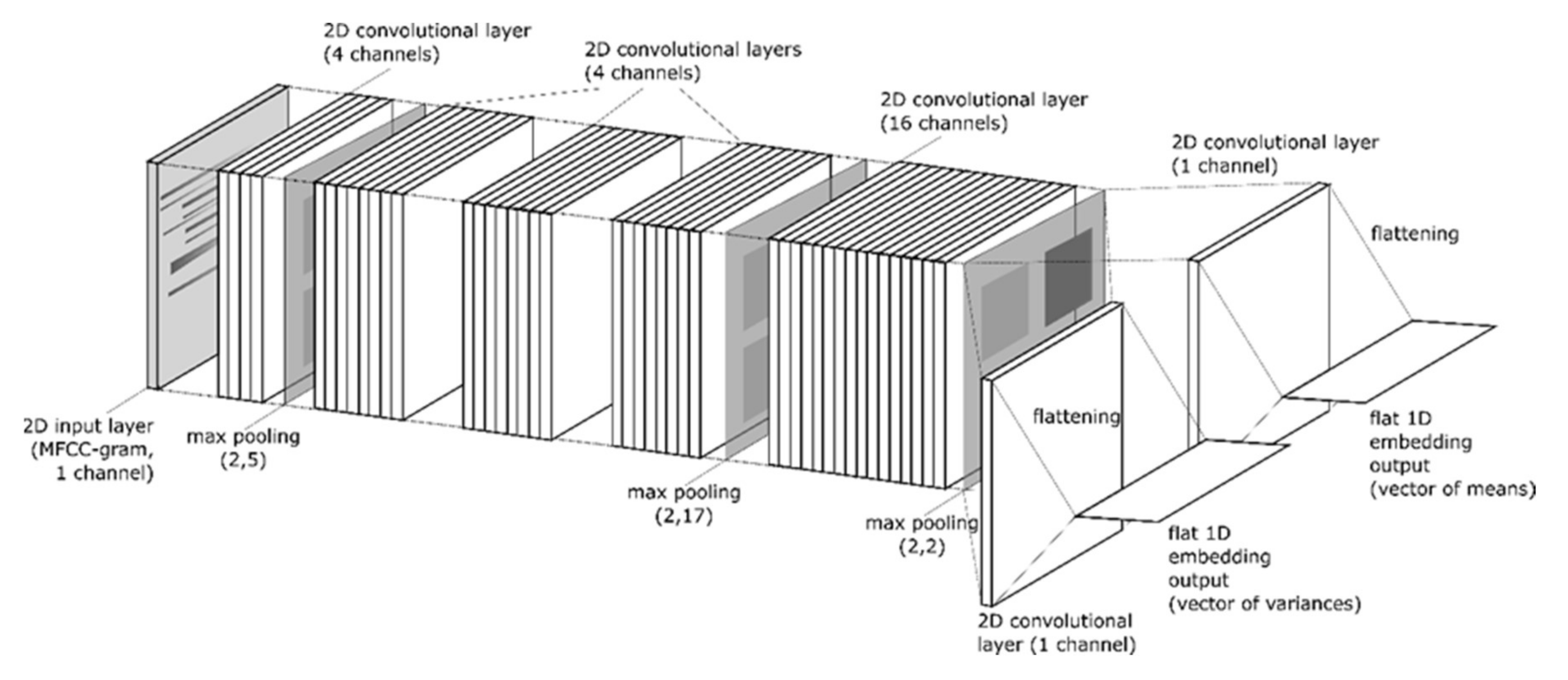
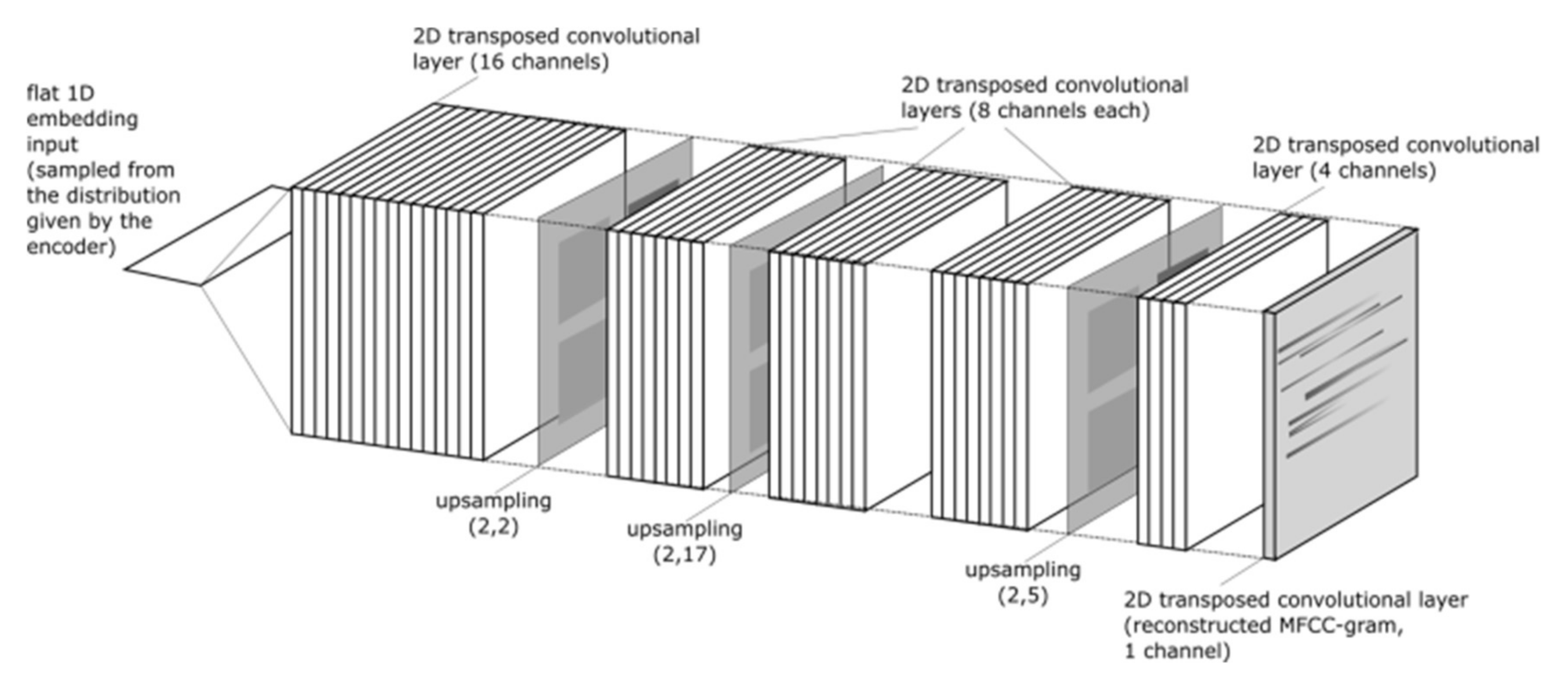
The structure of the encoder neural network used in our study is provided in
Figure 8. The structure of the decoder neural network utilized is provided in
Figure 9.
The parametric rectified linear unit (PReLU), which could be optimized in the process of the neural network training was employed as the activation function of the convolutional layers in the case of both the encoder and decoder. Each convolutional layer used the convolutional kernel size of (3,3). As an optimizer, an ADAM (ADAptive Moment estimation) algorithm was employed. The initial learning rate of the optimizer was set to , and the other parameters were set to their default values assumed by the Keras API (Application Programming Interface) used for the implementation of the neural network.
Additionally, a dropout procedure was applied during the training phase to each output vector of parameters returned by the encoder neural network. The rate of the dropout was set to 0.2, which means that 20% of parameters were randomly set to zero in each epoch. The reason for the use of a dropout procedure is to enforce the variational autoencoder algorithm to generate representation vectors that allow reconstructing the original encoder input even if there is missing information in the vector of parameters. Thus, the algorithm cannot simply depend on a set of a few parameters to achieve high low reconstruction errors and has to make the use of the embedding space (namely, all 45 or 90 parameters depending on the frame length) as any element of the vector of parameters has a chance to be randomly set to zero during the training phase.
The training duration was 500 epochs for each of the autoencoder neural networks employed in the study. The final loss value from the last iteration of the training process was similar in all cases and was in the range of between −2856 and −3407. In the case of training the autoencoder with 45-dimensional latent space on the E set, we had to restart the training procedure once. This was necessary because the algorithm was stuck in the local error function minimum; the loss value, in that case, was close to −1000. A restart of the training allowed the algorithm to reach a value of loss equal to −2856, which was closer to the outcomes observed for the rest of the algorithms. The MFCC-grams used in our study consisted of 510 frames containing 120 MFCC parameters. Such a choice of dimensions was imposed by the requirement to obtain autoencoders generating embeddings that have a length of 45 and 90 parameters. To achieve this goal, the original dimensions of MFCC-gram must allow their reduction by pooling in such a way that a resulting feature map contains 45 or 90 parameters. For example, if the resulted embedding has a length of 45, we can reduce the size of (120,510) to (15,3) by the max pooling operations depicted in
Figure 8. After the flattening operation, the layer having a shape of (15,3) results in an embedding of 45 parameters. Thanks to the fact that the reduction of the size was always by an integer factor, the original sizes of the feature maps can be retrieved in the decoder by an upsampling procedure, which can only increase the size of the feature map dimension by an integer factor.
4. Personality Type Prediction
To assess if the parameters obtained from both the MIRtoolbox and autoencoders can be applied to predict the personality type of persons who listen to musical excerpts encoded by them, we performed a benchmark test. The benchmark consisted of training four simple classifiers, i.e., SVM, RF,
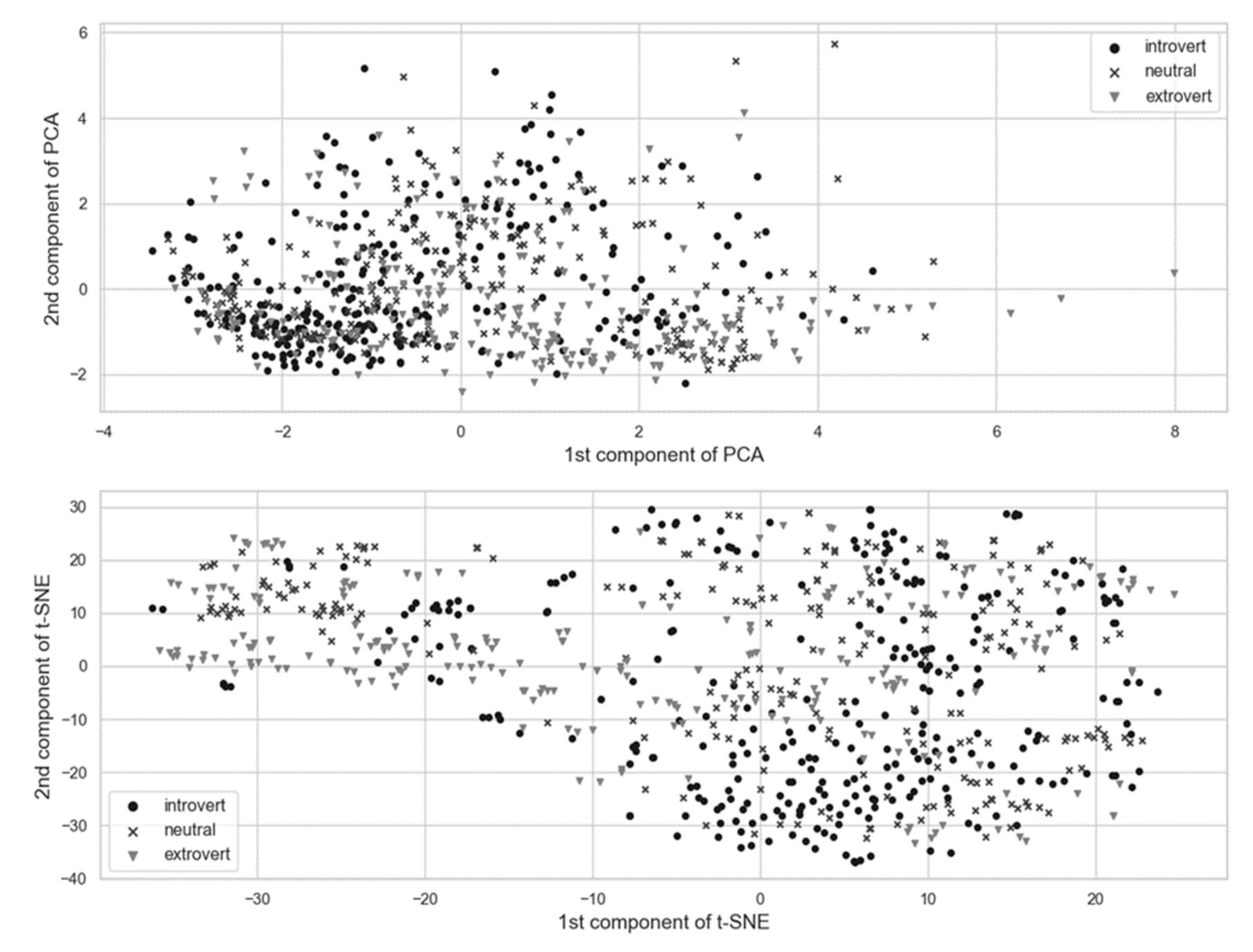
k-NNs, and NB classifiers on the parameters obtained from the S set. As previously mentioned, this is a set for which we obtained labels indicating if the musical excerpts belonging to the set were preferred by extroverts, introverts, or if there was no preference. It contained 75 fragments of musical pieces, and each personality preference class consisted of 20 examples. This number is small, thus for the analysis, we employed not only fragments that were presented to the participants but all possible fragments which could be derived from all the audio material. Recordings of musical pieces were split into 20 s-long frames with a 10-s margin between consecutive frames. The gap between frames allowed for obtaining frames, which were likely less correlated with each other, and thus can further improve the performance of the classifiers employing them as their input. Due to such an operation, we obtained 752 frames. Each frame was assigned one of three labels denoting if it was mostly preferred by introverts (consisted of 288 frames), extroverts (consisted of 237 frames), or if there was no preference (consisted of 234 frames). The number of samples in each group was equal (230 samples per group). For evaluation of performance, we employed 5-fold cross-validation, which was repeated five times with a random assignment of examples into each fold. This yielded 25 observations for each pair of classifiers and types of parameters. An example of visualization of the latent space generated by MIRtoolbox-based parameters is provided in
Figure 10. As the 45-parameter dataset performed slightly better, that is why this dataset was chosen for 2D visualization.
The dimensionality reduction techniques used for visualization were primary components analysis (PCA) and t-distributed stochastic neighbor embedding (t-SNE). The first one is a standard method for visualization of high-dimensional datasets in 2D and 3D visualizations. The latter approach is a nonlinear technique [
66], and as such does not preserve actual distances from the high-dimensional latent space it visualizes, but it retains the neighborhood relation of the data points. It was also possible to visualize latent space generated by the variational autoencoder. In this case, the best performing parameterization method (in terms of maximal achieved accuracy) also used 45-dimensional space. It resulted from training the autoencoder on both the ED and M datasets. The resulting latent space is visualized in
Figure 11.
Using a variational autoencoder enabled us to treat the distance between the points as a similarity metric, which is not the case if regular autoencoders are considered. It should be noted that in the case of variational autoencoder separation between the personality preference group can also be seen using much simpler visualization based on PCA. Thus, we hypothesize that this feature may help other algorithms employing parameters calculated by the variational autoencoder to classify not only the music genre but also to predict the most probable personality type of a listener interested in each parametrized musical excerpt.
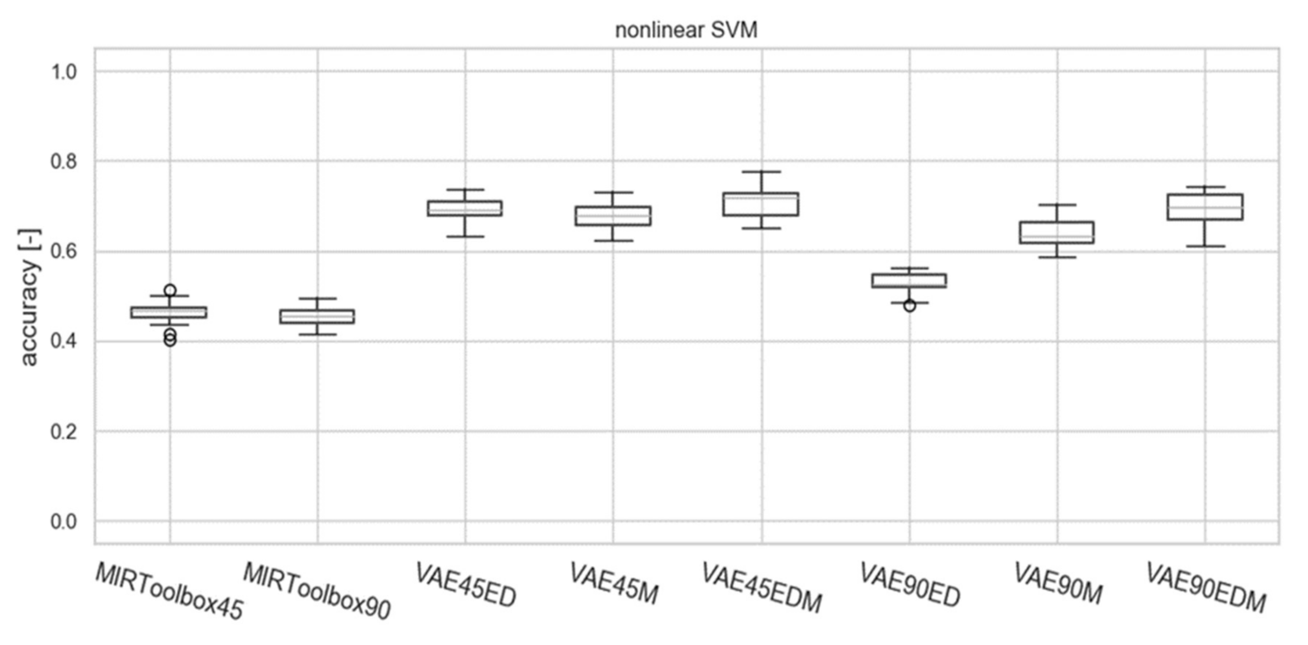
For the SVM algorithm, a boxplot showing the structure of the obtained results is depicted in
Figure 12. Parameters calculated with the use of MIRtoolbox are denoted as “MIRTbx”, ones obtained with the use of a variational autoencoder start with the “VAE” prefix. Furthermore, the number of parameters is specified (namely 45 or 90). Finally, in the case of the autoencoder-derived features, a training dataset is named. Autoencoder trained on the extended dataset is marked by a letter ED, one trained on the MARSYAS dataset is denoted by M, and EDM means a sum of ED and M sets. This naming scheme will also be used in further figures and tables, which contain the results of the performed analyses.
The Levene test was first performed for all tested algorithms to find out if the use of the ANOVA test found the statistical significance of the observed differences. In the case of all classifiers but the SVM classifier, the Levene test returned
p-value lesser than
, which means that variances of observed dependent variables are equal, and thus the requirement of homoscedasticity imposed by the ANOVA test was not satisfied. However, in each algorithm, at least one variable did not have a Gaussian probability distribution, which was tested with the Shapiro–Wilk statistic test. The test was repeated for each dependent variable and then corrected for multiple testing. Such a procedure was repeated for a set of results obtained from each classifier separately. Such outcomes of initial statistical testing meant that we could test the significance of differences between the performance of each classifier with different parameters set with the Kruskal–Wallis test which is a nonparametric alternative for the ANOVA test. For the SVM classifier, the Kruskal–Wallis test yielded a test statistic of 163.76, and thus its
p-value was less than
, which allowed us to conclude that at least one pair of variables from
Figure 12 have medians, which were different in a statistically significant way. To determine which differences were significant, we carried out Dunn’s post hoc test and obtained the results shown in
Table 4. It is worth noting that the autoencoder based parameters performed better than any parameters derived from the MIRtoolbox software. Similarly, the VAE45 EDM dataset achieved performance statistically similar to ones obtained from single-dataset parameterization methods consisting of 45 dimensions. It also was performing similarly to the analogous parameter set consisting of 90 dimensions.
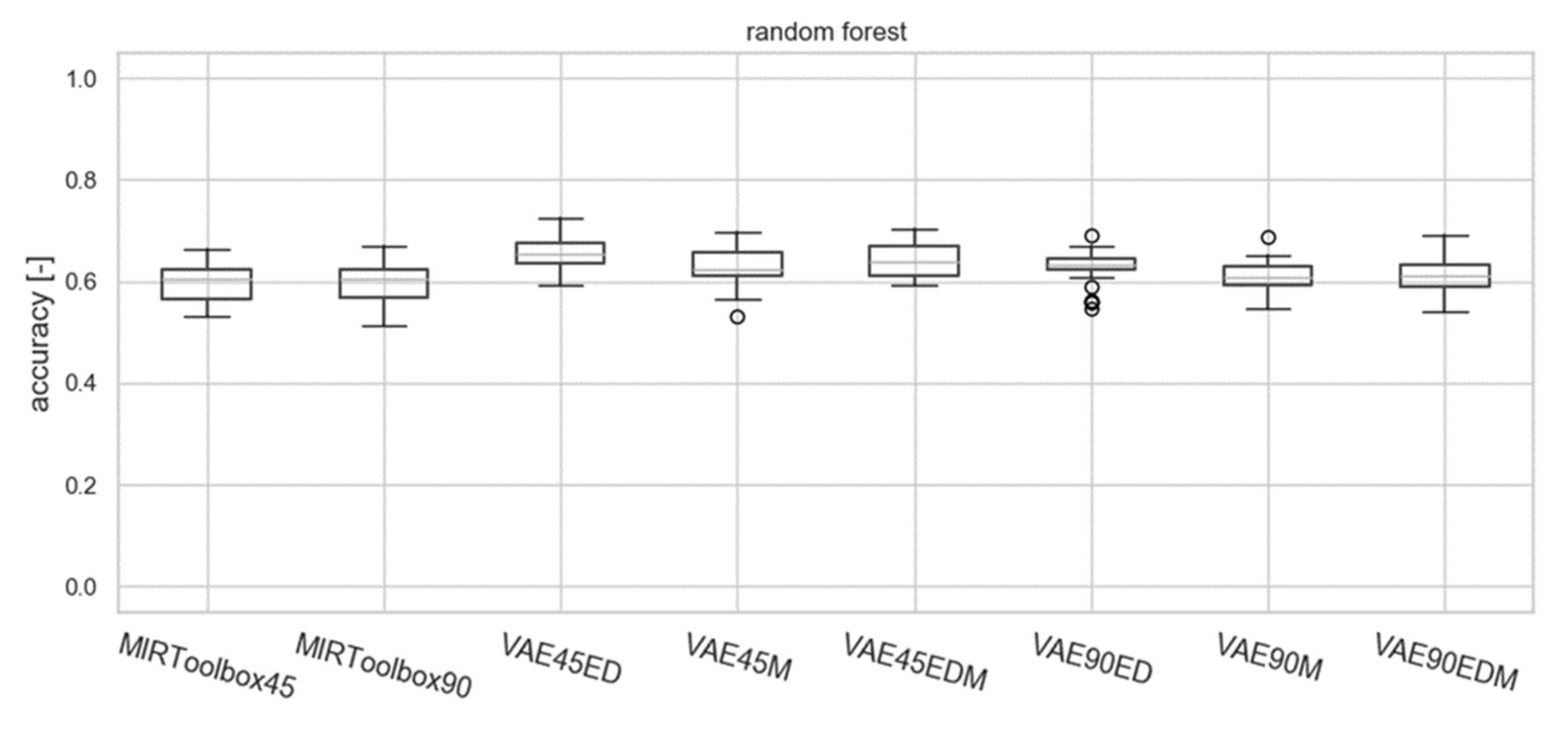
In the case of the RF classifier, we obtained a Kruskal–Wallis test statistic with a value of 41.01, and thus the
p-value was less than
. This meant that we could apply Dunn’s post hoc test, as there were significant differences between the variables in
Figure 13. The matrix of
p-values resulting from this test is shown in
Table 5.
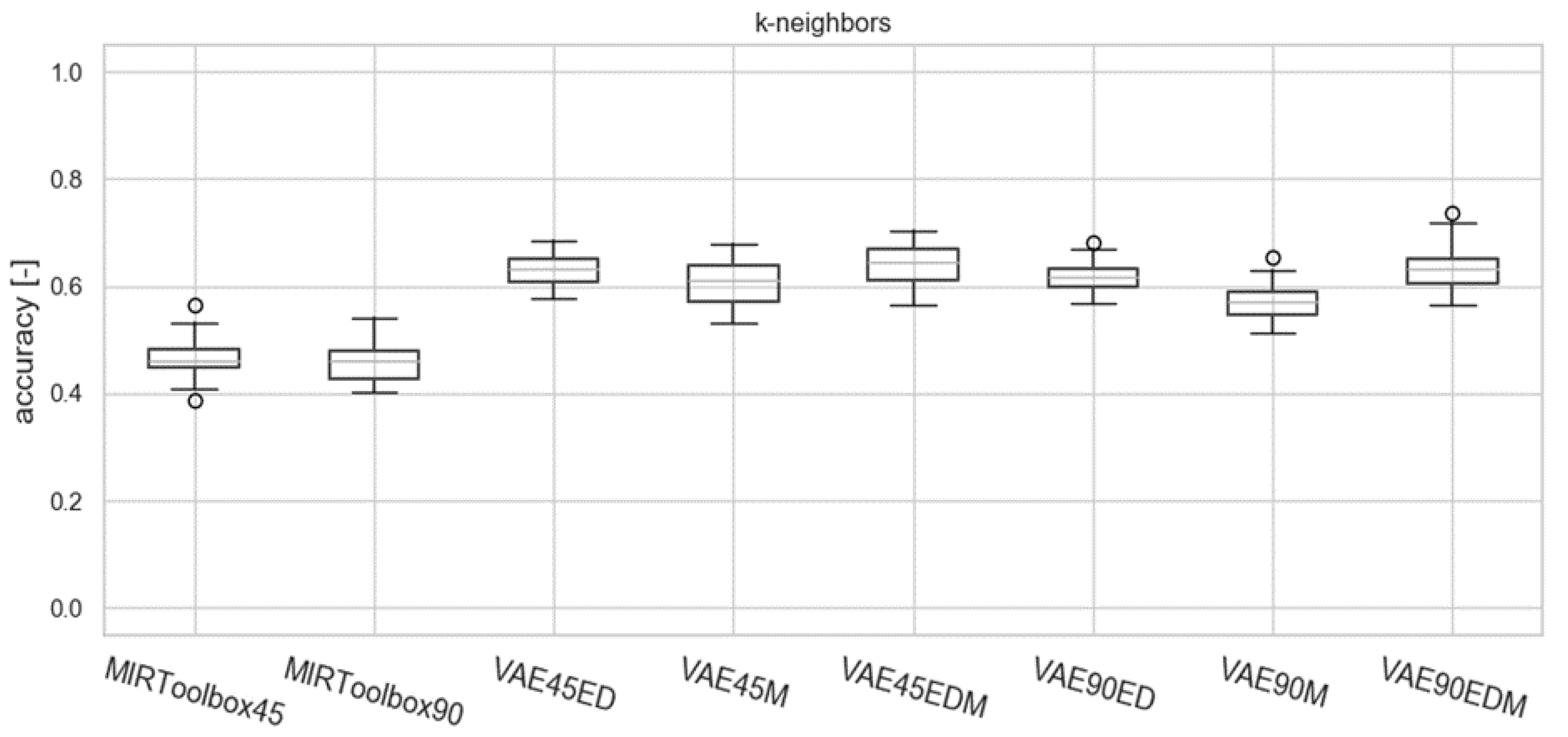
For the
k-NN algorithm, we obtained the following results. The statistic of the Kruskal–Wallis test was equal to 134.20, and the
p-value was less than
(see
Figure 14). Therefore, we could carry out Dunn’s test, and the resulting matrix of
p-values is shown in
Table 6.
The last algorithm tested in our study was the NB algorithm for which the results are shown in
Figure 15.
The statistic for the Kruskal–Wallis test in the case of the NB algorithm was equal to 45.55, and therefore the
p-value of this test was also less than
. The
p-values associated with Dunn’s post hoc test can be found in
Table 7.
It should be noted that two of the investigated classifiers performed poorly and did not benefit from parameters obtained from the variational autoencoder—namely the RF and the NB classifiers. The k-NN classifier was able to benefit from parameters generated through the machine learning algorithm, which we hypothesize, is probably a consequence of the principle of operation of the variational autoencoder, as it tends to generate closer embeddings (in terms of Euclidean distance in the high-dimensional space). However, the k-NN algorithm was still outperformed by the nonlinear SVM algorithm, which suggests that some additional information can still be extracted from the embeddings generated by the variational autoencoder.
In the case of k-nearest neighbors and the SVM algorithm, we also observed a statistically significant increase of the accuracy values. The best median accuracy was achieved by the SVM classifier using parameters from the VAE45 EDM scenario. The median of obtained accuracies, in this case, is equal to 70.96%.
5. Summary and Conclusions
The study aimed to investigate if it is possible to predict the personality trait of potential listeners on the basis of a musical excerpt by employing two types of parametrization, i.e., based on MIRtoolbox and a variational artificial neural network and several classification algorithms. First, listening surveys were conducted to explore the kind of music preferred by extraverts and introverts. This was also a way of gathering ground truth information for the classifiers.
It is essential to observe that there are differences between the declared choices of the extraverts and introverts. However, this observation only partially agrees with the results shown in the literature. Additionally, it may be relevant that the declared extraverts were choosing many more excerpts than the introverts. Even more important is the fact that the respondents were not asked about their favorite music genre/s but the music they enjoy listening to. These observations only partially agree with the results shown in the literature. Furthermore, many of the music genres which we chose are grouped in those studies (e.g., punk rock, pop-punk, synth punk, and metalcore). That is why it is not possible to thoroughly compare the results to other works results as we used music genres rather than music description. However, some of the results obtained can be observed in the context of other works.
Most people listen to more than one music genre and may not even have a favorite genre, so asking people to choose music excerpts they enjoy seemed more suitable for the research. Most of the votes given on punk rock belonged to extraverts, however, the scores assigned to music genre by extraverts and introverts were in the proportion of approximately 53%/47%. This does not correlate with the result obtained by authors of one of the studies, which stated that punk was preferred by introverts [
38]. Moreover, neither of the sub-genres or mixture of genres, including punk music (pop-punk, synth punk, and metalcore), was chosen by majority of introverts. In the case of rock music, which was supposed to be chosen by the introverts [
37] or mainly by them [
38], rock music was also much more often chosen by extraverts. Metal music was supposed to be chosen mainly by extraverts [
38], and this agrees with our results. In contrast, there is a vast difference between votes given on a genre by extraverts and introverts. Classical music was supposed to be chosen mainly by introverts [
38], which corresponds to some extent to our results. However, classical music is the only genre where the majority of the votes given on the specific genre belonged to introverts. Electronica was said to be chosen mostly by extraverts [
44]. So was pop/dance [
37]. In our study, electronic music was presented by two subgenres: Techno and house, and a mixture of punk and electronic music called synth punk. All of them were chosen mostly by extraverts. It is visible in the case of techno and house rather than synth punk. Pop music was considered either along with dance music (preferred by extraverts [
44], or alone and also liked mostly by extraverts [
38]. In our study, the only genre related to pop music is pop-punk, which was also mostly chosen by extraverts.
The results of the statistical analyses shown in the previous section led to the conclusion that autoencoder-based features of musical excerpts were, in general, more likely to carry useful information associated with the personality of the potential listeners than the parameters derived from the MIRtoolbox. We also found that training of the autoencoders on sets of musical pieces which contain genres other than those employed initially in the survey in most cases did not affect the accuracy of the classifiers predicting the personality of the survey participants. The best result was obtained for the SVM classifier utilizing the embeddings with a length of 45 parameters. The maximum accuracy of prediction reached 78%. However, it is important to note that this was the highest achieved score. The typical value of accuracy in this case, which is represented by the median, was equal to approximately 71%, which is still a satisfactory result, especially if taking into account the fact that the autoencoder was not provided with the context of the personality prediction task and was only analyzing the musical signal in an unsupervised manner.
As already said, it is difficult to compare the results obtained to other works as the assumptions, methodology, and settings designed by other researchers differ from our experiment. For example, Feiereisel and Quan showed that preferred music genres could be predicted from hobbies and interests with an accuracy of 58%. Schulte [
30] got similar results with several classifiers (e.g.,
k-NN returned accuracy of 0.48, linear SVM 0.54, whereas nonlinear SVM got 0.52). Predictive accuracies obtained by Nave et al. [
43], presented as the Pearson’s (
r) correlation between the actual and predicted personality-trait scores (above the general baseline model), were highest for openness (Δ
r = 0.09, 55% increase) and extraversion (Δ
r = 0.08, 79%). These values were less pronounced for the three other traits, namely neuroticism (Δ
r = 0.03, 17%), agreeableness (Δ
r = 0.02, 15%), and conscientiousness (Δ
r = 0.01, 7%) [
43].
Even though the assumptions and conditions of our study differ from other research works, we can conclude that the outcomes of our research are similar or better compared to the state-of-the-art.
The autoencoder-based approach for music signal parametrization may be useful in fields such as audio music branding, i.e., to encourage a certain type of customers to purchase their products in a given place. Such an analysis may be performed just by utilizing the features calculated from audio samples of the music. The observation from our study shows that such a way of extracting parameters enhances the performance of simple classifiers such as SVM, or nearest-neighbor algorithms, making it a possible direction for future research.
Therefore, one may assume that such a methodology may be helpful to match the preferred kinds of music to the listener’s personality. However, it should be mentioned that choosing the extraversion/introversion option was left to the respondents to decide. We assumed that the understanding of the personality traits was sufficiently clear to them as the definitions of extraverts and introverts were included in the survey. The results reported on to what extent it was difficult to assign oneself to a given personality trait showed that in the majority of cases, this was not a problem. However, in the future, all subjects may also be briefed as to what being an introvert, or extravert entails.
