Abstract
A model-independent control strategy called high-order differential feedback control (HODFC) is applied to a quadrotor unmanned aerial vehicle (QUAV) based on a semi-autopilot indoor optical positioning system. The affine system form of the quadrotor model is provided to facilitate the design of the HODFC. A fifth-order high order differentiator (HOD) is introduced to estimate with high precision the derivatives of the reference input and the QUAV system’s states. A filtering signal of the control output is incorporated in the control law to overcome the system model’s unknown part in the HODFC scheme. The stability of both the HODFC and the HOD are proved. The physical and straightforward parameters are provided to make the HODFC scheme for the QUAV easy to operate. The real-time trajectory tracking experiments with varied reference trajectories and disturbances are carried out to illustrate the superior performance of the HODFC versus the proportional-integral-derivative (PID) method, in terms of the mean of absolute error, the integral of absolute error and the integral of the time-weighted absolute error. The results also demonstrate that the HODFC has superiority in static and dynamic trajectory tracking, especially when the system is disturbed.
1. Introduction
Quadrotor flying platforms are a class of unmanned aerial vehicles (UAVs) that have been widely applied in exploration [1,2], transportation [3], cooperative pursuit [4], and so on. It is challenging to design a reliable controller for quadrotors because of their under-actuated, nonlinearity, strong coupling, static instability and abundant dynamic behavior in the attitude system [5]. At present, the control strategies applied to the quadrotor are mainly divided into model-dependent control and model-independent control [6]. Model-dependent control mostly requires knowing the exact mathematical model of the system. The sliding mode control (SMC) is a typical method based on the system model. Mu et al. [7] investigated a novel integral SMC strategy for waypoint tracking control of a quadrotor. Tian et al. [8] proposed a multivariable super-twisting-like algorithm for arbitrary order integrators. A robust nonlinear control method was provided by Liu et al. [9] with the quaternion representation. The problem is that in actual engineering, the accurate mathematical models of the systems cannot be obtained because of the unmodeled dynamics, uncertainties and unknown disturbances, such as wind disturbance, actuator failure and configurations of bobweight. These factors make the model-dependent control algorithm more complicated and challenging to apply and popularize in practical engineering.
The classic PID controller is a typical model-independent control. Salih et al. [10] designed a PID controller to realize the steady flight of a quadrotor in 3D space. Salvador et al. [11] optimized the PID parameters by a nonlinear scheme to reduce the steady-state error. With the development of the related theory of intelligence, many new controllers were designed, such as the expert system PID controller [12], the fuzzy PID controller [13] and the neural network PID controller [14]; these overcome the deficiency of the classic PID controller and achieve a better control effect. Another popular model-independent control strategy is active disturbance rejection control (ADRC), which was proposed by Han [15] and modified by Gao using a linear form [16]. The ADRC has significantly contributed and enriched control theory in terms of anti-disturbance and application when there is an unknown model. It has been successfully applied to some industrial control processes [17,18]. The ADRC usually uses the extended state observer (ESO) to estimate model function, and then a stable closed-loop system based on the ESO is designed [19]. Zhao and Guo [20] established conditions that guarantee the ADRC achieves closed-loop system practical stability, disturbance attenuation, and practical reference tracking. Yang et al. [21] designed an inner-loop controller with the ADRC method and analyzed the quadrotor’s stability under gust wind conditions. Li and Chen [22] designed a reduced-order ADRC; simulation and Qball2 platform experiments were carried out to verify the effectiveness and superiority of this method. Chen et al. [19] summarized the latest research progress of ADRC in theory and application in recent years and made a prospect for subsequent research.
In addition to the above control methods, another model-independent control called the high order differential feedback control (HODFC), based on the high order differentiator (HOD), was proposed by Qi et al. [23,24]. The HODFC method only utilizes the output and reference input of the system. The HOD was designed to estimate the different order differentials of the input and output signals of the system. These extracted derivatives of output are observed states of the system, so they are essential information. The HODFC uses the different orders of derivative errors of the given input and output to design a pole-assignment controller without using the model function of the nonlinear system with disturbance. The unknown model is indirectly obtained through a controller filter; even for some strong coupling, nonlinear systems, the compensation accuracy of the unknown part can be guaranteed by adjusting the filter parameter. The HODFC scheme has proved to be an effective solution in control, synchronization and estimation studies [25,26,27,28,29]. Xue et al. [25] utilized the HODFC method to control the DC-bus voltage in the active power filter and obtained strong adaptability and robustness in the simulation environment. Du et al. [26] used a hybrid HOD active control method to synchronize chaotic systems. The HODFC method is a superior control strategy for practical engineering applications, such as for a flexible-joint manipulator, a Stewart platform and an automatic voltage regulator (AVR) system, as can be found in [30,31,32,33].
The HODFC is a suitable control scheme for high-order nonlinear systems with unknown models and disturbances. However, the HODFC has never been applied in the control of a quadrotor for tracking trajectories to perform an experimental test.
In this paper, a 6-DOF quadrotor model is introduced. According to semi-autopilot characteristics, the model is reasonably converted to facilitate the design of the controller. An indoor optical positioning system platform is established to support the experiments. The HODFC acts as a position controller to control the spatial position and yaw attitude angle of the quadrotor. This paper analyzes the performance and interference suppression of the designed HODFC method in detail by a series of trajectory experiments and provides comparative experiments. Because the mathematical model of the experimental quadrotor cannot be accurately determined, some model-dependent controls (such as the SMC) cannot be well applied to the comparative experiments, so the classic PID method is chosen. The HODFC provides a new model-independent control strategy. The research in this paper shows that HODFC has great potential application value for controlling complex systems with uncertain systems in actual engineering.
The main differences between the HODFC method and the ADRC method are as follows:
- (1)
- The HOD accuracy in estimating the derivatives and model function is higher than the ESO accuracy because of the higher-order filtering property and derivative form, which will be explained in the main text.
- (2)
- The ADRC uses the ESO to estimate the unknown model. The HODFC designs a control filter for estimating the unknown model. Because the system satisfies , once is estimated using the HOD, the control quantity contains the unknown model information . Because the control input is unresolved, it cannot be used, so we design a control filter to obtain to replace . Thus, the unknown model can be estimated indirectly. This method is different from the ADRC; still, it can overcome the problem of unknown function and disturbance.
This paper is organized as follows: The dynamic model of the quadrotor is introduced in Section 2. Section 3 details the control development. Results of real-time trajectory tracking experiments and evaluation of numerical performance are illustrated in Section 4. Finally, some concluding remarks are included in Section 5.
2. Quadrotor Model
There are two coordinate systems, the local north, east, down (NED) frame for translation and the body frame for rotation. The quadrotor structure and the two coordinate systems are shown in Figure 1, where represent the translational displacement in each direction, (the Euler angles corresponding to roll, pitch and yaw), respectively [34,35].
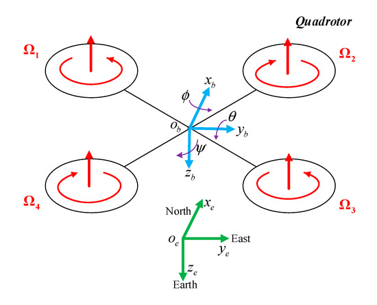
Figure 1.
Schematic view of the quadrotor unmanned aerial vehicles (QUAV).
According to Newton’s second law and the Euler moment of momentum equation, referring to [5,22,36,37], the complete dynamic model of a quadrotor is represented as follows
where is the mass of the quadrotor, is the acceleration of gravity, are the moments of inertia of the quadrotor, are the air resistance coefficients, is the unmodeled dynamics or external interference, where at least include the neglected gyro effect, respectively, and the terms contain gust disturbance. The terms denote the total thrust and three torques produced by the four rotors, respectively, and are expressed as
where is the length between the center of the aircraft and the rotor, are constants, called the lift coefficient and inverse torque coefficient, respectively, which can be determined experimentally, and are the angular velocities of the propellers.
3. HODFC Scheme for QUAV
3.1. Quadrotor Control Structure with Semi-Autopilot
For a quadrotor, it is generally necessary to design a controller to directly control the rotation speed of the propeller , and to generate a thrust and three moments to realize the position and attitude control. However, it is difficult for most researchers to build an autopilot from the underlying motor control. At present, many teams and companies have developed open-source semi-autopilots, such as Pixhawk and DJI. Therefore, research based on the existing semi-autopilot shall be conducted. One aspect of this work is to verify the new control theory; another aspect is the requirement to avoid the difficulty of directly modifying the underlying source code of the flight controller. The control structure of the quadrotor with a semi-autopilot is shown in Figure 2. The control command can directly control the following variables of the quadrotor: vertical speed , yaw angular velocity , horizontal velocity and , respectively. These variables further control the position and yaw angle of the quadrotor. Each channel from the control command to the variables , respectively, is stable because the semi-autopilot’s controller has dampers designed for these channels, making the quadrotor easy to control. However, each channel from the variable to the position and yaw angle , respectively, of the quadrotor is open-loop, so an additional position controller must be designed to complete the following tasks: for a given expected trajectory and expected yaw angle , make the system satisfy and .
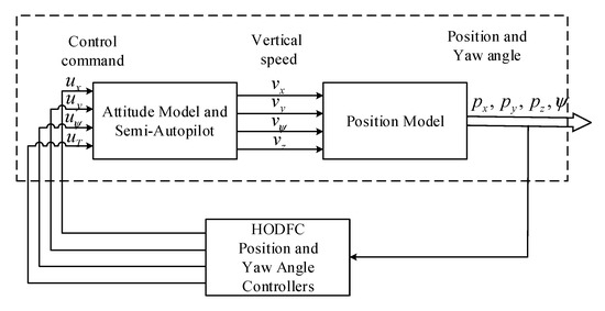
Figure 2.
Closed-loop block diagram of position control based on semi-autopilot.
3.2. HOD Design
The HOD and HODFC are designed based on time-varying single input single output (SISO) affine nonlinear systems with unknown models [23,24,38]. For the development of the HODFC controller of the quadrotor, its dynamic model must be expressed in an affine form. According to Equation (1), the quadrotor system can be divided into height, yaw and horizontal position channels, whose kinetics are expressed as:
where , and . The term represents the total disturbance, including the coupling term, external disturbances, the known model and unknown uncertainties corresponding to each channel. From another aspect, is the dynamic characteristics of the system, which may be time-varying or nonlinear. In the design process of HODFC, there is no need to know any information about , but indirectly has compensation through a filter module. For example, for the height channel of Equation (3), combining the third formula in Equation (1), , is also regarded as part of the total disturbance to ensure the correctness of Equation (3). The simplified processing of the model described here is to introduce the design process of the controller, while there is no information related to the model in the final control law.
The HOD is designed to observe the states of the system. The HOD can take any order , where is the order of the controlled quadrotor system. The measured output signal often contains some noise, so we need a filtering process before extracting its derivative. Essentially, the order of HOD also represents the number of integrators used in the design process. The greater the number of integrators, the smoother the derivatives extracted. For instance, if we need to extract the second-order derivative, at least a third-order HOD is needed. If the input signal is the first-order differentiable, when it feeds to one integrator, the output becomes the second-order differentiable. Even if the measured signal contains some noise, it becomes sufficiently smooth after feeding to many integrators. In HODFC design, only the second-order derivatives are needed, but the 5th HOD was selected for smoother derivatives, that is, .
We take the height channel, Equation (3), as an example to introduce the design process of the HOD. The dynamic equation of the HOD can be expressed as
where is the feeding signal, and are the states of the constructed system . The HOD function obtains the tracking signal and then obtains as the estimates of the derivatives and , respectively. Figure 3 is the block diagram of the HOD. It can be seen that state is not the derivative of (i.e., ), and also is not the derivative of . The next step is to make the following observation equation
where denote the observations of , respectively. From Figure 3, when tracks the input signal , the best observation of is the derivative of , which locates at the point labeling . In the same way, taking point is located. Thus the HOD satisfies , that is a derivative form to ensure accuracy.
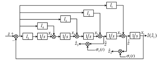
Figure 3.
The block diagram of fifth-order high order differentiator (HOD).
The parameters in the HOD are designed to make stable according to the root locus of the system [38].
There are too many parameters, , in the HOD, so we simplify it to have only one parameter. Taking the Laplace transform for both sides of Equation (6), the closed-loop transfer function from to is obtained as follows:
The open-loop transfer function is
Viewed from the structure of Figure 3 and considering the result of the open-loop transfer function, the HOD is a Type V servo system. If the input is a non-triangle signal, it can realize tracking without static error, and even if it is a sinusoidal signal, the high accuracy of estimation can be guaranteed. Equation (9) is the open-loop transfer function having four open-loop zeros. As long as the open-loop zeros of the closed-loop system are located in the left-half plane of the complex plane, poles of the closed-loop poles will also locate on the left-half plane when the gain is adjusted in a certain range. The gain can be found by locating the closed-loop poles on the negative real axis’s breakaway point. To keep stable and without loss of generality, let all zeros be the same negative real number ; in this way, the number of HOD parameters is reduced to 1. Then Equation (9) can be rewritten as
Once is selected properly, can be calculated; the root-locus method is used to obtain it. From Equation (8), the breakaway point of the root-locus can be calculated as , and it is chosen to be a pair of closed-loop poles on the negative real axis. According to the amplitude condition
where is the open-loop zero and is the open-loop zero and is the open-loop pole. Substituting into Equation (11), we obtain
Then from Equations (9), (10) and (12), we have
The symbol denotes the combination with . Usually, is chosen in the range of , depending on the accuracy requirement. Taking as an example, the root locus of the fifth-order HOD is shown in Figure 4. From Equation (10), system (HOD) has five root loci. The breakaway point is chosen as a pair of closed-loop poles, then . All the closed-loop poles are marked with “” in Figure 4; they are all located on the left-half plane. In fact, no matter how the gain changes, the three root loci marked as red, blue and green are always in the left-half plane. Since all the poles of the closed-loop HOD are located in the left-half plane, the HOD is stable.
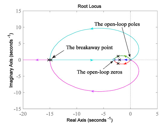
Figure 4.
Root loci of the fifth-order HOD ().
The parameter guarantees that HOD is an asymptotically stable system and satisfies convergence [23,24]. The parameter is independent of the system, which means that it can be tuned easily. To avoid the peaking pulse in the initial dynamic process, a restraint device [23,24] is added in Equation (7). The amended HOD observation equation is written as
where
where is called a restraint function and is set to be 100. Note that the restraint equation only takes effect in the initial time where , and after this moment . The block diagram representation of the amended HOD is demonstrated in Figure 3, where the are the HOD output and are also the observation values of . are the modified observation values for estimating . In the same way, we can design HOD to extract derivatives for a given reference input position .
Remark 1.
The HOD can extract the derivatives of a signal. The advantage of the HOD is as follows:
- (1)
- It has a filtering process because the number of integrators is more than the order of the extracted derivatives.
- (2)
- It has the derivative form, thereby having higher estimation accuracy.
- (3)
- It is simple, with only one parameter to adjust.
- (4)
- It is stable.
3.3. HODFC Design
As demonstrated in Figure 5, the HODFC scheme consists of three main parts, i.e., the HOD, the control gain , and the controller filter.
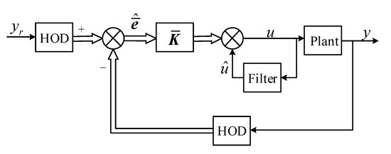
Figure 5.
The block diagram of the high-order differential feedback control (HODFC) scheme.
Denote the errors as , and , and denote the error vector , and the extended error vector . Combining Equation (3), the system error equation can be expressed as
where are the parameters in gain . Equation (16) can be converted to Equation (17)
where
If we want to keep the closed-loop system stable, should satisfy the Hurwitz matrix, and make , the polynomial be a Hurwitz polynomial. The pole arrangement structure is the most distinctive part of the HODFC. For instance, if the desired poles of the closed-loop system is , then the characteristic equation is , so . In the actual design process, the values of are calculated by selecting the appropriate poles. At the same time, the value can be reduced by an equivalent multiple to avoid excessive gain. For the stability of the closed-loop system, Equation (18) is necessary
then, we have
while are the terms relating to the system model and total perturbation, which cannot be determined exactly, and is unknown. However, from Equation (3), we have
thus contains both information and , but is underdetermined, so is replaced with , the estimate of . Although is underdetermined, the last instant was calculated. Because filter has a lag property, we design a filter as
thus, the problem of underdetermined control is solved.
Equation (21) is the controller filter, where is the filtering factor. The controller filter is globally uniformly stable and the value of approaches when , that is, . Then, from Equations (19)–(21), we get the control law of HODFC
and substituting Equations (3) and (22) into Equation (17), we have
from Equation (23), the unknown function and disturbance are indirectly counteracted by the filtering term for .
The term is a Hurwitz matrix and Equation (21), the closed-loop control system is asymptotically stable and satisfies
In practice, for the HODFC implementation, the error states used are obtained as estimates from the HOD. Then the final HODFC law based on HOD can be obtained, and there is no information related to the system model
Remark 2.
The HODFC of Equation (25) has the following advantages:
- (1)
- It does not rely on the system model and disturbance.
- (2)
- It makes the closed-loop system stable and behave in the desired assigned poles.
- (3)
- The control filter is designed to compensate for the unknown nonlinear model and disturbances.
From Figure 2, the control input are needed to design successively using Equation (25). Hence, in total, four HODFC controllers are needed to control the quadrotor system, and each HODFC contains two HODs. Although the controlled system is nonlinear and unknown, we use to replace through Equation (21), and the convergence is affirmed by . Therefore, the nonlinear and unknown problem is compensated or solved, and the total closed-loop system operates linearly with the desired poles. In practice, the filtering factor is not necessarily large but is within the scope accordingly.
4. Experimental Results
To verify the effectiveness of the HODFC, a physical experiment was carried out by using the indoor optical positioning system platform shown in Figure 6. The experimental setup consists of a miniature quadrotor, eight optical cameras, wireless routers and switches, and two personal computers as the ground control station. The quadrotor used for the experiment (shown in Figure 7) is a ZY-B/P type provided by Beijing Zhuoyi Intelligent Technology Co., Ltd. Four photosensitive balls attached to the fuselage reflect infrared light from the optical cameras and can be located by the positioning system. The quadrotor attitude and position data are transmitted back to the ground control station via wireless routers and switches to form an entirely closed-loop system.
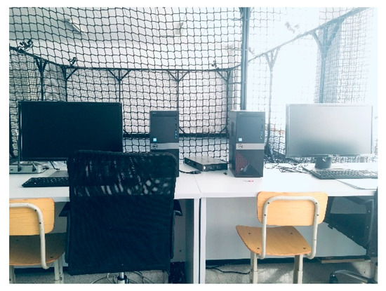
Figure 6.
The indoor optical positioning system platform.
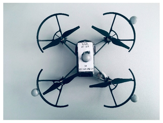
Figure 7.
Experimental ZY-B/P type quadrotor.
It should be noted that the flight mission is completed in the ground control station, including the design of the HODFC and the tuning of parameters. The quadrotor only has a tiny size, although we can roughly measure the mass of the quadrotor and the length between the center of the quadrotor and the rotor, the exact values of the moments of inertia, the air resistance coefficient, lift coefficient and inverse torque coefficient are unknown. The accurate mathematical model of the experimental quadrotor cannot be determined, therefore, a PID controller is selected for the comparison experiment. The sliding mode, back-step, or robust control are model-dependent. Although these methods are allowed to have uncertainty and disturbance under some assumptions, at least the normal part must be known, so they cannot be tested for this experiment and the unknown model. However, the PID and the HODFC can be used because they just need tuning of the parameters.
Three different sets of experiments are performed to show the control performance of HODFC on the static trajectory, dynamic trajectory and external disturbance. At the same time, the PID comparison experiments are performed. The HODFC and the PID parameters are selected carefully based on a trial and error method, to achieve the best control effect possible, which are listed in Table 1 and Table 2, respectively. Simultaneously, the idea of the pole assignment structure is also applied to the HODFC parameters determination process. For example, the pole of gain of the position is selected as , and height ; the value of can then be obtained by scaling the gain multiple. It is noted that the yaw and height are independent channels, and the second-order derivative information is removed to avoid noise interference caused by high-order derivative information. All the parameters remain unchanged during the experiment. Both the HODFC and the PID controllers are model-independent.

Table 1.
The values of parameters of the HODFC.
Table 2.
The values of parameters of the proportional-integral-derivative (PID).
To make the experiment results more convincing, the numerical performance metrics are presented. The obtained error signals are used as the difference between the reference trajectory and the actual trajectory, to calculate a numerical performance index. The error-based performance metrics are
where denotes the number of collected data, is the sampling frequency of the experimental device, is the time, and is the trajectory tracking error at time . MAE, IAE and ITAE stand for the mean absolute error, integral of absolute error and integral of time-weighted absolute error, respectively.
4.1. Static Trajectory Tracking
The effectiveness of both the HODFC scheme and the PID controller for a static trajectory in height and yaw channel are analyzed in this subsection. The reference trajectories of height and yaw are defined as and for . The tracking responses of the quadrotor tracking trajectory obtained using the two controllers are shown in Figure 8 and Figure 9. As can be seen from those two figures, overshoot occurs in the PID controller response, while the HODFC scheme not only well suppresses the occurrence of overshoot, it also has less settling time than that of the PID. A small fluctuation in the PID scheme occurs around 20 and 50 s without any external interference in the dashed box of Figure 9. The tracking errors and control output, i.e., are given in those figures as well. It can be seen that both control output values and errors stay within reasonable ranges. The numerical performance metrics are listed in Table 3. The HODFC scheme has a smaller performance metric compared with the PID. The improvement ratio between the PID and the HODFC more intuitively show the difference between the performance of the two control strategies. The bigger the ratio, the better the control effect of the HODFC relative to the PID.
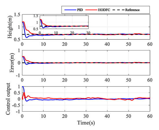
Figure 8.
Experimental results with a fixed height of 0.7 m.
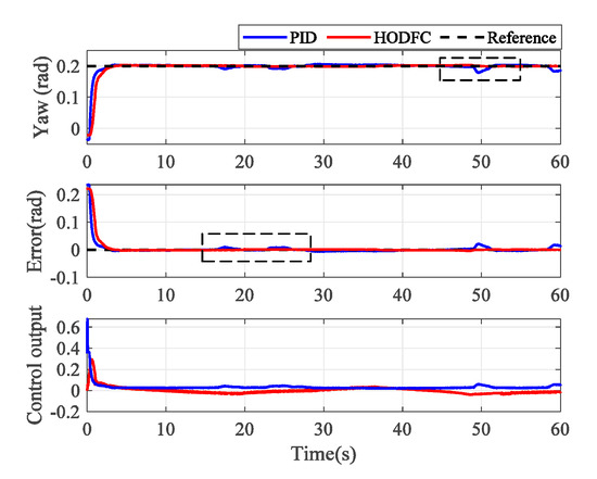
Figure 9.
Experimental results with a fixed yaw angle of 0.2 rad.
Table 3.
Numerical performance metrics of the static trajectory.
4.2. Dynamic Trajectory Tracking
The maneuver flight experiments are carried out in this subsection. The reference trajectories of height and yaw are defined as and for . The results of the dynamic tracking trajectory are shown in Figure 10 and Figure 11. The height and yaw can be achieved by both methods, and the tracking errors are driven into a small region around zero by the HODFC scheme. However, the tracking errors with PID control in the dynamic process performs poorly as there is always a large delay between the actual trajectory of the quadrotor and the reference trajectory. It can also be seen from the control output that the PID control output lags behind the HODFC control output, which results from the condition that the quadrotor is not sensitive enough to the change of trajectory.
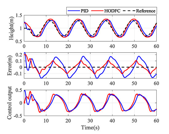
Figure 10.
Experimental results of height with a sinusoidal function reference.
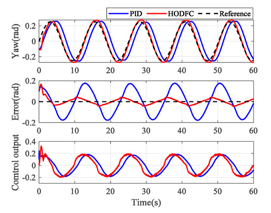
Figure 11.
Experimental results of yaw with a sinusoidal function reference.
For the spatial plane trajectory tracking, the quadrotor tracks a circle in the x-y plane, the radius of the tracked circle is set as , and the reference trajectory equation is expressed as for . The obtained results are illustrated in Figure 12 where the black circle denotes the reference track. Compared with the blue trajectory controlled by the PID, the red trajectory controlled by the HODFC is closer to the reference trajectory, and there is no overshoot in the direction in the initial dynamic process. The 3D trajectory tracking is shown in Figure 13. To show the spatial plane trajectory in more detail, the position, error and control output of the and directions are given in Figure 14 and Figure 15, respectively. Obviously, there is always much more error between the blue curve obtained by PID control and the black reference curve, which means that the PID control cannot achieve a good performance in maneuvering flights. The large error in the PID control is still caused by the lag of the control output. In comparison, the red curve executed by the HODFC can track the trajectory with a smaller error. The control output is also kept within a reasonable range, which means less damage to the actuator. In dynamic tracking experiments, the HODFC can react faster to trajectory changes, thereby exhibiting higher control accuracy. The performance of the HODFC is significantly improved over that of the PID. The numerical performance metrics in Table 4 also show that the HODFC scheme has excellent performance with the improvement ratios of around 2 to 5 with respect to the PID method.
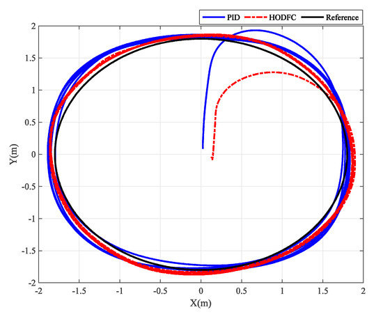
Figure 12.
Experimental results of the spatial plane trajectory tracking.
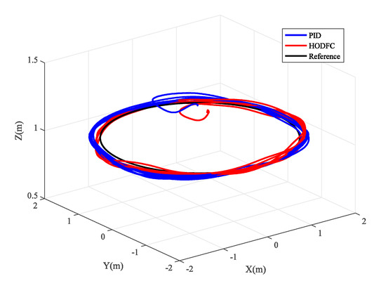
Figure 13.
Experimental results of 3D trajectory tracking.
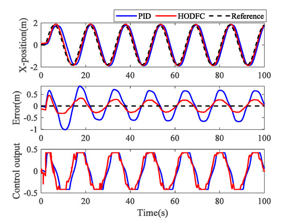
Figure 14.
Experimental results of space spatial trajectory tracking in the x position.
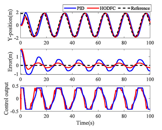
Figure 15.
Experimental results of space spatial trajectory tracking in the y position.
Table 4.
Numerical performance metrics of the dynamic trajectory.
4.3. Experiments with Disturbance
The ability of interference suppression is an essential indicator of a controller. In this case, the primary purpose is to prove the interference suppression performance of the HODFC on a quadrotor. After the quadrotor has stabilized for a while, we touched the quadrotor’s fuselage with a pen to change its height or attitude. The results of the experiment with human disturbance are provided in Figure 16 and Figure 17. From these figures, the HODFC method quickly drives the quadrotor to the preset height or angle after the disturbance occurs, and the steady-state error is close to zero. The output value of the controller is also adjusted to prevent external interference. During quadrotor flight, its attitude is susceptible to gusts. Therefore, we designed additional wind disturbance experiments for the yaw channel. After the yaw angle has stabilized, a small electric fan is used to blow the quadrotor with the same wind speed and angle. Figure 18 shows the experimental trajectory tracking results, errors and control output. Table 5 shows the calculated numerical results. The improvement ratios of the HODFC to the PID are around 1.8–3.4. As the gusts continued, the quadrotor angle with the HODFC trembled sharply, but remained near the set value. When the gusts disappear, the state of the quadrotor quickly stabilizes with little error. In contrast, for the PID controller, the fuselage has a huge shake when gusts occur and disappear, which means that the PID control is very sensitive to external interference and has low interference suppression, and there is a small steady-state error in the final state. Therefore, we can conclude that HODFC has a strong ability to resist external interference.
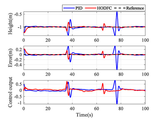
Figure 16.
Experimental results of height with human interference.
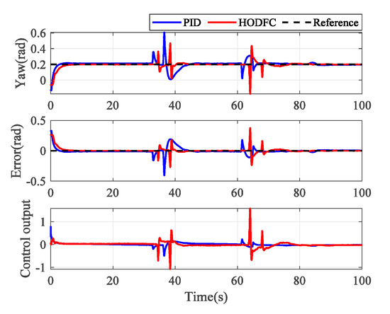
Figure 17.
Experimental results of yaw with human interference.
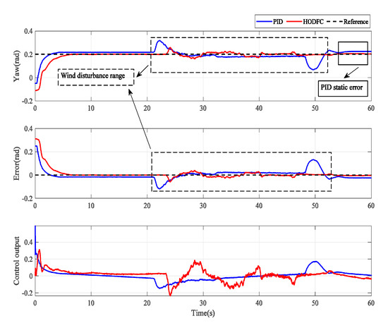
Figure 18.
Experimental results of yaw with wind disturbance.
Table 5.
Numerical performance metrics of static trajectory with disturbance.
5. Conclusions
In this paper, the quadrotor model was analyzed to fit the form of the affine nonlinear system used for the HODFC. The HODFC scheme based on the fifth HOD was applied to the quadrotor, which acts as a position controller in the semi-autopilot experimental platform. The HOD can extract the derivatives of the reference input and outputs of the system with high precision. The stability of the HOD was proved, and only one meaningful parameter is needed to choose. The stability of the HODFC designed for the quadrotor UAV was proved, and parameters can be easily selected according to the requirement. The HODFC does not need to use the model or disturbance information to control the system. To analyze the trajectory tracking performance of the HODFC scheme, three different sets of experiments were carried out on the static trajectory tracking, dynamic trajectory tracking and static trajectory tracking with disturbance. The parameters were tuned and carefully designed for comparison with the PID controller. The experimental results were analyzed from both visual and data aspects, which support the superiority of the HODFC scheme over the traditional PID controller. Our future work will improve the HODFC strategy, compare it with additional control strategies, and apply it to additional practical engineering systems.
Author Contributions
Conceptualization, G.Q.; data curation, X.G., X.L. and J.G.; project administration, S.M.; software, X.L.; data interpretation, S.M.; writing—original draft preparation, S.M.; writing—review and editing, G.Q. All authors have read and agreed to the published version of the manuscript.
Funding
This work was supported by the National Natural Science Foundation of China (61873186), the Key Projects of Tianjin National Science Foundation (18JCZDJC96700) and the Scientific Research Project of Tianjin Education Commission (2019KJ013).
Conflicts of Interest
The authors declare no conflict of interest.
References
- Qi, G.; Huang, D. Modeling and dynamical analysis of a small-scale unmanned helicopter. Nonlinear Dyn. 2019, 98, 2131–2145. [Google Scholar] [CrossRef]
- Hood, S.; Benson, K.; Hamod, P.; Madison, D.; O’Kane, J.M.; Rekleitis, I. Bird’s eye view cooperative exploration by UGV and UAV. In Proceedings of the International Conference on Unmanned Aircraft Systems, Miami, FL, USA, 13–16 June 2017; pp. 247–255. [Google Scholar]
- Yuan, C.; Liu, Z.; Zhang, Y. Aerial images-based forest fire detection for firefighting using optical remote sensing techniques and unmanned aerial vehicles. J. Intell. Robot. Syst. 2017, 88, 1–20. [Google Scholar] [CrossRef]
- Pierson, A.; Ataei, A.; Paschalidis, I.; Schwager, M. Cooperative multi-quadrotor pursuit of an evader in an environment with no-fly zones. In Proceedings of the IEEE International Conference on Robotics and Automation, Stockholm, Sweden, 16–21 May 2016; pp. 320–326. [Google Scholar]
- Bi, H.; Qi, G.; Hu, J. Modeling and analysis of chaos and bifurcations for the attitude system of a quadrotor unmanned aerial vehicle. Complexity 2019, 2019, 6313925-1-16. [Google Scholar] [CrossRef]
- Li, Y.; Song, S. A survey of control algorithms for quadrotor unmanned helicopter. In Proceedings of the IEEE International Conference on Advanced Computational Intelligence, Nanjing, China, 18–20 October 2012; pp. 365–369. [Google Scholar]
- Mu, B.; Zhang, K.; Shi, Y. Integral sliding mode flight controller design for a quadrotor and the application in a heterogeneous multi-agent system. IEEE Trans. Ind. Electron. 2017, 64, 9389–9398. [Google Scholar] [CrossRef]
- Tian, B.; Liu, L.; Lu, H.; Zuo, Z.; Zong, Q.; Zhang, Y. Multivariable finite time attitude control for quadrotor UAV: Theory and experimentation. IEEE Trans. Ind. Electron. 2017, 65, 2567–2577. [Google Scholar] [CrossRef]
- Liu, H.; Wang, X.; Zhong, Y. Quaternion-based robust attitude control for uncertain robotic quadrotors. IEEE Trans. Ind. Inform. 2015, 11, 406–415. [Google Scholar] [CrossRef]
- Salih, A.; Moghavvemi, M.; Mohamed, H.; Gaeid, K.S. Flight PID controller design for a UAV quadrotor. Sci. Res. Essays 2010, 5, 3660–3667. [Google Scholar]
- Vázquez, S.; Valenzuela, J. A new nonlinear PI/PID controller for quadrotor posture regulation. In Proceedings of the IEEE Electronics, Robotics and Automotive Mechanics Conference, Morelos, Mexico, 28 September–1 October 2010; pp. 642–647. [Google Scholar]
- Gao, Y.; Chen, D.; Li, R. Research on control algorithm of microquadrotor aircraft. Comput. Mod. 2011, 194, 4–7. [Google Scholar]
- Sangyam, T.; Laohapiengsak, P.; Chongcharoen, W.; Nilkhamhang, I. Path tracking of UAV using self-tuning PID controller based on fuzzy logic. In Proceedings of the Society of Instrument and Control Engineers Conference, Taipei, Taiwan, 18–21 August 2010; pp. 1265–1269. [Google Scholar]
- Efe, M. Neural network assisted computationally simple PIλDμ control of a quadrotor UAV. IEEE Trans. Ind. Inform. 2011, 7, 354–361. [Google Scholar] [CrossRef]
- Han, J. From PID to active disturbance rejection control. IEEE Trans. Ind. Electron. 2009, 56, 900–906. [Google Scholar] [CrossRef]
- Gao, Z. Scaling and bandwidth-parameterization based controller tuning. In Proceedings of the American Control Conference, Minneapolis, MN, USA, 14–16 June 2006; pp. 4989–4996. [Google Scholar]
- Nie, Z.; Liu, R. Inverted pendulum angle control design and experimental studies under complex conditions. Inf. Control 2016, 45, 506–512. [Google Scholar]
- Sun, M.; Wang, Z.; Wang, Y.; Chen, Z. On low-velocity compensation of brushless dc servo in the absence of friction model. IEEE Trans. Ind. Electron. 2013, 60, 3897–3905. [Google Scholar] [CrossRef]
- Chen, Z.; Cheng, Y.; Sun, M.; Sun, Q. Surveys on theory and engineering applications for linear active disturbance rejection control. Inf. Control 2017, 46, 257–266. [Google Scholar]
- Zhao, Z.; Guo, B. On convergence of nonlinear active disturbance rejection control for SISO nonlinear systems. J. Dyn. Control Syst. 2016, 22, 385–412. [Google Scholar] [CrossRef]
- Yang, H.; Cheng, L.; Xia, Y.; Yuan, Y. Active disturbance rejection attitude control for a dual closed-loop quadrotor under gust wind. IEEE Trans. Control Syst. Technol. 2018, 26, 1400–1405. [Google Scholar] [CrossRef]
- Li, X.; Chen, Y. Reduced-order active disturbance rejection control for quadrotor aircraft. Electron. Opt. Control 2019, 26, 43–48, 72. [Google Scholar]
- Qi, G.; Chen, Z.; Yuan, Z. Model-free control of affine chaotic systems. Phys. Lett. A 2005, 344, 189–202. [Google Scholar] [CrossRef]
- Qi, G.; Chen, Z.; Yuan, Z. Adaptive high order differential feedback control for affine nonlinear system. Chaos Solitons Fractals 2008, 37, 308–315. [Google Scholar] [CrossRef]
- Xue, W.; Xue, Y.; Qi, G.; Gao, J.; Zheng, S. Study of high order differential feedback control of DC-link voltage in active power filter. In Proceedings of the IEEE International Conference on Automation and Logistics, Jinan, China, 18–21 August 2007; pp. 1063–1066. [Google Scholar]
- Du, S.; Wyk, B.; Qi, G.; Tu, C. Chaotic system synchronization with an unknown master model using a hybrid HOD active control approach. Chaos Solitons Fractals 2009, 42, 1900–1913. [Google Scholar] [CrossRef]
- Nyabundi, S.; Qi, G.; Hamam, Y.; Munda, J. DC motor control via high order differential feedback control. In Proceedings of the AFRICON, Nairobi, Kenya, 23–25 September 2009; pp. 1–5. [Google Scholar]
- Shi, X.; Dai, Y.; Liu, Z.; Qi, G. High order differentialfeedback controller and its application in servo control system of NC machine tools. In Proceedings of the IEEE International Conference on System Science, Yichang, China, 12–14 November 2010; pp. 241–244. [Google Scholar]
- Faradja, P.; Qi, G. Robustness based comparison between a sliding mode controller and a model free controller with the approach of synchronization of nonlinear systems. In Proceedings of the International Conference on Control, Automation and Systems, Busan, Korea, 13–16 October 2015; pp. 36–40. [Google Scholar]
- Agee, J.; Bingul, Z.; Kizir, S. Higher-order differential feedback control of a flexible-joint manipulator. J. Vib. Control 2015, 21, 1976–1986. [Google Scholar] [CrossRef]
- Agee, J.; Bingul, Z.; Kizir, S. Trajectory and vibration control of a single-link flexible joint manipulator using a distributed higher order differential feedback controller. J. Dyn. Syst. Meas. Control 2017, 139, 081006. [Google Scholar] [CrossRef]
- Ayas, M.; Sahin, E.; Altas, I. High order differential feedback controller design and implementation for a stewart platform. J. Vib. Control 2019, 26, 976–988. [Google Scholar] [CrossRef]
- Ayas, M. Design of an optimized fractional high-order differential feedback controller for an AVR system. Electr. Eng. 2019, 101, 1221–1233. [Google Scholar] [CrossRef]
- Yi, K.; Gu, F.; Yang, L.; He, Y.; Han, J. Sliding model control for a quadrotor slung load system. In Proceedings of the Chinese Control Conference, Dalian, China, 26–28 July 2017; pp. 3694–3703. [Google Scholar]
- Guo, Y.; Jiang, B.; Zhang, Y. A novel robust attitude control for quadrotor aircraft subject to actuator faults and wind gusts. IEEE/CAA J. Autom. Sin. 2018, 5, 292–300. [Google Scholar] [CrossRef]
- Zhao, B.; Xian, B.; Zhang, Y.; Zhang, X. Nonlinear robust adaptive tracking control of a quadrotor UAV via immersion and invariance methodology. IEEE Trans. Ind. Electron. 2015, 62, 2891–2902. [Google Scholar] [CrossRef]
- Zhang, Y.; Chen, Z.; Zhang, X.; Sun, Q.; Sun, M. A novel control scheme for quadrotor UAV based upon active disturbance rejection control. Aerosp. Sci. Technol. 2018, 79, 601–609. [Google Scholar] [CrossRef]
- Qi, G.; Chen, Z.; Xue, W.; Yuan, Z. A new differential state estimator and controller for nonlinear stochastic system. Chin. J. Electron. 2004, 32, 693–696. [Google Scholar]
Publisher’s Note: MDPI stays neutral with regard to jurisdictional claims in published maps and institutional affiliations. |
© 2020 by the authors. Licensee MDPI, Basel, Switzerland. This article is an open access article distributed under the terms and conditions of the Creative Commons Attribution (CC BY) license (http://creativecommons.org/licenses/by/4.0/).