Figure 1.
(a) The architecture of 2D squeeze-and-excite block. represents the channels of a computing unit , and the feature map size of each channel is ; (b) the computation of 1D squeeze-and-excite block used in this system.
Figure 1.
(a) The architecture of 2D squeeze-and-excite block. represents the channels of a computing unit , and the feature map size of each channel is ; (b) the computation of 1D squeeze-and-excite block used in this system.
Figure 2.
The structure of a basic LSTM cell, where , , , respectively represent the input gate, forget gate, output gate and memory state cell. The update of each gate and state can be found in Equations (2)–(7).
Figure 2.
The structure of a basic LSTM cell, where , , , respectively represent the input gate, forget gate, output gate and memory state cell. The update of each gate and state can be found in Equations (2)–(7).
Figure 3.
Illustration of attention mechanism. The input is a sequence with length and dimension , which is mapped to a one-dimensional score by the linear layer, and these scores are then passed through the Softmax function to give the set of weights.
Figure 3.
Illustration of attention mechanism. The input is a sequence with length and dimension , which is mapped to a one-dimensional score by the linear layer, and these scores are then passed through the Softmax function to give the set of weights.
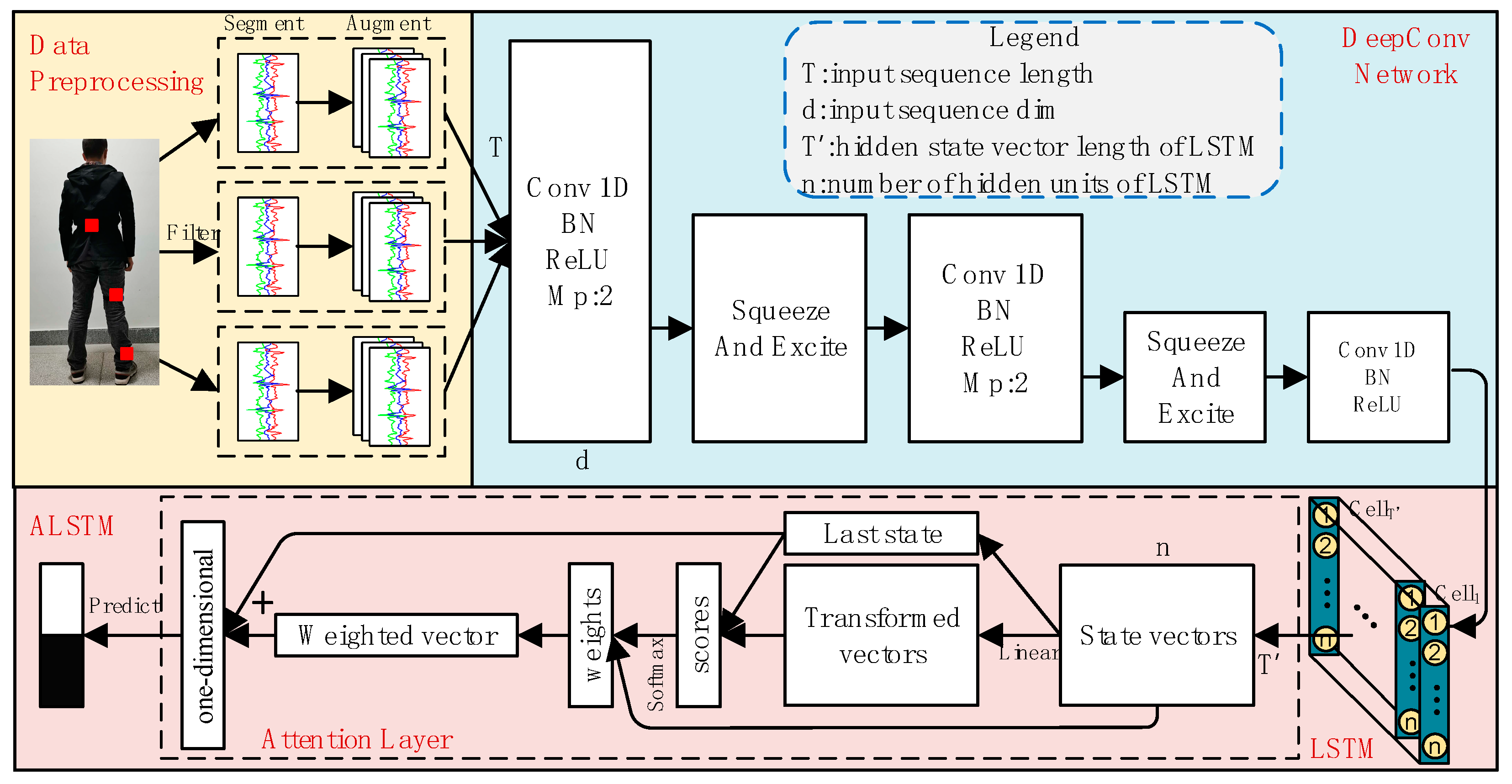
Figure 4.
The architecture of the proposed SEC-ALSTM. Conv 1D is a one-dimensional convolutional layer, LSTM is a long short-term memory recurrent neural network, squeeze-and-excitation block is used to converge the global information of each channel of the network. “Bn”, “ReLU” and “MP” are the abbreviations of “Batchnormalization”, “Rectified Linear Unit”, and “Max pooling layer” respectively. is the length of data instance in the temporal dimension, is the dimension, is the hidden state vector length of LSTM, and is the number of hidden units of LSTM.
Figure 5.
(b,d) are the signals in (a,c) after outlier processing, and (e–h) are the power spectra of the signal in (a–d).
Figure 5.
(b,d) are the signals in (a,c) after outlier processing, and (e–h) are the power spectra of the signal in (a–d).
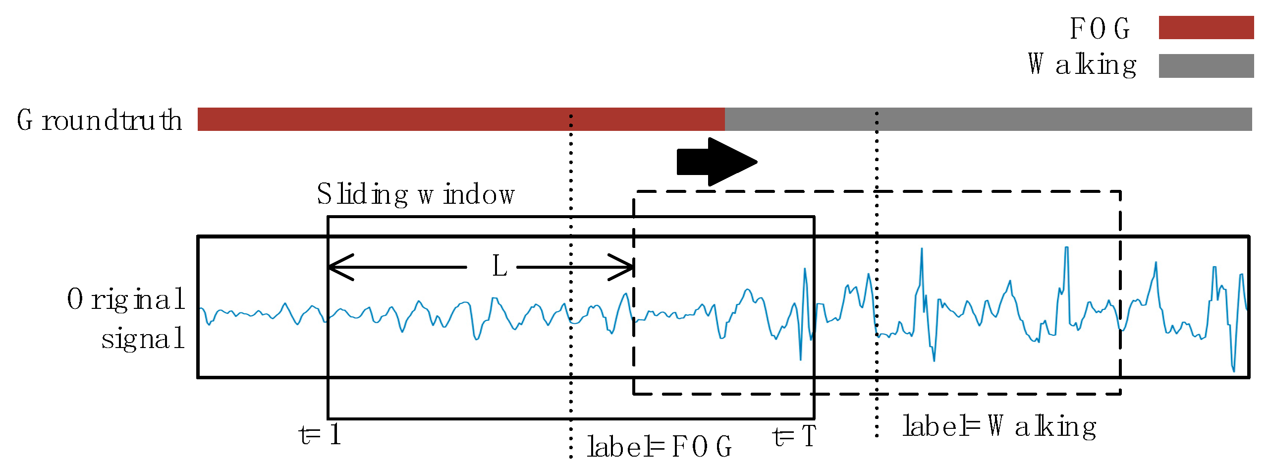
Figure 6.
Data segmentation and labeling. The original signals are segmented by a sliding window of length T. The step size of the window is L. The activity label within each sequence is considered to be the ground truth label with the most occurrences of that window.
Figure 6.
Data segmentation and labeling. The original signals are segmented by a sliding window of length T. The step size of the window is L. The activity label within each sequence is considered to be the ground truth label with the most occurrences of that window.
Figure 7.
(a–c) are the original three-axis acceleration signals of standing, walking and freezing of gait (FOG), (d–f) are the augmented signals.
Figure 7.
(a–c) are the original three-axis acceleration signals of standing, walking and freezing of gait (FOG), (d–f) are the augmented signals.
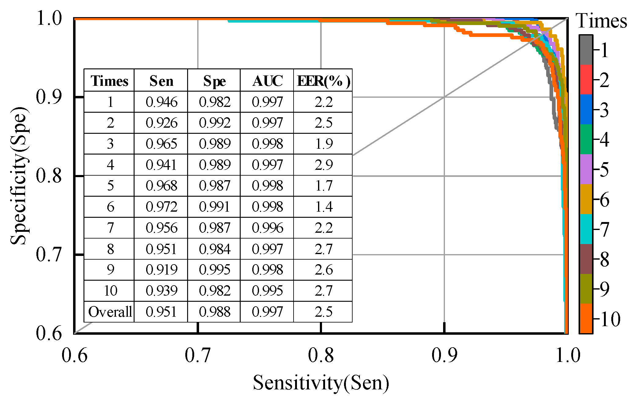
Figure 8.
Specificity vs. sensitivity curves, area under the curve (AUC), and equal error rate (EER) for the second patient-dependent experiment; the samples used for training and testing were from all patients.
Figure 8.
Specificity vs. sensitivity curves, area under the curve (AUC), and equal error rate (EER) for the second patient-dependent experiment; the samples used for training and testing were from all patients.
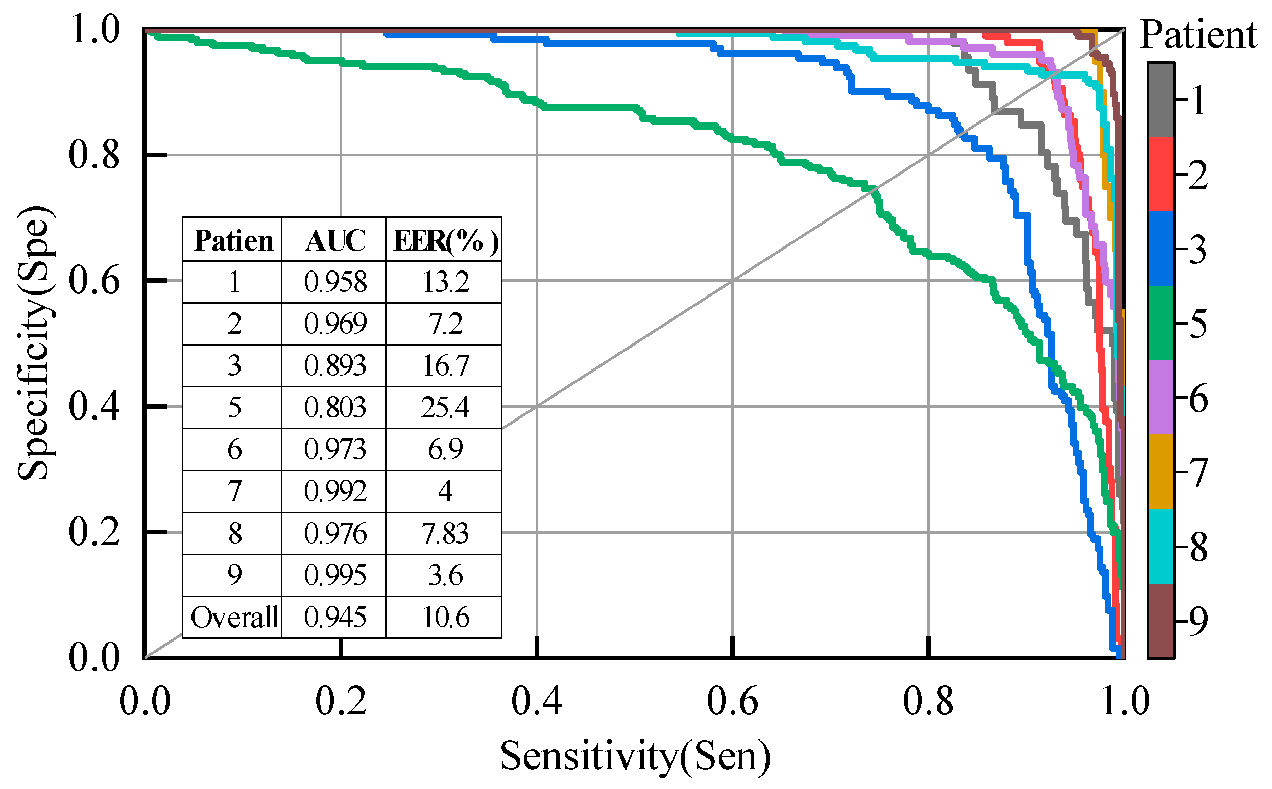
Figure 9.
Results of each patient for the proposed model using leave-one-subject-out (LOSO) evaluation, excluding patients #4 and #10.
Figure 9.
Results of each patient for the proposed model using leave-one-subject-out (LOSO) evaluation, excluding patients #4 and #10.
Figure 10.
Specificity vs. sensitivity curves, and AUC for different models with a LOSO evaluation.
Figure 10.
Specificity vs. sensitivity curves, and AUC for different models with a LOSO evaluation.
Figure 11.
Specificity vs. sensitivity curves, AUC and EER for different sensor placement and different sampling frequency with LOSO evaluation.
Figure 11.
Specificity vs. sensitivity curves, AUC and EER for different sensor placement and different sampling frequency with LOSO evaluation.
Table 1.
Parameters of the hardware platform.
Table 1.
Parameters of the hardware platform.
| Central Processing Unit | Graphics Processing Unit | Graphics Memory | Computer Memory |
|---|
| Intel(R) Core(TM) i5-9400 | Nvidia GeForce RTX 2060 | 6 GB | 8 GB |
Table 2.
The main attributes of the Daphnet dataset.
Table 2.
The main attributes of the Daphnet dataset.
| Number of Patients | Age (Years) | H & Y in ON | Sampling Rate (Hz) | Test Duration (Mins) | Number of Freeze Events |
|---|
| 10 (3 females) | 66.4 ± 4.8 | 2.6 ± 0.65 | 64 | 500 | 237 |
Table 3.
The class distribution of data instances for each patient. The data instance are obtained by segmenting the acceleration signals using a sliding window, where the length of the sliding window is 256 and the step size is 4.
Table 3.
The class distribution of data instances for each patient. The data instance are obtained by segmenting the acceleration signals using a sliding window, where the length of the sliding window is 256 and the step size is 4.
| Class | Patient |
|---|
| 1 | 2 | 3 | 4 | 5 | 6 | 7 | 8 | 9 | 10 | Overall |
|---|
| Walking | 16,110 | 11,310 | 8557 | 12,032 | 11,794 | 13,548 | 16,770 | 4915 | 9646 | 16,670 | 121,352 |
| FOG | 1434 | 2856 | 4241 | 0 | 7514 | 1907 | 1053 | 2896 | 4053 | 0 | 25,954 |
Table 4.
The hyper-parameters for the model proposed in this study.
Table 4.
The hyper-parameters for the model proposed in this study.
| Learning Parameter | Value or Method |
|---|
| Batch size | 64 |
| Regularization | BatchNormalization |
| Learning rate | 0.001 |
| Reduction ratio(r) | 8 |
| Number of Conv.Filters | 64 |
| Kernel size (k1) | 7 |
| Kernel size (k2) | 5 |
| Kernel size (k3) | 3 |
| Hidden Units (n) | 128 |
| Input Dimension (d) | 9 |
Table 5.
The results of a 10-fold cross-validation (R10Fold) evaluation. The samples used for training and testing were from the same patient. TP, TN, FP, and FN are abbreviations of true positive, true negative, false positive and false negative, respectively. Subject #4 and #10 did not have FOG during this study.
| Patient | TP | TN | FP | FN | Sensitivity | Specificity | Accuracy | F1-Score |
|---|
| 1 | 1424 | 16,097 | 13 | 10 | 0.993 | 0.999 | 0.999 | 0.992 |
| 2 | 2834 | 11,281 | 22 | 29 | 0.992 | 0.997 | 0.996 | 0.991 |
| 3 | 4198 | 8516 | 43 | 41 | 0.990 | 0.995 | 0.994 | 0.990 |
| 4 | 12,032 | 0 | 0 | 0 | - | 1.000 | 1.000 | - |
| 5 | 7406 | 11,728 | 66 | 108 | 0.986 | 0.994 | 0.991 | 0.988 |
| 6 | 1905 | 13,540 | 8 | 2 | 0.999 | 0.999 | 0.999 | 0.997 |
| 7 | 1032 | 16,757 | 13 | 21 | 0.980 | 0.999 | 0.998 | 0.984 |
| 8 | 2883 | 4950 | 10 | 13 | 0.996 | 0.998 | 0.997 | 0.996 |
| 9 | 4033 | 9610 | 36 | 20 | 0.995 | 0.996 | 0.996 | 0.993 |
| 10 | 16,670 | 0 | 0 | 0 | - | 1.000 | 1.000 | - |
| Overall | 25,710 | 121,141 | 211 | 244 | 0.991 | 0.998 | 0.997 | 0.991 |
Table 6.
The performance comparison of different approaches on the same dataset using a R10Fold evaluation.
Table 6.
The performance comparison of different approaches on the same dataset using a R10Fold evaluation.
| Reference | Description | Sensitivity | Specificity |
|---|
| Bachlin et al. [25] | FI index, energy in the frequency band 0.5–8 Hz | 0.781 | 0.869 |
| San-Segundo et al. [38] (reproducing Mazilu et al.’s system [46]) | Signal mean, standard deviation, variance, frequency entropy, energy, FI index, etc. | 0.934 | 0.939 |
| The proposed | DL-based feature learning | 0.951 | 0.988 |
Table 7.
The performance comparison of different approaches on the same dataset using a LOSO evaluation.
Table 7.
The performance comparison of different approaches on the same dataset using a LOSO evaluation.
| Reference | AUC | EER (%) |
|---|
| Mazilu et al. [46] (reproduced by San-Segundo et al.) | 0.900 | 17.3 |
| San-Segundo et al. [38] (deep neural network with 3 previous and 3 posterior windows) | 0.931 | 12.5 |
| The proposed | 0.945 | 10.6 |
Table 8.
The performance comparison of different neural network models on the same dataset using a LOSO evaluation.
Table 8.
The performance comparison of different neural network models on the same dataset using a LOSO evaluation.
| Reference | Description | Accuracy |
|---|
| Xia Yi et al. [37] | Deep convolutional neural networks with five-layer CNN | 0.807 |
| Ashour et al. [52] | Long Short Term Memory (LSTM) network based DL model | 0.834 |
| The proposed | Improved DL neural networks model | 0.919 |
Table 9.
Evaluation results of the effects of data augmentation, SE block, and attention mechanisms on model performance.
Table 9.
Evaluation results of the effects of data augmentation, SE block, and attention mechanisms on model performance.
| Model | Sensitivity | Specificity | AUC | EER (%) |
|---|
| SEC-ALSTM | 0.927 | 0.952 | 0.976 | 7.8 |
| SEC-ALSTM without DA | 0.875 | 0.923 | 0.949 | 10.4 |
| CALSTM | 0.914 | 0.879 | 0.956 | 9.2 |
| SEC-LSTM | 0.895 | 0.949 | 0.963 | 8.7 |
Table 10.
The detection performance for different sensor placement and different sampling frequency, using a LOSO evaluation.
Table 10.
The detection performance for different sensor placement and different sampling frequency, using a LOSO evaluation.
| Model | Sensitivity | Specificity | AUC | EER (%) |
|---|
| All three accelerometers + 64 Hz | 0.927 | 0.952 | 0.976 | 7.8 |
| Ankle accelerometer+ 64 Hz | 0.921 | 0.941 | 0.971 | 6.3 |
| Knee accelerometer+ 64 Hz | 0.901 | 0.905 | 0.953 | 9.7 |
| Back accelerometer+ 64 Hz | 0.829 | 0.908 | 0.932 | 11.8 |
| All three accelerometers + 48 Hz | 0.908 | 0.959 | 0.981 | 7.8 |
| All three accelerometers + 32 Hz | 0.908 | 0.967 | 0.983 | 7.8 |
| All three accelerometers + 16 Hz | 0.848 | 0.945 | 0.971 | 9.0 |
| All three accelerometers + 8 Hz | 0.816 | 0.912 | 0.927 | 13.0 |

 ,
, 


